Category Archives: r-index

A Meta-Scientific Perspective on “Thinking: Fast and Slow

2011 was an important year in the history of psychology, especially social psychology. First, it became apparent that one social psychologist had faked results for dozens of publications (https://en.wikipedia.org/wiki/Diederik_Stapel). Second, a highly respected journal published an article with the incredible claim that humans can foresee random events in the future, if they are presented without awareness (https://replicationindex.com/2018/01/05/bem-retraction/). Third, Nobel Laureate Daniel Kahneman published a popular book that reviewed his own work, but also many findings from social psychology (https://en.wikipedia.org/wiki/Thinking,_Fast_and_Slow).

It is likely that Kahneman’s book, or at least some of his chapters, would be very different from the actual book, if it had been written just a few years later. However, in 2011 most psychologists believed that most published results in their journals can be trusted. This changed when Bem (2011) was able to provide seemingly credible scientific evidence for paranormal phenomena nobody was willing to believe. It became apparent that even articles with several significant statistical results could not be trusted.

Kahneman also started to wonder whether some of the results that he used in his book were real. A major concern was that implicit priming results might not be replicable. Implicit priming assumes that stimuli that are presented outside of awareness can still influence behavior (e.g., you may have heard the fake story that a movie theater owner flashed a picture of a Coke bottle on the screen and that everybody rushed to the concession stand to buy a Coke without knowing why they suddenly wanted one). In 2012, Kahneman wrote a letter to the leading researcher of implicit priming studies, expressing his doubts about priming results, that attracted a lot of attention (Young, 2012).

Several years later, it has become clear that the implicit priming literature is not trustworthy and that many of the claims in Kahneman’s Chapter 4 are not based on solid empirical foundations (Schimmack, Heene, & Kesavan, 2017). Kahneman acknowledged this in a comment on our work (Kahneman, 2017).

We initially planned to present our findings for all chapters in more detail, but we got busy with other things. However, once in a while I am getting inquires about the other chapters (Engber). So, I am using some free time over the holidays to give a brief overview of the results for all chapters.

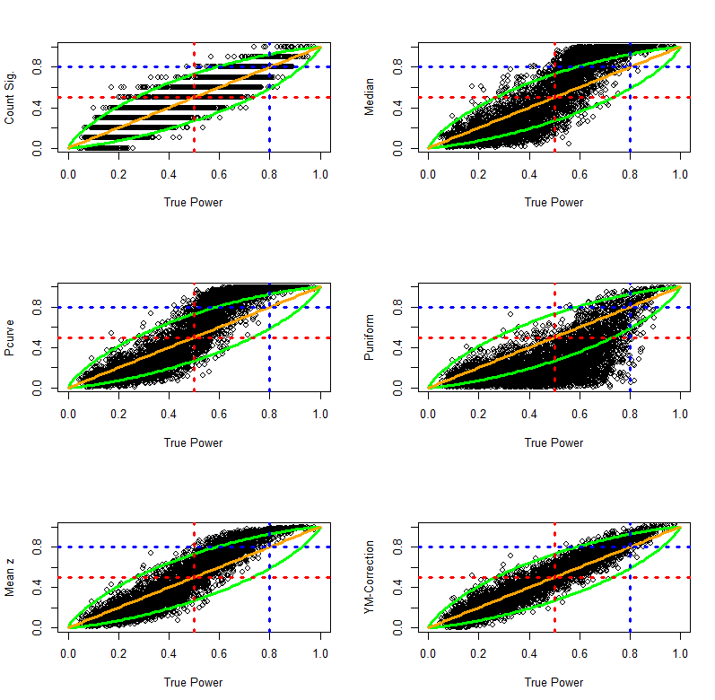
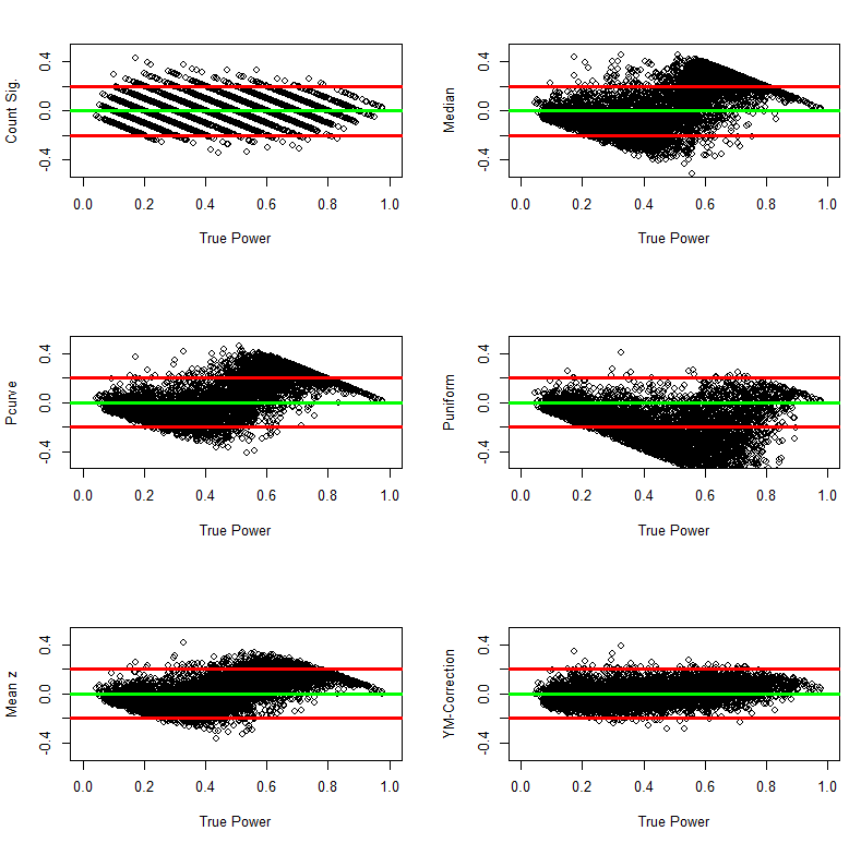
The Replicability Index (R-Index) is based on two statistics (Schimmack, 2016). One statistic is simply the percentage of significant results. In a popular book that discusses discoveries, this value is essentially 100%. The problem with selecting significant results from a broader literature is that significance alone, p < .05, does not provide sufficient information about true versus false discoveries. It also does not tell us how replicable a result is. Information about replicability can be obtained by converting the exact p-value into an estimate of statistical power. For example, p = .05 implies 50% power and p = .005 implies 80% power with alpha = .05. This is a simple mathematical transformation. As power determines the probability of a significant result, it also predicts the probability of a successful replication. A study with p = .005 is more likely to replicate than a study with p = .05.

There are two problems with point-estimates of power. One problem is that p-values are highly variable, which also produces high variability / uncertainty in power estimates. With a single p-value, the actual power could range pretty much from the minimum of .05 to the maximum of 1 for most power estimates. This problem is reduced in a meta-analysis of p-values. As more values become available, the average power estimate is closer to the actual average power.

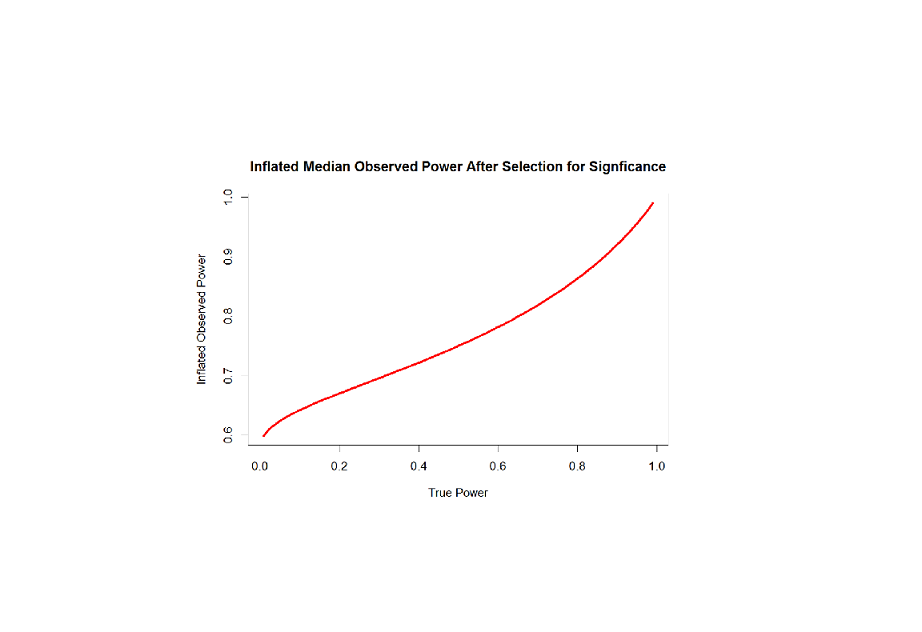
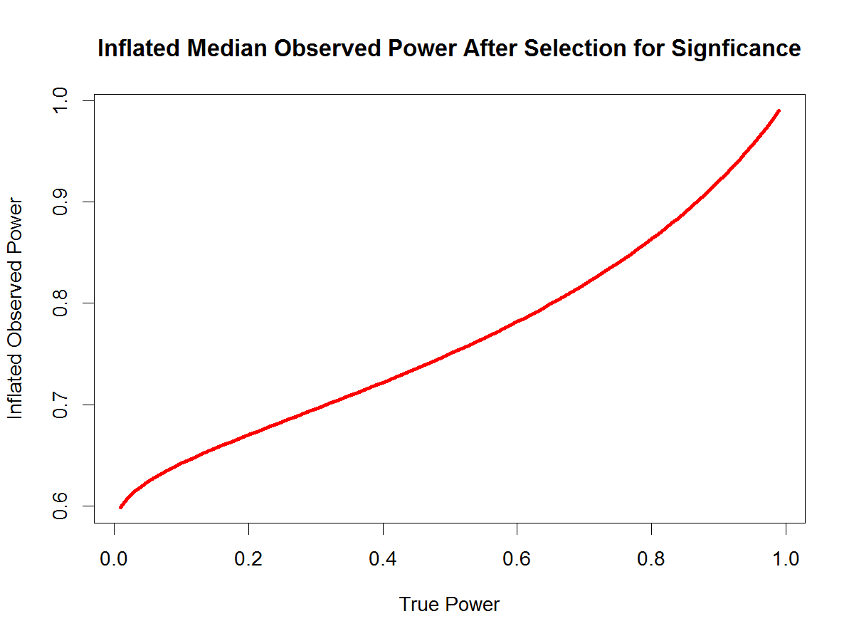
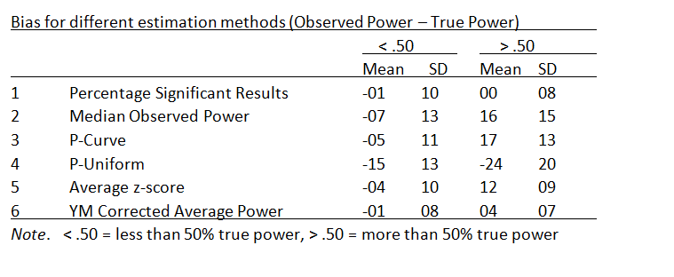
The second problem is that selection of significant results (e.g., to write a book about discoveries) inflates power estimates. This problem can be addressed by comparing the success rate or discovery rate (i.e., the percentage of significant results) with the average power. Without publication bias, the discovery rate should match average power (Brunner & Schimmack, 2020). When publication bias is present, the discovery rate exceeds average power (Schimmack, 2012). Thus, the difference between the discovery rate (in this case 100%) and the average power estimates provides information about the extend of publication bias. The R-Index is a simple correction for the inflation that is introduced by selecting significant results. To correct for inflation the difference between the discovery rate and the average power estimate is subtracted from the mean power estimate. For example, if all studies are significant and the mean power estimate is 80%, the discrepancy is 20%, and the R-Index is 60%. If all studies are significant and the mean power estimate is only 60%, the R-Index is 20%.

When I first developed the R-Index, I assumed that it would be better to use the median (e.g.., power estimates of .50, .80, .90 would produce a median value of .80 and an R-Index of 60. However, the long-run success rate is determined by the mean. For example, .50, .80, .90 would produce a mean of .73, and an R-Index of 47. However, the median overestimates success rates in this scenario and it is more appropriate to use the mean. As a result, the R-Index results presented here differ somewhat from those shared publically in an article by Engber.

Table 1 shows the number of results that were available and the R-Index for chapters that mentioned empirical results. The chapters vary dramatically in terms of the number of studies that are presented (Table 1). The number of results ranges from 2 for chapters 14 and 16 to 55 for Chapter 5. For small sets of studies, the R-Index may not be very reliable, but it is all we have unless we do a careful analysis of each effect and replication studies.

Chapter 4 is the priming chapter that we carefully analyzed (Schimmack, Heene, & Kesavan, 2017).Table 1 shows that Chapter 4 is the worst chapter with an R-Index of 19. An R-Index below 50 implies that there is a less than 50% chance that a result will replicate. Tversky and Kahneman (1971) themselves warned against studies that provide so little evidence for a hypothesis. A 50% probability of answering multiple choice questions correctly is also used to fail students. So, we decided to give chapters with an R-Index below 50 a failing grade. Other chapters with failing grades are Chapter 3, 6, 711, 14, 16. Chapter 24 has the highest highest score (80, wich is an A- in the Canadian grading scheme), but there are only 8 results.

Chapter 24 is called “The Engine of Capitalism”

A main theme of this chapter is that optimism is a blessing and that individuals who are more optimistic are fortunate. It also makes the claim that optimism is “largely inherited” (typical estimates of heritability are about 40-50%), and that optimism contributes to higher well-being (a claim that has been controversial since it has been made, Taylor & Brown, 1988; Block & Colvin, 1994). Most of the research is based on self-ratings, which may inflate positive correlations between measures of optimism and well-being (cf. Schimmack & Kim, 2020). Of course, depressed individuals have lower well-being and tend to be pessimistic, but whether optimism is really preferable over realism remains an open question. Many other claims about optimists are made without citing actual studies.

Even some of the studies with a high R-Index seem questionable with the hindsight of 2020. For example, Fox et al.’s (2009) study of attentional biases and variation in the serotonin transporter gene is questionable because single-genetic variant research is largely considered unreliable today. Moreover, attentional-bias paradigms also have low reliability. Taken together, this implies that correlations between genetic markers and attentional bias measures are dramatically inflated by chance and unlikely to replicate.

Another problem with narrative reviews of single studies is that effect sizes are often omitted. For example, Puri and Robinson’s finding that optimism (estimates of how long you are going to live) and economic risk-taking are correlated is based on a large sample. This makes it possible to infer that there is a relationship with high confidence. A large sample also allows fairly precise estimates of the size of the relationship, which is a correlation of r = .09. A simple way to understand what this correlation means is to think about the increase in predicting in risk taking. Without any predictor, we have a 50% chance for somebody to be above or below the average (median) in risk-taking. With a predictor that is correlated r = .09, our ability to predict risk taking increases from 50% to 55%.

Even more problematic, the next article that is cited for a different claim shows a correlation of r = -.04 between a measure of over-confidence and risk-taking (Busenitz & Barney, 1997). In this study with a small sample (N = 124 entrepreneurs, N = 95 managers), over-confidence was a predictor of being an entrepreneur, z = 2.89, R-Index = .64.

The study by Cassar and Craig (2009) provides strong evidence for hindsight bias, R-Index = 1. Entrepreneurs who were unable to turn a start-up into an operating business underestimated how optimistic they were about their venture (actual: 80%, retrospective: 60%).

Sometimes claims are only loosely related to a cited article (Hmieleski & Baron, 2009). The statement “this reasoning leads to a hypothesis: the people who have the greatest influence on the lives of others are likely to be optimistic and overconfident, and to take more risks than they realize” is linked to a study that used optimism to predict revenue growth and employment growth. Optimism was a negative predictor, although the main claim was that the effect of optimism also depends on experience and dynamism.

A very robust effect was used for the claim that most people see themselves as above average on positive traits (e.g., overestimate their intelligence) (Williams & Gilovich, 2008), R-Index = 1. However, the meaning of this finding is still controversial. For example, the above average effect disappears when individuals are asked to rate themselves and familiar others (e.g., friends). In this case, ratings of others are more favorable than ratings of self (Kim et al., 2019).

Kahneman then does mention the alternative explanation for better-than-average effects (Windschitl et al., 2008). Namely rather than actually thinking that they are better than average, respondents simply respond positively to questions about qualities that they think they have without considering others or the average person. For example, most drivers have not had a major accident and that may be sufficient to say that they are a good driver. They then also rate themselves as better than the average driver without considering that most other drivers also did not have a major accident. R-Index = .92.

So, are most people really overconfident and does optimism really have benefits and increase happiness? We don’t really know, even 10 years after Kahneman wrote his book.

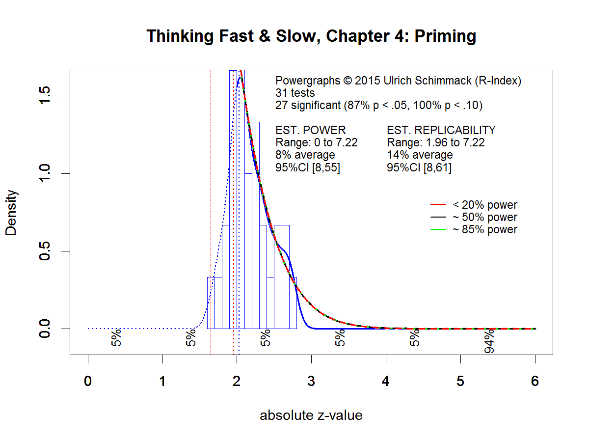
Meanwhile, the statistical analysis of published results has also made some progress. I analyzed all test statistics with the latest version of z-curve (Bartos & Schimmack, 2020). All test-statistics are converted into absolute z-scores that reflect the strength of evidence against the null-hypothesis that there is no effect.

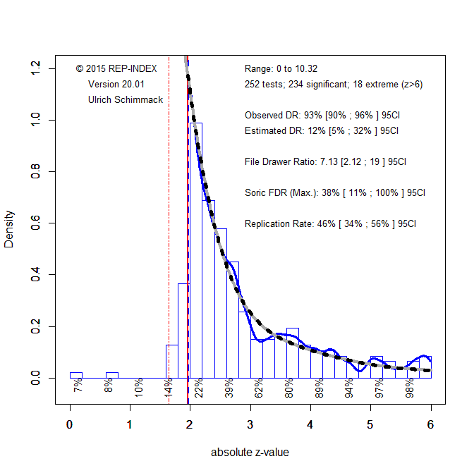
The figure shows the distribution of z-scores. As the book focussed on discoveries most test-statistics are significant with p < .05 (two-tailed, which corresponds to z = 1.96. The distribution of z-scores shows that these significant results were selected from a larger set of tests that produced non-significant results. The z-curve estimate is that the significant results are only 12% of all tests that were conducted. This is a problem.

Evidently, these results are selected from a larger set of studies that produced non-significant results. These results may not even have been published (publication bias). To estimate how replicable the significant results are, z-curve estimates the mean power of the significant results. This is similar to the R-Index, but the R-Index is only an approximate correction for information. Z-curve does properly correct for the selection for significance. The mean power is 46%, which implies that only half of the results would be replicated in exact replication studies. The success rate in actual replication studies is often lower and may be as low as the estimated discovery rate (Bartos & Schimmack, 2020). So, replicability is somewhere between 12% and 46%. Even if half of the results are replicable, we do not know which results are replicable and which one’s are not. The Chapter-based analyses provide some clues which findings may be less trustworthy (implicit priming) and which ones may be more trustworthy (overconfidence), but the main conclusion is that the empirical basis for claims in “Thinking: Fast and Slow” is shaky.

Conclusion

In conclusion, Daniel Kahneman is a distinguished psychologist who has made valuable contributions to the study of human decision making. His work with Amos Tversky was recognized with a Nobel Memorial Prize in Economics (APA). It is surely interesting to read what he has to say about psychological topics that range from cognition to well-being. However, his thoughts are based on a scientific literature with shaky foundations. Like everybody else in 2011, Kahneman trusted individual studies to be robust and replicable because they presented a statistically significant result. In hindsight it is clear that this is not the case. Narrative literature reviews of individual studies reflect scientists’ intuitions (Fast Thinking, System 1) as much or more than empirical findings. Readers of “Thinking: Fast and Slow” should read the book as a subjective account by an eminent psychologists, rather than an objective summary of scientific evidence. Moreover, ten years have passed and if Kahneman wrote a second edition, it would be very different from the first one. Chapters 3 and 4 would probably just be scrubbed from the book. But that is science. It does make progress, even if progress is often painfully slow in the softer sciences.

2016 Blogs

DECEMBER

12/31 ****
Review of an “eventful” 2016 (“Method Terrorists”)

12/6
A Forensic Analysis of Stapel: Fabrication or Falsification?

12/3
Replicability Analysis of Dijksterhuis’s “Enhancing Implicit Self-Esteem by Subliminal Evaluative Conditioning”

SEPTEMBER

9/13 ***
Critique of Finkel, Eastwick, & Reis’s article “Replicability and Other Features of a High-Quality Science: Toward a Balanced and Empirical Approach”

JUNE

6/30 ***
Wagenmaker’s Default Prior is Unrealistic

6/25 ****
A Principled Approach to Setting the Prior of the Null-Hypothesis

6/18 ***
What is the Difference between the Test of Excessive Significance and the Incredibility Index?

6/16 ****
The A Priori Probability of the Point Null-Hypothesis is not 50%

MAY

5/21
Replicability Report on Social Priming Studies with Mating Primes

5/18
Critique of Jeffrey N. Rouder, Richard D. Morey, and Eric-Jan Wagenmakers’s article “The Interplay between Subjectivity, Statistical Practice, and Psychological Science” 

5/9 ***
Questionable Research Practices Invalidate Bayes-Factors Just As Much as P-Values

APRIL

4/18 *****
Replicability Report of the Ego Depletion Literature

FEBRUARY

2/16 ****
Discussion of Sterling et al.’s (1995) Seminal Article on Inflated Success Rates in Psychological Science [also recommend reading the original article]

2/10
Replicability AudiT of a 10 Study Article by Adam D. Galinsky

2/9
A Replicability AudiT of Yaacov Trope’s Publications

2/3 ***
A Critique of Finkel, Eastwick, & Reis’s Views on the Replication Crisis

JANUARY

1/31 *****
Introduction to the R-Index
[The R-Index builds on the Incredibility Index, Schimmack (2012)]

1/31
Replicability Analysis of Damisch, Stoberock, & Mussweiler (2010)
[Anonymous Submission to R-Index Blog]

1/31
Replicability Analysis of Williams & Bargh (2008)

1/14 ***
Discussion of Hoenig and Heisey’s Critique of Observed Power Calculations

How replicable are statistically significant results in social psychology? A replication and extension of Motyl et al. (in press). 

Forthcoming article: 
Motyl, M., Demos, A. P., Carsel, T. S., Hanson, B. E., Melton, Z. J., Mueller, A. B., Prims, J., Sun, J., Washburn, A. N., Wong, K., Yantis, C. A., & Skitka, L. J. (in press). The state of social and personality science: Rotten to the core, not so bad, getting better, or getting worse? Journal of Personality and Social Psychology. (preprint)

Brief Introduction

Since JPSP published incredbile evidence for mental time travel (Bem, 2011), the credibility of social psychological research has been questioned.  There is talk of a crisis of confidence, a replication crisis, or a credibility crisis.  However, hard data on the credibility of empirical findings published in social psychology journals are scarce.

There have been two approaches to examine the credibility of social psychology.  One approach relies on replication studies.  Authors attempt to replicate original studies as closely as possible.  The most ambitious replication project was carried out by the Open Science Collaboration (Science, 2015) that replicated 1 study from 100 articles; 54 articles were classified as social psychology.   For original articles that reported a significant result, only a quarter replicated a significant result in the replication studies.  This estimate of replicability suggests that researches conduct many more studies than are published and that effect sizes in published articles are inflated by sampling error, which makes them difficult to replicate. One concern about the OSC results is that replicating original studies can be difficult.  For example, a bilingual study in California may not produce the same results as a bilingual study in Canada.  It is therefore possible that the poor outcome is partially due to problems of reproducing the exact conditions of original studies.

A second approach is to estimate replicability of published results using statistical methods.  The advantage of this approach is that replicabiliy estimates are predictions for exact replication studies of the original studies because the original studies provide the data for the replicability estimates.   This is the approach used by Motyl et al.

The authors sampled 30% of articles published in 2003-2004 (pre-crisis) and 2013-2014 (post-crisis) from four major social psychology journals (JPSP, PSPB, JESP, and PS).  For each study, coders identified one focal hypothesis and recorded the statistical result.  The bulk of the statistics were t-values from t-tests or regression analyses and F-tests from ANOVAs.  Only 19 statistics were z-tests.   The authors applied various statistical tests to the data that test for the presence of publication bias or whether the studies have evidential value (i.e., reject the null-hypothesis that all published results are false positives).  For the purpose of estimating replicability, the most important statistic is the R-Index.

The R-Index has two components.  First, it uses the median observed power of studies as an estimate of replicability (i.e., the percentage of studies that should produce a significant result if all studies were replicated exactly).  Second, it computes the percentage of studies with a significant result.  In an unbiased set of studies, median observed power and percentage of significant results should match.  Publication bias and questionable research practices will produce more significant results than predicted by median observed power.  The discrepancy is called the inflation rate.  The R-Index subtracts the inflation rate from median observed power because median observed power is an inflated estimate of replicability when bias is present.  The R-Index is not a replicability estimate.  That is, an R-Index of 30% does not mean that 30% of studies will produce a significant result.  However, a set of studies with an R-Index of 30 will have fewer successful replications than a set of studies with an R-Index of 80.  An exception is an R-Index of 50, which is equivalent with a replicability estimate of 50%.  If the R-Index is below 50, one would expect more replication failures than successes.

Motyl et al. computed the R-Index separately for the 2003/2004 and the 2013/2014 results and found “the R-index decreased numerically, but not statistically over time, from .62 [CI95% = .54, .68] in 2003-2004 to .52 [CI95% = .47, .56] in 2013-2014. This metric suggests that the field is not getting better and that it may consistently be rotten to the core.”

I think this interpretation of the R-Index results is too harsh.  I consider an R-Index below 50 an F (fail).  An R-Index in the 50s is a D, and an R-Index in the 60s is a C.  An R-Index greater than 80 is considered an A.  So, clearly there is a replication crisis, but social psychology is not rotten to the core.

The R-Index is a simple tool, but it is not designed to estimate replicability.  Jerry Brunner and I developed a method that can estimate replicability, called z-curve.  All test-statistics are converted into absolute z-scores and a kernel density distribution is fitted to the histogram of z-scores.  Then a mixture model of normal distributions is fitted to the density distribution and the means of the normal distributions are converted into power values. The weights of the components are used to compute the weighted average power. When this method is applied only to significant results, the weighted average power is the replicability estimate;  that is, the percentage of significant results that one would expect if the set of significant studies were replicated exactly.   Motyl et al. did not have access to this statistical tool.  They kindly shared their data and I was able to estimate replicability with z-curve.  For this analysis, I used all t-tests, F-tests, and z-tests (k = 1,163).   The Figure shows two results.  The left figure uses all z-scores greater than 2 for estimation (all values on the right side of the vertical blue line). The right figure uses only z-scores greater than 2.4.  The reason is that just-significant results may be compromised by questionable research methods that may bias estimates.

Motyl.2d0.2d4

The key finding is the replicability estimate.  Both estimations produce similar results (48% vs. 49%).  Even with over 1,000 observations there is uncertainty in these estimates and the 95%CI can range from 45 to 54% using all significant results.   Based on this finding, it is predicted that about half of these results would produce a significant result again in a replication study.

However, it is important to note that there is considerable heterogeneity in replicability across studies.  As z-scores increase, the strength of evidence becomes stronger, and results are more likely to replicate.  This is shown with average power estimates for bands of z-scores at the bottom of the figure.   In the left figure,  z-scores between 2 and 2.5 (~ .01 < p < .05) have only a replicability of 31%, and even z-scores between 2.5 and 3 have a replicability below 50%.  It requires z-scores greater than 4 to reach a replicability of 80% or more.   Similar results are obtained for actual replication studies in the OSC reproducibilty project.  Thus, researchers should take the strength of evidence of a particular study into account.  Studies with p-values in the .01 to .05 range are unlikely to replicate without boosting sample sizes.  Studies with p-values less than .001 are likely to replicate even with the same sample size.

Independent Replication Study 

Schimmack and Brunner (2016) applied z-curve to the original studies in the OSC reproducibility project.  For this purpose, I coded all studies in the OSC reproducibility project.  The actual replication project often picked one study from articles with multiple studies.  54 social psychology articles reported 173 studies.   The focal hypothesis test of each study was used to compute absolute z-scores that were analyzed with z-curve.

OSC.soc

The two estimation methods (using z > 2.0 or z > 2.4) produced very similar replicability estimates (53% vs. 52%).  The estimates are only slightly higher than those for Motyl et al.’s data (48% & 49%) and the confidence intervals overlap.  Thus, this independent replication study closely replicates the estimates obtained with Motyl et al.’s data.

Automated Extraction Estimates

Hand-coding of focal hypothesis tests is labor intensive and subject to coding biases. Often studies report more than one hypothesis test and it is not trivial to pick one of the tests for further analysis.  An alternative approach is to automatically extract all test statistics from articles.  This makes it also possible to base estimates on a much larger sample of test results.  The downside of automated extraction is that articles also report statistical analysis for trivial or non-critical tests (e.g., manipulation checks).  The extraction of non-significant results is irrelevant because they are not used by z-curve to estimate replicability.  I have reported the results of this method for various social psychology journals covering the years from 2010 to 2016 and posted powergraphs for all journals and years (2016 Replicability Rankings).   Further analyses replicated the results from the OSC reproducibility project that results published in cognitive journals are more replicable than those published in social journals.  The Figure below shows that the average replicability estimate for social psychology is 61%, with an encouraging trend in 2016.  This estimate is about 10% above the estimates based on hand-coded focal hypothesis tests in the two datasets above.  This discrepancy can be due to the inclusion of less original and trivial statistical tests in the automated analysis.  However, a 10% difference is not a dramatic difference.  Neither 50% nor 60% replicability justify claims that social psychology is rotten to the core, nor do they meet the expectation that researchers should plan studies with 80% power to detect a predicted effect.

replicability-cog-vs-soc

Moderator Analyses

Motyl et al. (in press) did extensive coding of the studies.  This makes it possible to examine potential moderators (predictors) of higher or lower replicability.  As noted earlier, the strength of evidence is an important predictor.  Studies with higher z-scores (smaller p-values) are, on average, more replicable.  The strength of evidence is a direct function of statistical power.  Thus, studies with larger population effect sizes and smaller sampling error are more likely to replicate.

It is well known that larger samples have less sampling error.  Not surprisingly, there is a correlation between sample size and the absolute z-scores (r = .3).  I also examined the R-Index for different ranges of sample sizes.  The R-Index was the lowest for sample sizes between N = 40 and 80 (R-Index = 43), increased for N = 80 to 200 (R-Index = 52) and further for sample sizes between 200 and 1,000 (R-Index = 69).  Interestingly, the R-Index for small samples with N < 40 was 70.  This is explained by the fact that research designs also influence replicability and that small samples often use more powerful within-subject designs.

A moderator analysis with design as moderator confirms this.  The R-Indices for between-subject designs is the lowest (R-Index = 48) followed by mixed designs (R-Index = 61) and then within-subject designs (R-Index = 75).  This pattern is also found in the OSC reproducibility project and partially accounts for the higher replicability of cognitive studies, which often employ within-subject designs.

Another possibility is that articles with more studies package smaller and less replicable studies.  However,  number of studies in an article was not a notable moderator:  1 study R-Index = 53, 2 studies R-Index = 51, 3 studies R-Index = 60, 4 studies R-Index = 52, 5 studies R-Index = 53.

Conclusion 

Motyl et al. (in press) coded a large and representative sample of results published in social psychology journals.  Their article complements results from the OSC reproducibility project that used actual replications, but a much smaller number of studies.  The two approaches produce different results.  Actual replication studies produced only 25% successful replications.  Statistical estimates of replicability are around 50%.   Due to the small number of actual replications in the OSC reproducibility project, it is important to be cautious in interpreting the differences.  However, one plausible explanation for lower success rates in actual replication studies is that it is practically impossible to redo a study exactly.  This may even be true when researchers conduct three similar studies in their own lab and only one of these studies produces a significant result.  Some non-random, but also not reproducible, factor may have helped to produce a significant result in this study.  Statistical models assume that we can redo a study exactly and may therefore overestimate the success rate for actual replication studies.  Thus, the 50% estimate is an optimistic estimate for the unlikely scenario that a study can be replicated exactly.  This means that even though optimists may see the 50% estimate as “the glass half full,” social psychologists need to increase statistical power and pay more attention to the strength of evidence of published results to build a robust and credible science of social behavior.


Hidden Figures: Replication Failures in the Stereotype Threat Literature

In the past five years, it has become apparent that many classic and important findings in social psychology fail to replicate (Schimmack, 2016).  The replication crisis is often considered a new phenomenon, but failed replications are not entirely new.  Sometimes these studies have simply been ignored.  These studies deserve more attention and need to be reevaluated in the context of the replication crisis in social psychology.

In the past, failed replications were often dismissed because seminal articles were assumed to provide robust empirical support for a phenomenon, especially if an article presented multiple studies. The chance of reporting a false positive results in a multiple study article is low because the risk of a false positive decreases exponentially (Schimmack, 2012). However, the low risk of a false positive is illusory if authors only publish studies that worked. In this case, even false positives can be supported by significant results in multiple studies, as demonstrated in the infamous ESP study by Bem (2011).  As a result, publication bias undermines the reporting of statistical significance as diagnostic information about the risk of false positives (Sterling, 1959) and many important theories in social psychology rest on shaky empirical foundations that need to be reexamined.

Research on stereotype threat and women’s performance on math tests is one example where publication bias undermines the findings in a seminal study that produced a large literature of studies on gender differences in math performance. After correcting for publication bias, this literature shows very little evidence that stereotype threat has a notable and practically significant effect on women’s math performance (Flore & Wicherts, 2014).

Another important line of research has examined the contribution of stereotype threat to differences between racial groups on academic performance tests.  This blog post examines the strength of the empirical evidence for stereotype threat effects in the seminal article by Steele and Aronson (1995). This article is currently the 12th most cited article in the top journal for social psychology, Journal of Personality and Social Psychology (2,278 citations so far).

According to the abstract, “stereotype threat is being at risk of confirming, as self-characteristic, a negative stereotype about one’s group.” Studies 1 and 2 showed that “reflecting the pressure of this vulnerability, Blacks underperformed in relation to Whites in the ability-diagnostic condition but not in the nondiagnostic condition (with Scholastic Aptitude Tests controlled).”  “Study 3 validated that ability-diagnosticity cognitively activated the racial stereotype in these participants and motivated them not to conform to it, or to be judged by it.”  “Study 4 showed that mere salience of the stereotype could impair Blacks’ performance even when the test was not
ability diagnostic.”

The results of Study 4 motivated Stricker and colleagues to examine the influence of stereotype-treat on test performance in a real-world testing situation.  These studies had large samples and were not limited to students at Stanford. One study was reported in a College Board Report (Stricker and Ward, 1998).   Another two studies were published in the Journal of Applied Social Psychology (Stricker & Ward, 2004).  This article received only 52 citations, although it reported two studies with an experimental manipulation of stereotype threat in a real assessment context.  One group of participants were asked about their gender or ethnicity before the text, the other group did not receive these questions.  As noted in the abstract, neither the inquiry about race, nor about gender, had a significant effect on test performance. In short, this study failed to replicate Study 4 of the classic and widely cited article by Steele and Aronson.

Stricker and Ward’s Abstract
Steele and Aronson (1995) found that the performance of Black research participants on
ability test items portrayed as a problem-solving task, in laboratory experiments, was affected adversely when they were asked about their ethnicity. This outcome was attributed to stereotype threat: Performance was disrupted by participants’ concerns about fulfilling the negative stereotype concerning Black people’s intellectual ability. The present field experiments extended that research to other ethnic groups and to males and females taking operational tests. The experiments evaluated the effects of inquiring about ethnicity and gender on the performance of students taking 2 standardized tests-the Advanced Placement Calculus AB Examination, and the Computerized Placement Tests-in actual test administrations. This inquiry did not have any effects on the test performance of Black, female, or other subgroups of students that were both statistically and practically significant.

The article also mentions a personal communication with Steele, in which Steele mentions an unpublished study that also failed to demonstrate the effect under similar conditions.

“In fact, Steele found in an unpublished pilot study that inquiring about ethnicity did not affect Black participants’ performance when the task was described as diagnostic of their ability (C. M. Steele, personal communication, May 2 1, 1997), in contrast to the
substantial effect of inquiring when the task was described as nondiagnostic.”

A substantive interpretation of this finding is that inquires about race or gender do not produce stereotype threat effects when a test is diagnostic because a diagnostic test already activates stereotype threat.  However, if this were a real moderator, it would be important to document this fact and it is not clear why this finding obtained in an earlier study by Steele remained unpublished. Moreover, it is premature to interpret the significant result in the published study with a non-diagnostic task and the non-significant result in an unpublished study with a diagnostic task as evidence that diagnosticity moderates the effect of the stereotype-threat manipulation. A proper test of this moderator hypothesis would require the demonstration of a three-way interaction between race, inquiry about race, and diagnosticity. Absent this evidence, it remains possible that diagnosticity is not a moderator and that the published result is a false positive (or a positive result with an inflated effect size estimate). In contrast, there appears to be consistent evidence that inquiries about race or gender before a real assessment of academic performance does not influence performance. This finding is not widely publicized, but is important for a better understanding of performance differences in real world settings.

The best way to examine the replicability of Steele and Aronson’s seminal finding with non-diagnostic tasks would be to conduct an exact replication study.  However, exact replication studies are difficult and costly.  An alternative is to examine the robustness of the published results by taking a closer look at the strength of the statistical results reported by Steele and Aronson, using modern statistical tests of publication bias and statistical power like the R-Index (Schimmack, 2014) and the Test of Insufficient Variance (TIVA, Schimmack, 2014).

Replicability Analysis of Steele and Aronson’s four studies

Study 1. The first study had a relatively large sample of N = 114 participants, but it is not clear how many of the participants were White or Black.  The study also had a 2 x 3 design, which leaves less than 20 participants per condition.   The study produced a significant main effect of condition, F(2, 107) = 4.74, and race, F(1,107) = 5.22, but the critical condition x race interaction was not significant (reported as p > .19).   However, a specific contrast showed significant differences between Black participants in the diagnostic condition and the non-diagnostic condition, t(107) = 2.88, p = .005, z = 2.82.  The authors concluded “in sum, then, the hypothesis was supported by the pattern of contrasts, but when tested over the whole design, reached only marginal significance” (p. 800).  In other words, Study 1 provided only weak support for the stereotype threat hypothesis.

Study 2. Study 2 eliminated one of the three experimental conditions. Participants were 20 Black and 20 White participants. This means there were only 10 participants in each condition of a 2 x 2 design. The degrees of freedom further indicate that the actual sample size was only 38 participants. Given the weak evidence in Study 1, there is no justification for a reduction in the number of participants per cell, although the difficulty of recruiting Black participants at Stanford may explain this inadequate sample size. Nevertheless, the study showed a significant interaction between race and test description, F(1,35) = 8.07, p = .007. The study also replicated the contrast from Study 1 that Black participants in the diagnostic condition performed significantly worse than Black participants in the non-diagnostic group, t(35) = 2.38, p = .023, z = 2.28.

Studies 1 and 2 are close replications of each other.  The consistent finding across the two studies that supports stereotype-treat theory is the finding that merely changing the description of an assessment task changes Black participants performance, as revealed by significant differences between the diagnostic and non-diagnostic condition in both studies.  The problem is that both studies had small numbers of Black participants and that small samples have low power to produce significant results. As a result, it is unlikely that a pair of studies would produce significant results in both studies.

Observed power  in the two studies is .81 and .62 with median observed power of .71. Thus, the actual success rate of 100% (2 out of 2 significant results) is 29 percentage points higher than the expected success rate. Moreover, when inflation is evident, median observed power is also inflated. To correct for this inflation, the Replicability-Index (R-Index) subtracts inflation from median observed power, which yields an R-Index of 42.  Any value below 50 is considered unacceptably low and I give it a letter grade F, just like students at American Universities receive an F for exams with less than 50% correct answers.  This does not mean that stereotype threat is not a valid theory or that there was no real effect in this pair of studies. It simply means that the evidence in this highly cited article is insufficient to make strong claims about the causes of Black’s performance on academic tests.

The Test of Insufficient Variance (TIVA) provides another way to examine published results.  Test statistics like t-values vary considerably from study to study even if the exact same study is conducted twice (or if one larger sample is randomly split into two sub-samples).  When test-statistics are converted into z-scores, sampling error (the random variability from sample to sample) follows approximately a standard normal distribution with a variance of 1.  If the variance is considerably smaller than 1, it suggests that the reported results represent a selected sample. Often the selection is a result of publication bias.  Applying TIVA to the pair of studies, yields a variance of Var(z) = 0.15.  As there are only two studies, it is possible that this outcome occurred by chance, p = .300, and it does not imply intentional selection for significance or other questionable research practices.  Nevertheless, it suggests that future replication studies will be more variable and produce some non-significant results.

In conclusion, the evidence presented in the first two studies is weaker than we might assume if we focused only on the fact that both studies produced significant contrasts. Given publication bias, the fact that both studies reported significant results provides no empirical evidence because virtually all published studies report significant results. The R-Index quantifies the strength of evidence for an effect while taking the influence of publication bias into account and it shows that the two studies with small samples provide only weak evidence for an effect.

Study 3.  This study did not examine performance. The aim was to demonstrate activation of stereotype threat with a sentence completion task.  The sample size of 68 participants  (35 Black, 33 White) implied that only 11 or 12 participants were assigned to one of the six cells in a 2 (race) by 3 (task description) design. The study produced main effects for race and condition, but most importantly it produced a significant interaction effect, F(2,61) = 3.30, p = .044.  In addition, Black participants in the diagnostic condition had more stereotype-related associations than Black participants in the non-diagnostic condition, t(61) = 3.53,

Study 4.  This study used inquiry about race to induce stereotype-threat. Importantly, the task was described as non-diagnostic (as noted earlier, a similar study produced no significant results when the task was described as diagnostic).  The design was a 2 x 2 design with 47 participants, which means only 11 or 12 participants were allocated to the four conditions.  The degrees of freedom indicated that cell frequencies were even lower. The study produced a significant interaction effect, F(1,39) = 7.82, p = .008.  The study also produced a significant contrast between Blacks in the race-prime condition and the no-prime condition, t(39) = 2.43, p = .020.

The contrast effect in Study 3 is strong, but it is not a performance measure.  If stereotype threat mediates the effect of task characteristics and performance, we would expect a stronger effect on the measure of the mediator than on the actual outcome of interest, task performance.  The key aim of stereotype threat theory is to explain differences in performance.  With a focus on performance outcomes, it is possible to examine the R-Index and TIVA of Studies 1, 2, and 4.  All three studies reported significant contrasts between Black students randomly assigned to two groups that were expected to show performance differences (Table 1).

Table 1

Study Test Statistic p-value z-score obs.pow
Study 1 t(107) = 2.88 0.005 2.82 0.81
Study 2 t(35)=2.38 0.023 2.28 0.62
Study 4 t(39) = 2.43 0.020 2.33 0.64

Median observed power is 64 and the R-Index is well below 50, 64 – 36 = 28 (F).  The variance in z-scores is Var(z) = 0.09, p = .086.  These results cast doubt about the replicability of the performance effects reported in Steele and Aronson’s seminal stereotype threat article.

Conclusion

Racial stereotypes and racial disparities are an important social issue.  Social psychology aims and promises to contribute to the understanding of this issue by conducting objective, scientific studies that can inform our understanding of these issues.  In order to live up to these expectations, social psychology has to follow the rules of science and listen to the data.  Just like it is important to get the numbers right to send men and women into space (and bring them back), it is important to get the numbers right when we use science to understand women and men on earth.  Unfortunately, social psychologists have not followed the examples of astronomers and the numbers do not add up.

The three African American women, features in this years movie “Hidden Figures”***,  Katherine Johnson, Dorothy Vaughan, and Mary Jackson might not approve of the casual way social psychologists use numbers in their research, especially the wide-spread practice of hiding numbers that do not match expectations.  No science that wants to make a real-world contribution can condone this practice.  It is also not acceptable to simply ignore published results from well-conducted studies with large samples that challenge a prominent theory.

Surely, the movie Hidden Figures dramatized some of the experiences of Black women at NASA, but there is little doubt that Katherine Johnson, Dorothy Vaughan, and Mary Jackson encountered many obstacles that might be considered stereotype threatening situations.  Yet, they prevailed and they paved the way for future generations of stereotyped groups.  Understanding racial and gender bias and performance differences remains an important issue and that is the reason why it is important to shed a light on hidden numbers and put simplistic theories under the microscope. Stereotype threat is too often used as a simple explanation that avoids tackling deeper and more difficult issues that cannot be easily studied in a quick laboratory experiment with undergraduate students at top research universities.  It is time for social psychologists to live up to its promises by tackling real world issues with research designs that have real world significance that produce real evidence using open and transparent research practices.

————————————————————————————————————————————

*** If you haven’t seen the movie, I highly recommend it.


How Selection for Significance Influences Observed Power

Two years ago, I posted an Excel spreadsheet to help people to understand the concept of true power, observed power, and how selection for significance inflates observed power. Two years have gone by and I have learned R. It is time to update the post.

There is no mathematical formula to correct observed power for inflation to solve for true power. This was partially the reason why I created the R-Index, which is an index of true power, but not an estimate of true power.  This has led to some confusion and misinterpretation of the R-Index (Disjointed Thought blog post).

However, it is possible to predict median observed power given true power and selection for statistical significance.  To use this method for real data with observed median power of only significant results, one can simply generate a range of true power values, generate the predicted median observed power and then pick the true power value with the smallest discrepancy between median observed power and simulated inflated power estimates. This approach is essentially the same as the approach used by pcurve and puniform, which only
differ in the criterion that is being minimized.

Here is the r-code for the conversion of true.power into the predicted observed power after selection for significance.

true.power = seq(.01,.99,.01)
obs.pow = pnorm(qnorm(true.power/2+(1-true.power),qnorm(true.power,z.crit)),z.crit)

And here is a pretty picture of the relationship between true power and inflated observed power.  As we can see, there is more inflation for low true power because observed power after selection for significance has to be greater than 50%.  With alpha = .05 (two-tailed), when the null-hypothesis is true, inflated observed power is 61%.   Thus, an observed median power of 61% for only significant results supports the null-hypothesis.  With true power of 50%, observed power is inflated to 75%.  For high true power, the inflation is relatively small. With the recommended true power of 80%, median observed power for only significant results is 86%.

inflated-mop

Observed power is easy to calculate from reported test statistics. The first step is to compute the exact two-tailed p-value.  These p-values can then be converted into observed power estimates using the standard normal distribution.

z.crit = qnorm(.975)
Obs.power = pnorm(qnorm(1-p/2),z.crit)

If there is selection for significance, you can use the previous formula to convert this observed power estimate into an estimate of true power.

This method assumes that (a) significant results are representative of the distribution and there are no additional biases (no p-hacking) and (b) all studies have the same or similar power.  This method does not work for heterogeneous sets of studies.

P.S.  It is possible to proof the formula that transforms true power into median observed power.  Another way to verify that the formula is correct is to confirm the predicted values with a simulation study.

Here is the code to run the simulation study:

n.sim = 100000
z.crit = qnorm(.975)
true.power = seq(.01,.99,.01)
obs.pow.sim = c()
for (i in 1:length(true.power)) {
z.sim = rnorm(n.sim,qnorm(true.power[i],z.crit))
med.z.sig = median(z.sim[z.sim > z.crit])
obs.pow.sim = c(obs.pow.sim,pnorm(med.z.sig,z.crit))
}
obs.pow.sim

obs.pow = pnorm(qnorm(true.power/2+(1-true.power),qnorm(true.power,z.crit)),z.crit)
obs.pow
cbind(true.power,obs.pow.sim,obs.pow)
plot(obs.pow.sim,obs.pow)


Reconstruction of a Train Wreck: How Priming Research Went off the Rails

This blog post focusses on Chapter 4 about Implicit Priming in Kahneman’s book “Thinking” Fast and Slow.”  A review of the book and other chapters can be found here: https://replicationindex.com/2020/12/30/a-meta-scientific-perspective-on-thinking-fast-and-slow/

Daniel Kahneman’s response to this blog post:
https://replicationindex.com/2017/02/02/reconstruction-of-a-train-wreck-how-priming-research-went-of-the-rails/comment-page-1/#comment-1454

Authors:  Ulrich Schimmack, Moritz Heene, and Kamini Kesavan

Abstract:
We computed the R-Index for studies cited in Chapter 4 of Kahneman’s book “Thinking Fast and Slow.” This chapter focuses on priming studies, starting with John Bargh’s study that led to Kahneman’s open email.  The results are eye-opening and jaw-dropping.  The chapter cites 12 articles and 11 of the 12 articles have an R-Index below 50.  The combined analysis of 31 studies reported in the 12 articles shows 100% significant results with average (median) observed power of 57% and an inflation rate of 43%.  The R-Index is 14. This result confirms Kahneman’s prediction that priming research is a train wreck and readers of his book “Thinking Fast and Slow” should not consider the presented studies as scientific evidence that subtle cues in their environment can have strong effects on their behavior outside their awareness.

Introduction

In 2011, Nobel Laureate Daniel Kahneman published a popular book, “Thinking Fast and Slow”, about important finding in social psychology.

In the same year, questions about the trustworthiness of social psychology were raised.  A Dutch social psychologist had fabricated data. Eventually over 50 of his articles would be retracted.  Another social psychologist published results that appeared to demonstrate the ability to foresee random future events (Bem, 2011). Few researchers believed these results and statistical analysis suggested that the results were not trustworthy (Francis, 2012; Schimmack, 2012).  Psychologists started to openly question the credibility of published results.

In the beginning of 2012, Doyen and colleagues published a failure to replicate a prominent study by John Bargh that was featured in Daniel Kahneman’s book.  A few month later, Daniel Kahneman distanced himself from Bargh’s research in an open email addressed to John Bargh (Young, 2012):

“As all of you know, of course, questions have been raised about the robustness of priming results…. your field is now the poster child for doubts about the integrity of psychological research… people have now attached a question mark to the field, and it is your responsibility to remove it… all I have personally at stake is that I recently wrote a book that emphasizes priming research as a new approach to the study of associative memory…Count me as a general believer… My reason for writing this letter is that I see a train wreck looming.”

Five years later, Kahneman’s concerns have been largely confirmed. Major studies in social priming research have failed to replicate and the replicability of results in social psychology is estimated to be only 25% (OSC, 2015).

Looking back, it is difficult to understand the uncritical acceptance of social priming as a fact.  In “Thinking Fast and Slow” Kahneman wrote “disbelief is not an option. The results are not made up, nor are they statistical flukes. You have no choice but to accept that the major conclusions of these studies are true.”

Yet, Kahneman could have seen the train wreck coming. In 1971, he co-authored an article about scientists’ “exaggerated confidence in the validity of conclusions based on small samples” (Tversky & Kahneman, 1971, p. 105).  Yet, many of the studies described in Kahneman’s book had small samples.  For example, Bargh’s priming study used only 30 undergraduate students to demonstrate the effect.

Replicability Index

Small samples can be sufficient to detect large effects. However, small effects require large samples.  The probability of replicating a published finding is a function of sample size and effect size.  The Replicability Index (R-Index) makes it possible to use information from published results to predict how replicable published results are.

Every reported test-statistic can be converted into an estimate of power, called observed power. For a single study, this estimate is useless because it is not very precise. However, for sets of studies, the estimate becomes more precise.  If we have 10 studies and the average power is 55%, we would expect approximately 5 to 6 studies with significant results and 4 to 5 studies with non-significant results.

If we observe 100% significant results with an average power of 55%, it is likely that studies with non-significant results are missing (Schimmack, 2012).  There are too many significant results.  This is especially true because average power is also inflated when researchers report only significant results. Consequently, the true power is even lower than average observed power.  If we observe 100% significant results with 55% average powered power, power is likely to be less than 50%.

This is unacceptable. Tversky and Kahneman (1971) wrote “we refuse to believe that a serious investigator will knowingly accept a .50 risk of failing to confirm a valid research hypothesis.”

To correct for the inflation in power, the R-Index uses the inflation rate. For example, if all studies are significant and average power is 75%, the inflation rate is 25% points.  The R-Index subtracts the inflation rate from average power.  So, with 100% significant results and average observed power of 75%, the R-Index is 50% (75% – 25% = 50%).  The R-Index is not a direct estimate of true power. It is actually a conservative estimate of true power if the R-Index is below 50%.  Thus, an R-Index below 50% suggests that a significant result was obtained only by capitalizing on chance, although it is difficult to quantify by how much.

How Replicable are the Social Priming Studies in “Thinking Fast and Slow”?

Chapter 4: The Associative Machine

4.1.  Cognitive priming effect

In the 1980s, psychologists discovered that exposure to a word causes immediate and measurable changes in the ease with which many related words can be evoked.

[no reference provided]

4.2.  Priming of behavior without awareness

Another major advance in our understanding of memory was the discovery that priming is not restricted to concepts and words. You cannot know this from conscious experience, of course, but you must accept the alien idea that your actions and your emotions can be primed by events of which you are not even aware.

“In an experiment that became an instant classic, the psychologist John Bargh and his collaborators asked students at New York University—most aged eighteen to twenty-two—to assemble four-word sentences from a set of five words (for example, “finds he it yellow instantly”). For one group of students, half the scrambled sentences contained words associated with the elderly, such as Florida, forgetful, bald, gray, or wrinkle. When they had completed that task, the young participants were sent out to do another experiment in an office down the hall. That short walk was what the experiment was about. The researchers unobtrusively measured the time it took people to get from one end of the corridor to the other.”

“As Bargh had predicted, the young people who had fashioned a sentence from words with an elderly theme walked down the hallway significantly more slowly than the others. walking slowly, which is associated with old age.”

“All this happens without any awareness. When they were questioned afterward, none of the students reported noticing that the words had had a common theme, and they all insisted that nothing they did after the first experiment could have been influenced by the words they had encountered. The idea of old age had not come to their conscious awareness, but their actions had changed nevertheless.“

[John A. Bargh, Mark Chen, and Lara Burrows, “Automaticity of Social Behavior: Direct Effects of Trait Construct and Stereotype Activation on Action,” Journal of Personality and Social Psychology 71 (1996): 230–44.]

t(28)=2.860.0082.660.76
t(28)=2.160.0392.060.54

MOP = .65, Inflation = .35, R-Index = .30

4.3.  Reversed priming: Behavior primes cognitions

“The ideomotor link also works in reverse. A study conducted in a German university was the mirror image of the early experiment that Bargh and his colleagues had carried out in New York.”

“Students were asked to walk around a room for 5 minutes at a rate of 30 steps per minute, which was about one-third their normal pace. After this brief experience, the participants were much quicker to recognize words related to old age, such as forgetful, old, and lonely.”

“Reciprocal priming effects tend to produce a coherent reaction: if you were primed to think of old age, you would tend to act old, and acting old would reinforce the thought of old age.”

t(18)=2.100.0501.960.50
t(35)=2.100.0432.020.53
t(31)=2.500.0182.370.66

MOP = .53, Inflation = .47, R-Index = .06

4.4.  Facial-feedback hypothesis (smiling makes you happy)

“Reciprocal links are common in the associative network. For example, being amused tends to make you smile, and smiling tends to make you feel amused….”

“College students were asked to rate the humor of cartoons from Gary Larson’s The Far Side while holding a pencil in their mouth. Those who were “smiling” (without any awareness of doing so) found the cartoons funnier than did those who were “frowning.”

[“Inhibiting and Facilitating Conditions of the Human Smile: A Nonobtrusive Test of the Facial Feedback Hypothesis,” Journal of Personality and Social Psychology 54 (1988): 768–77.]

The authors used the more liberal and unconventional criterion of p < .05 (one-tailed), z = 1.65, as a criterion for significance. Accordingly, we adjusted the R-Index analysis and used 1.65 as the criterion value.

t(89)=1.850.0341.830.57
t(75)=1.780.0341.830.57

MOP = .57, Inflation = .43, R-Index = .14

These results could not be replicated in a large replication effort with 17 independent labs. Not a single lab produced a significant result and even a combined analysis failed to show any evidence for the effect.

4.5. Automatic Facial Responses

In another experiment, people whose face was shaped into a frown (by squeezing their eyebrows together) reported an enhanced emotional response to upsetting pictures—starving children, people arguing, maimed accident victims.

[Ulf Dimberg, Monika Thunberg, and Sara Grunedal, “Facial Reactions to

Emotional Stimuli: Automatically Controlled Emotional Responses,” Cognition and Emotion, 16 (2002): 449–71.]

The description in the book does not match any of the three studies reported in this article. The first two studies examined facial muscle movements in response to pictures of facial expressions (smiling or frowning faces).  The third study used emotional pictures of snakes and flowers. We might consider the snake pictures as being equivalent to pictures of starving children or maimed accident victims.  Participants were also asked to frown or to smile while looking at the pictures. However, the dependent variable was not how they felt in response to pictures of snakes, but rather how their facial muscles changed.  Aside from a strong effect of instructions, the study also found that the emotional picture had an automatic effect on facial muscles.  Participants frowned more when instructed to frown and looking at a snake picture than when instructed to frown and looking at a picture of a flower. “This response, however, was larger to snakes than to flowers as indicated by both the Stimulus factor, F(1, 47) = 6.66, p < .02, and the Stimulus 6 Interval factor, F(1, 47) = 4.30, p < .05.”  (p. 463). The evidence for smiling was stronger. “The zygomatic major muscle response was larger to flowers than to snakes, which was indicated by both the Stimulus factor, F(1, 47) = 18.03, p < .001, and the Stimulus 6 Interval factor, F(1, 47) = 16.78, p < .001.”  No measures of subjective experiences were included in this study.  Therefore, the results of this study provide no evidence for Kahneman’s claim in the book and the results of this study are not included in our analysis.

4.6.  Effects of Head-Movements on Persuasion

“Simple, common gestures can also unconsciously influence our thoughts and feelings.”

“In one demonstration, people were asked to listen to messages through new headphones. They were told that the purpose of the experiment was to test the quality of the audio equipment and were instructed to move their heads repeatedly to check for any distortions of sound. Half the participants were told to nod their head up and down while others were told to shake it side to side. The messages they heard were radio editorials.”

“Those who nodded (a yes gesture) tended to accept the message they heard, but those who shook their head tended to reject it. Again, there was no awareness, just a habitual connection between an attitude of rejection or acceptance and its common physical expression.”

F(2,66)=44.700.0007.221.00

MOP = 1.00, Inflation = .00,  R-Index = 1.00

[Gary L. Wells and Richard E. Petty, “The Effects of Overt Head Movements on Persuasion: Compatibility and Incompatibility of Responses,” Basic and Applied Social Psychology, 1, (1980): 219–30.]

4.7   Location as Prime

“Our vote should not be affected by the location of the polling station, for example, but it is.”

“A study of voting patterns in precincts of Arizona in 2000 showed that the support for propositions to increase the funding of schools was significantly greater when the polling station was in a school than when it was in a nearby location.”

“A separate experiment showed that exposing people to images of classrooms and school lockers also increased the tendency of participants to support a school initiative. The effect of the images was larger than the difference between parents and other voters!”

[Jonah Berger, Marc Meredith, and S. Christian Wheeler, “Contextual Priming: Where People Vote Affects How They Vote,” PNAS 105 (2008): 8846–49.]

z = 2.100.0362.100.56
p = .050.0501.960.50

MOP = .53, Inflation = .47, R-Index = .06

4.8  Money Priming

“Reminders of money produce some troubling effects.”

“Participants in one experiment were shown a list of five words from which they were required to construct a four-word phrase that had a money theme (“high a salary desk paying” became “a high-paying salary”).”

“Other primes were much more subtle, including the presence of an irrelevant money-related object in the background, such as a stack of Monopoly money on a table, or a computer with a screen saver of dollar bills floating in water.”

“Money-primed people become more independent than they would be without the associative trigger. They persevered almost twice as long in trying to solve a very difficult problem before they asked the experimenter for help, a crisp demonstration of increased self-reliance.”

“Money-primed people are also more selfish: they were much less willing to spend time helping another student who pretended to be confused about an experimental task. When an experimenter clumsily dropped a bunch of pencils on the floor, the participants with money (unconsciously) on their mind picked up fewer pencils.”

“In another experiment in the series, participants were told that they would shortly have a get-acquainted conversation with another person and were asked to set up two chairs while the experimenter left to retrieve that person. Participants primed by money chose to stay much farther apart than their nonprimed peers (118 vs. 80 centimeters).”

“Money-primed undergraduates also showed a greater preference for being alone.”

[Kathleen D. Vohs, “The Psychological Consequences of Money,” Science 314 (2006): 1154–56.]

F(2,49)=3.730.0312.160.58
t(35)=2.030.0501.960.50
t(37)=2.060.0461.990.51
t(42)=2.130.0392.060.54
F(2,32)=4.340.0212.300.63
t(38)=2.130.0402.060.54
t(33)=2.370.0242.260.62
F(2,58)=4.040.0232.280.62
chi^2(2)=10.100.0062.730.78

MOP = .58, Inflation = .42, R-Index = .16

4.9  Death Priming

“The evidence of priming studies suggests that reminding people of their mortality increases the appeal of authoritarian ideas, which may become reassuring in the context of the terror of death.”

The cited article does not directly examine this question.  The abstract states that “three experiments were conducted to test the hypothesis, derived from terror management theory, that reminding people of their mortality increases attraction to those who consensually validate their beliefs and decreases attraction to those who threaten their beliefs” (p. 308).  Study 2 found no general effect of death priming. Rather, the effect was qualified by authoritarianism. Mortality salience enhanced the rejection of dissimilar others in Study 2 only among high authoritarian subjects.” (p. 314), based on a three-way interaction with F(1,145) = 4.08, p = .045.  We used the three-way interaction for the computation of the R-Index.  Study 1 reported opposite effects for ratings of Christian targets, t(44) = 2.18, p = .034 and Jewish targets, t(44)= 2.08, p = .043. As these tests are dependent, only one test could be used, and we chose the slightly stronger result.  Similarly, Study 3 reported significantly more liking of a positive interviewee and less liking of a negative interviewee, t(51) = 2.02, p = .049 and t(49) = 2.42, p = .019, respectively. We chose the stronger effect.

[Jeff Greenberg et al., “Evidence for Terror Management Theory II: The Effect of Mortality Salience on Reactions to Those Who Threaten or Bolster the Cultural Worldview,” Journal of Personality and Social Psychology]

t(44)=2.180.0352.110.56
F(1,145)=4.080.0452.000.52
t(49)=2.420.0192.340.65

MOP = .56, Inflation = .44, R-Index = .12

4.10  The “Lacy Macbeth Effect”

“For example, consider the ambiguous word fragments W_ _ H and S_ _ P. People who were recently asked to think of an action of which they are ashamed are more likely to complete those fragments as WASH and SOAP and less likely to see WISH and SOUP.”

“Furthermore, merely thinking about stabbing a coworker in the back leaves people more inclined to buy soap, disinfectant, or detergent than batteries, juice, or candy bars. Feeling that one’s soul is stained appears to trigger a desire to cleanse one’s body, an impulse that has been dubbed the “Lady Macbeth effect.”

[Lady Macbeth effect”: Chen-Bo Zhong and Katie Liljenquist, “Washing Away Your Sins:

Threatened Morality and Physical Cleansing,” Science 313 (2006): 1451–52.]

F(1,58)=4.260.0442.020.52
F(1,25)=6.990.0142.460.69

MOP = .61, Inflation = .39, R-Index = .22

The article reports two more studies that are not explicitly mentioned, but are used as empirical support for the Lady Macbeth effect. As the results of these studies were similar to those in the mentioned studies, including these tests in our analysis does not alter the conclusions.

chi^2(1)=4.570.0332.140.57
chi^2(1)=5.020.0252.240.61

MOP = .59, Inflation = .41, R-Index = .18

4.11  Modality Specificity of the “Lacy Macbeth Effect”

“Participants in an experiment were induced to “lie” to an imaginary person, either on the phone or in e-mail. In a subsequent test of the desirability of various products, people who had lied on the phone preferred mouthwash over soap, and those who had lied in e-mail preferred soap to mouthwash.”

[Spike Lee and Norbert Schwarz, “Dirty Hands and Dirty Mouths: Embodiment of the Moral-Purity Metaphor Is Specific to the Motor Modality Involved in Moral Transgression,” Psychological Science 21 (2010): 1423–25.]

The results are presented as significant with a one-sided t-test. “As shown in Figure 1a, participants evaluated mouthwash more positively after lying in a voice mail (M = 0.21, SD = 0.72) than after lying in an e-mail (M = –0.26, SD = 0.94), F(1, 81) = 2.93, p = .03 (one-tailed), d = 0.55 (simple main effect), but evaluated hand sanitizer more positively after lying in an e-mail (M = 0.31, SD = 0.76) than after lying in a voice mail (M = –0.12, SD = 0.86), F(1, 81) = 3.25, p = .04 (one-tailed), d = 0.53 (simple main effect).”  We adjusted the significance criterion for the R-Index accordingly.

F(1,81)=2.930.0451.690.52
F(1,81)=3.250.0381.780.55

MOP = .54, Inflation = .46, R-Index = .08

4.12   Eyes on You

“On the first week of the experiment (which you can see at the bottom of the figure), two wide-open eyes stare at the coffee or tea drinkers, whose average contribution was 70 pence per liter of milk. On week 2, the poster shows flowers and average contributions drop to about 15 pence. The trend continues. On average, the users of the kitchen contributed almost three times as much in ’eye weeks’ as they did in ’flower weeks.’ ”

[Melissa Bateson, Daniel Nettle, and Gilbert Roberts, “Cues of Being Watched Enhance Cooperation in a Real-World Setting,” Biology Letters 2 (2006): 412–14.]

F(1,7)=11.550.0112.530.72

MOP = .72, Inflation = .28, R-Index = .44

Combined Analysis

We then combined the results from the 31 studies mentioned above.  While the R-Index for small sets of studies may underestimate replicability, the R-Index for a large set of studies is more accurate.  Median Obesrved Power for all 31 studies is only 57%. It is incredible that 31 studies with 57% power could produce 100% significant results (Schimmack, 2012). Thus, there is strong evidence that the studies provide an overly optimistic image of the robustness of social priming effects.  Moreover, median observed power overestimates true power if studies were selected to be significant. After correcting for inflation, the R-Index is well below 50%.  This suggests that the studies have low replicability. Moreover, it is possible that some of the reported results are actually false positive results.  Just like the large-scale replication of the facial feedback studies failed to provide any support for the original findings, other studies may fail to show any effects in large replication projects. As a result, readers of “Thinking Fast and Slow” should be skeptical about the reported results and they should disregard Kahneman’s statement that “you have no choice but to accept that the major conclusions of these studies are true.”  Our analysis actually leads to the opposite conclusion. “You should not accept any of the conclusions of these studies as true.”

k = 31,  MOP = .57, Inflation = .43, R-Index = .14,  Grade: F for Fail

Powergraph of Chapter 4kfs

Schimmack and Brunner (2015) developed an alternative method for the estimation of replicability.  This method takes into account that power can vary across studies. It also provides 95% confidence intervals for the replicability estimate.  The results of this method are presented in the Figure above. The replicability estimate is similar to the R-Index, with 14% replicability.  However, due to the small set of studies, the 95% confidence interval is wide and includes values above 50%. This does not mean that we can trust the published results, but it does suggest that some of the published results might be replicable in larger replication studies with more power to detect small effects.  At the same time, the graph shows clear evidence for a selection effect.  That is, published studies in these articles do not provide a representative picture of all the studies that were conducted.  The powergraph shows that there should have been a lot more non-significant results than were reported in the published articles.  The selective reporting of studies that worked is at the core of the replicability crisis in social psychology (Sterling, 1959, Sterling et al., 1995; Schimmack, 2012).  To clean up their act and to regain trust in published results, social psychologists have to conduct studies with larger samples that have more than 50% power (Tversky & Kahneman, 1971) and they have to stop reporting only significant results.  We can only hope that social psychologists will learn from the train wreck of social priming research and improve their research practices.

Diederik A. Stapel: Not Retracted, but Still Incredible

Originally Posted: December 6, 2016
Revised Version with Z-curve plots: January 16, 2021

Diederik A. Stapel represents everything that has gone wrong in experimental social psychology.  Until 2011, he was seen as a successful scientists who made important contributions to the literature on social priming.  

In 2011, an investigation into Diedrik Stapel’s reserach practices revealed scientific fraud, which resulted in over 50 retractions (Retraction Watch), including the article on unconscious social comparisons (Retraction Notice).  In a book, Diederik Stapel told his story about his motives and practices, but the book is not detailed enough to explain how particular datasets were fabricated.  All we know, is that he used a number of different methods that range from making up datasets to the use of questionable research practices that increase the chance of producing a significant result.  These practices are widely used and are not considered scientific fraud, although the end result is the same. Published results no longer provide credible empirical evidence for the claims made in a published article.

One retracted article is the article “From Seeing to Being: Subliminal Social Comparisons Affect Implicit and Explicit Self-Evaluations” by Stapel and Blaton (2004). The APA retraction notice claims that the data were considered to be fraudulent.

The report by the Noort Committee lists the following problems with the article.

There is no indication or admission that the data were fabricated, which is often the way Stapel’s practices are described. Rather, the problem appears to be that data were collected, but deceptive research practices were used to present results that supported the main hypothesis. It is well known that these practices were common in social psychology and psychology in general. Thus, the only reason this article was retracted and other articles that used QRPs were not retracted was that Stapel declared these data to be fraudulent. It is therefore interesting to examine what these results look like and how they compare to other results that have been published and are not retracted.

A researcher who starts with real data and then uses questionable practices to get signifiance is likely to use as little dishonest practices as possible because this makes it easier to justify the questionable decisions.  For example, removing 10% of data may seem justified, especially if some rational for exclusion can be found.  However, removing 60% of data cannot be justified.  The researcher will need to use these practices to produce the desired outcome, namely a p-value below .05 (or at least very close to .05).  As more use of questionable practices is not needed and harder to justify, the researcher will stop producing stronger evidence.  This should produce a disproportation number of p-values that are just significant.

I developed two statistical tests that detect the presence of too many just significant results. One test is the Replicability-Index (R-Index). The other one is the Test of Insufficient Variance (TIVA).  I applied these tests to the focal statistical tests in the 8 studies. The table shows the key finding of each study.  

StudyStatisticpzOP
1F(1,28)=4.470.0442.020.52
2AF(1,38)=4.510.0402.050.54
2BF(1,32)=4.200.0491.970.50
2CF(1,38)=4.130.0491.970.50
3F(1,42)=4.460.0412.050.53
4F(2,49)=3.610.0342.110.56
5F(1,29)=7.040.0132.490.70
6F(1,55)=3.900.0531.930.49

All results were interpreted as evidence for an effect and the p-value for Study 6 was reported as p = .05. Although the Noort commission highlights this misreporting of a p-value, it is common practice to report p = .053 as significant and many more articles would have to be retracted if this was not acceptable. However, a real p-value of .053 provides as much or as little evidence against the null-hypothesis as a real p-value of .047.

A much bigger problem that was not noticed by the Noort commission is that all the p-values are just signifcant. This is a highly improbable outcome of actual statistical results because sampling error produces high variability in p-values.

TIVA examines whether the observed variance in p-values is significantly lower than we would expect based on sampling error. First, p-values are converted into z-scores.  The variance of z-scores due to sampling error alone is expected to be approximately 1.  However, the observed variance is only Var(z) = 0.032.  A chi-square test shows that this observed variance is unlikely to occur by chance alone,  p = .00035. Thus, there is strong evidence that the results were obtained with questionable research practices (p-hacked).

The last column transforms z-scores into a measure of observed power. Observed power is an estimate of the probability of obtaining a significant result under the assumption that the observed effect size matches the population effect size.  These estimates are influenced by sampling error.  To get a more reliable estimate of the probability of a successful outcome, the R-Index uses the average power across the 8 studies. The average is 54%. It is unlikely that a set of 8 studies with a 54% chance of obtaining a significant result produced significant results in all studies (Schimmack, 2012).  Thus, once more we have evidence that the article reported too many significant results. The R-Index quantifies the inflation of the success rate by subtracting the observed power from the success rate (100% – 54% = 46%). This is close to the maximum discrepancy that is possible because the minimum value for observed power with a significant result is 50% (all power values below 50% imply p-values > .05).

To make matters worse, the probability of obtaining a significant result is inflated when a set of studies contains too many significant results.  To correct for this bias, the R-Index computes the inflation rate.  With 53% probability of success and 100% success rate, the inflation rate is 47%. To correct for inflation, the inflation rate is subtracted from median observed probability, which yields an R-Index of 53% – 47% = 6%.  Based on this value, it is extremely unlikely that a researcher would obtain a significant result, if they would actually replicate the original studies exactly.  

In short, we have positive evidence that the results reported in this article provide no credible evidence for the hypotheses. However, there is no evidence that Stapel simply made up data. Rather, he seems to have used questionable research practices that are considered acceptable until this day. Many articles that are not retracted also used these practices. This might also be true for some of Stapel’s articles that have not been retracted. To examine this, I conducted a z-curve analysis of Stapel’s articles that have not been retracted (data). This analysis relies on automatic extraction of all test-statistics rather than hand-coding of focal hypotheses.

In a z-curve analysis, p-values are converted into z-scores and a model is used to fit the distribution of the significant values (z > 1.96). The key finding is that the program found 1,075 test statistics and 866 were significant. This is an observed discovery rate of 81%. However, there is clear evidence of publication bias because the mode of significant results is right at z = 1.96 and then there is a steep drop when results are not significant (z < 1.96). This is revealed by a comparison of the observed discovery rate and the expected discovery rate (34%). The 95%CI ranges from 15% to 60%. The fact that it does not include the ODR shows that questionable practices were used to inflate the percentage of significant results. So, even some articles that were not retracted used practices that led to the retraction of Stapel and Blanton (2004).

However, it is possible that Stapel made up data to match the p-values that other articles report. As most researchers used QRPs, it seemed normal that most p-values were between .05 and .005. So, he might have fabricated data to produce p-values in this range. To test this hypothesis I also conducted a z-curve analysis of retracted articles.

The results look very similar. Thus, it is not clear when Stapel used QRPs with real data and when Stapel made up fraudulent data that look similar to other p-values in the literature. However, in both cases, the data do not conform to distributions that are produced with proper scientific methods.

The main conclusion is that p-values below .05 in published articles are insufficient to claim a discovery. It is therefore necessary to find other ways to distinguish between credible and incredible evidence to support scientific claims about human social behavior.

Dr. Ulrich Schimmack Blogs about Replicability

For generalization, psychologists must finally rely, as has been done in all the older sciences, on replication” (Cohen, 1994).

DEFINITION OF REPLICABILITYIn empirical studies with sampling error, replicability refers to the probability of a study with a significant result to produce a significant result again in an exact replication study of the first study using the same sample size and significance criterion (Schimmack, 2017). 

See Reference List at the end for peer-reviewed publications.

Mission Statement

The purpose of the R-Index blog is to increase the replicability of published results in psychological science and to alert consumers of psychological research about problems in published articles.

To evaluate the credibility or “incredibility” of published research, my colleagues and I developed several statistical tools such as the Incredibility Test (Schimmack, 2012); the Test of Insufficient Variance (Schimmack, 2014), and z-curve (Version 1.0; Brunner & Schimmack, 2020; Version 2.0, Bartos & Schimmack, 2021). 

I have used these tools to demonstrate that several claims in psychological articles are incredible (a.k.a., untrustworthy), starting with Bem’s (2011) outlandish claims of time-reversed causal pre-cognition (Schimmack, 2012). This article triggered a crisis of confidence in the credibility of psychology as a science. 

Over the past decade it has become clear that many other seemingly robust findings are also highly questionable. For example, I showed that many claims in Nobel Laureate Daniel Kahneman’s book “Thinking: Fast and Slow” are based on shaky foundations (Schimmack, 2020).  An entire book on unconscious priming effects, by John Bargh, also ignores replication failures and lacks credible evidence (Schimmack, 2017).  The hypothesis that willpower is fueled by blood glucose and easily depleted is also not supported by empirical evidence (Schimmack, 2016). In general, many claims in social psychology are questionable and require new evidence to be considered scientific (Schimmack, 2020).  

Each year I post new information about the replicability of research in 120 Psychology Journals (Schimmack, 2021).  I also started providing information about the replicability of individual researchers and provide guidelines how to evaluate their published findings (Schimmack, 2021). 

Replication is essential for an empirical science, but it is not sufficient. Psychology also has a validation crisis (Schimmack, 2021).  That is, measures are often used before it has been demonstrate how well they measure something. For example, psychologists have claimed that they can measure individuals’ unconscious evaluations, but there is no evidence that unconscious evaluations even exist (Schimmack, 2021a, 2021b). 

If you are interested in my story how I ended up becoming a meta-critic of psychological science, you can read it here (my journey). 

References

Brunner, J., & Schimmack, U. (2020). Estimating population mean power under conditions of heterogeneity and selection for significance. Meta-Psychology, 4, MP.2018.874, 1-22
https://doi.org/10.15626/MP.2018.874

Schimmack, U. (2012). The ironic effect of significant results on the credibility of multiple-study articles. Psychological Methods, 17, 551–566
http://dx.doi.org/10.1037/a0029487

Schimmack, U. (2020). A meta-psychological perspective on the decade of replication failures in social psychology. Canadian Psychology/Psychologie canadienne, 61(4), 364–376. 
https://doi.org/10.1037/cap0000246

Mastodon

Meta-Analysis of Observed Power: Comparison of Estimation Methods

Meta-Analysis of Observed Power

Citation: Dr. R (2015). Meta-analysis of observed power. R-Index Bulletin, Vol(1), A2.

In a previous blog post, I presented an introduction to the concept of observed power. Observed power is an estimate of the true power on the basis of observed effect size, sampling error, and significance criterion of a study. Yuan and Maxwell (2005) concluded that observed power is a useless construct when it is applied to a single study, mainly because sampling error in a single study is too large to obtain useful estimates of true power. However, sampling error decreases as the number of studies increases and observed power in a set of studies can provide useful information about the true power in a set of studies.

This blog post introduces various methods that can be used to estimate power on the basis of a set of studies (meta-analysis). I then present simulation studies that compare the various estimation methods in terms of their ability to estimate true power under a variety of conditions. In this blog post, I examine only unbiased sets of studies. That is, the sample of studies in a meta-analysis is a representative sample from the population of studies with specific characteristics. The first simulation assumes that samples are drawn from a population of studies with fixed effect size and fixed sampling error. As a result, all studies have the same true power (homogeneous). The second simulation assumes that all studies have a fixed effect size, but that sampling error varies across studies. As power is a function of effect size and sampling error, this simulation models heterogeneity in true power. The next simulations assume heterogeneity in population effect sizes. One simulation uses a normal distribution of effect sizes. Importantly, a normal distribution has no influence on the mean because effect sizes are symmetrically distributed around the mean effect size. The next simulations use skewed normal distributions. This simulation provides a realistic scenario for meta-analysis of heterogeneous sets of studies such as a meta-analysis of articles in a specific journal or articles on different topics published by the same author.

Observed Power Estimation Method 1: The Percentage of Significant Results

The simplest method to determine observed power is to compute the percentage of significant results. As power is defined as the long-range percentage of significant results, the percentage of significant results in a set of studies is an unbiased estimate of the long-term percentage. The main limitation of this method is that the dichotomous measure (significant versus insignificant) is likely to be imprecise when the number of studies is small. For example, two studies can only show observed power values of 0, 25%, 50%, or 100%, even if true power were 75%. However, the percentage of significant results plays an important role in bias tests that examine whether a set of studies is representative. When researchers hide non-significant results or use questionable research methods to produce significant results, the percentage of significant results will be higher than the percentage of significant results that could have been obtained on the basis of the actual power to produce significant results.

Observed Power Estimation Method 2: The Median

Schimmack (2012) proposed to average observed power of individual studies to estimate observed power. Yuan and Maxwell (2005) demonstrated that the average of observed power is a biased estimator of true power. It overestimates power when power is less than 50% and it underestimates true power when power is above 50%. Although the bias is not large (no more than 10 percentage points), Yuan and Maxwell (2005) proposed a method that produces an unbiased estimate of power in a meta-analysis of studies with the same true power (exact replication studies). Unlike the average that is sensitive to skewed distributions, the median provides an unbiased estimate of true power because sampling error is equally likely (50:50 probability) to inflate or deflate the observed power estimate. To avoid the bias of averaging observed power, Schimmack (2014) used median observed power to estimate the replicability of a set of studies.

Observed Power Estimation Method 3: P-Curve’s KS Test

Another method is implemented in Simonsohn’s (2014) pcurve. Pcurve was developed to obtain an unbiased estimate of a population effect size from a biased sample of studies. To achieve this goal, it is necessary to determine the power of studies because bias is a function of power. The pcurve estimation uses an iterative approach that tries out different values of true power. For each potential value of true power, it computes the location (quantile) of observed test statistics relative to a potential non-centrality parameter. The best fitting non-centrality parameter is located in the middle of the observed test statistics. Once a non-central distribution has been found, it is possible to assign each observed test-value a cumulative percentile of the non-central distribution. For the actual non-centrality parameter, these percentiles have a uniform distribution. To find the best fitting non-centrality parameter from a set of possible parameters, pcurve tests whether the distribution of observed percentiles follows a uniform distribution using the Kolmogorov-Smirnov test. The non-centrality parameter with the smallest test statistics is then used to estimate true power.

Observed Power Estimation Method 4: P-Uniform

van Assen, van Aert, and Wicherts (2014) developed another method to estimate observed power. Their method is based on the use of the gamma distribution. Like the pcurve method, this method relies on the fact that observed test-statistics should follow a uniform distribution when a potential non-centrality parameter matches the true non-centrality parameter. P-uniform transforms the probabilities given a potential non-centrality parameter with a negative log-function (-log[x]). These values are summed. When probabilities form a uniform distribution, the sum of the log-transformed probabilities matches the number of studies. Thus, the value with the smallest absolute discrepancy between the sum of negative log-transformed percentages and the number of studies provides the estimate of observed power.

Observed Power Estimation Method 5: Averaging Standard Normal Non-Centrality Parameter

In addition to these existing methods, I introduce to novel estimation methods. The first new method converts observed test statistics into one-sided p-values. These p-values are then transformed into z-scores. This approach has a long tradition in meta-analysis that was developed by Stouffer et al. (1949). It was popularized by Rosenthal during the early days of meta-analysis (Rosenthal, 1979). Transformation of probabilities into z-scores makes it easy to aggregate probabilities because z-scores follow a symmetrical distribution. The average of these z-scores can be used as an estimate of the actual non-centrality parameter. The average z-score can then be used to estimate true power. This approach avoids the problem of averaging power estimates that power has a skewed distribution. Thus, it should provide an unbiased estimate of true power when power is homogenous across studies.

Observed Power Estimation Method 6: Yuan-Maxwell Correction of Average Observed Power

Yuan and Maxwell (2005) demonstrated a simple average of observed power is systematically biased. However, a simple average avoids the problems of transforming the data and can produce tighter estimates than the median method. Therefore I explored whether it is possible to apply a correction to the simple average. The correction is based on Yuan and Maxwell’s (2005) mathematically derived formula for systematic bias. After averaging observed power, Yuan and Maxwell’s formula for bias is used to correct the estimate for systematic bias. The only problem with this approach is that bias is a function of true power. However, as observed power becomes an increasingly good estimator of true power in the long run, the bias correction will also become increasingly better at correcting the right amount of bias.

The Yuan-Maxwell correction approach is particularly promising for meta-analysis of heterogeneous sets of studies such as sets of diverse studies in a journal. The main advantage of this method is that averaging of power makes no assumptions about the distribution of power across different studies (Schimmack, 2012). The main limitation of averaging power was the systematic bias, but Yuan and Maxwell’s formula makes it possible to reduce this systematic bias, while maintaining the advantage of having a method that can be applied to heterogeneous sets of studies.

RESULTS

Homogeneous Effect Sizes and Sample Sizes

The first simulation used 100 effect sizes ranging from .01 to 1.00 and 50 sample sizes ranging from 11 to 60 participants per condition (Ns = 22 to 120), yielding 5000 different populations of studies. The true power of these studies was determined on the basis of the effect size, sample size, and the criterion p < .025 (one-tailed), which is equivalent to .05 (two-tailed). Sample sizes were chosen so that average power across the 5,000 studies was 50%. The simulation drew 10 random samples from each of the 5,000 populations of studies. Each sample of a study simulated a between-subject design with the given population effect size and sample size. The results were stored as one-tailed p-values. For the meta-analysis p-values were converted into z-scores. To avoid biases due to extreme outliers, z-scores greater than 5 were set to 5 (observed power = .999).

The six estimation methods were then used to compute observed power on the basis of samples of 10 studies. The following figures show observed power as a function of true power. The green lines show the 95% confidence interval for different levels of true power. The figure also includes red dashed lines for a value of 50% power. Studies with more than 50% observed power would be significant. Studies with less than 50% observed power would be non-significant. The figures also include a blue line for 80% true power. Cohen (1988) recommended that researchers should aim for a minimum of 80% power. It is instructive how accurate estimation methods are in evaluating whether a set of studies met this criterion.

The histogram shows the distribution of true power across the 5,000 populations of studies.

The histogram shows YMCA fig1that the simulation covers the full range of power. It also shows that high-powered studies are overrepresented because moderate to large effect sizes can achieve high power for a wide range of sample sizes. The distribution is not important for the evaluation of different estimation methods and benefits all estimation methods equally because observed power is a good estimator of true power when true power is close to the maximum (Yuan & Maxwell, 2005).

The next figure shows scatterplots of observed power as a function of true power. Values above the diagonal indicate that observed power overestimates true power. Values below the diagonal show that observed power underestimates true power.

YMCA fig2

Visual inspection of the plots suggests that all methods provide unbiased estimates of true power. Another observation is that the count of significant results provides the least accurate estimates of true power. The reason is simply that aggregation of dichotomous variables requires a large number of observations to approximate true power. The third observation is that visual inspection provides little information about the relative accuracy of the other methods. Finally, the plots show how accurate observed power estimates are in meta-analysis of 10 studies. When true power is 50%, estimates very rarely exceed 80%. Similarly, when true power is above 80%, observed power is never below 50%. Thus, observed power can be used to examine whether a set of studies met Cohen’s recommended guidelines to conduct studies with a minimum of 80% power. If observed power is 50%, it is nearly certain that the studies did not have the recommended 80% power.

To examine the relative accuracy of different estimation methods quantitatively, I computed bias scores (observed power – true power). As bias can overestimate and underestimate true power, the standard deviation of these bias scores can be used to quantify the precision of various estimation methods. In addition, I present the mean to examine whether a method has large sample accuracy (i.e. the bias approaches zero as the number of simulations increases). I also present the percentage of studies with no more than 20% points bias. Although 20% bias may seem large, it is not important to estimate power with very high precision. When observed power is below 50%, it suggests that a set of studies was underpowered even if the observed power estimate is an underestimation.

The quantitatiYMCA fig12ve analysis also shows no meaningful differences among the estimation methods. The more interesting question is how these methods perform under more challenging conditions when the set of studies are no longer exact replication studies with fixed power.

Homogeneous Effect Size, Heterogeneous Sample Sizes

The next simulation simulated variation in sample sizes. For each population of studies, sample sizes were varied by multiplying a particular sample size by factors of 1 to 5.5 (1.0, 1.5,2.0…,5.5). Thus, a base-sample-size of 40 created a range of sample sizes from 40 to 220. A base-sample size of 100 created a range of sample sizes from 100 to 2,200. As variation in sample sizes increases the average sample size, the range of effect sizes was limited to a range from .004 to .4 and effect sizes were increased in steps of d = .004. The histogram shows the distribution of power in the 5,000 population of studies.

YMCA fig4

The simulation covers the full range of true power, although studies with low and very high power are overrepresented.

The results are visually not distinguishable from those in the previous simulation.

YMCA fig5

The quantitative comparison of the estimation methods also shows very similar results.

YMCA fig6

In sum, all methods perform well even when true power varies as a function of variation in sample sizes. This conclusion may not generalize to more extreme simulations of variation in sample sizes, but more extreme variations in sample sizes would further increase the average power of a set of studies because the average sample size would increase as well. Thus, variation in effect sizes poses a more realistic challenge for the different estimation methods.

Heterogeneous, Normally Distributed Effect Sizes

The next simulation used a random normal distribution of true effect sizes. Effect sizes were simulated to have a reasonable but large variation. Starting effect sizes ranged from .208 to 1.000 and increased in increments of .008. Sample sizes ranged from 10 to 60 and increased in increments of 2 to create 5,000 populations of studies. For each population of studies, effect sizes were sampled randomly from a normal distribution with a standard deviation of SD = .2. Extreme effect sizes below d = -.05 were set to -.05 and extreme effect sizes above d = 1.20 were set to 1.20. The first histogram of effect sizes shows the 50,000 population effect sizes. The histogram on the right shows the distribution of true power for the 5,000 sets of 10 studies.

YMCA fig7

The plots of observed and true power show that the estimation methods continue to perform rather well even when population effect sizes are heterogeneous and normally distributed.

YMCA fig9

The quantitative comparison suggests that puniform has some problems with heterogeneity. More detailed studies are needed to examine whether this is a persistent problem for puniform, but given the good performance of the other methods it seems easier to use these methods.

YMCA fig8

Heterogeneous, Skewed Normal Effect Sizes

The next simulation puts the estimation methods to a stronger challenge by introducing skewed distributions of population effect sizes. For example, a set of studies may contain mostly small to moderate effect sizes, but a few studies examined large effect sizes. To simulated skewed effect size distributions, I used the rsnorm function of the fGarch package. The function creates a random distribution with a specified mean, standard deviation, and skew. I set the mean to d = .2, the standard deviation to SD = .2, and skew to 2. The histograms show the distribution of effect sizes and the distribution of true power for the 5,000 sets of studies (k = 10).

YMCA fig10

This time the results show differences between estimation methods in the ability of various estimation methods to deal with skewed heterogeneity. The percentage of significant results is unbiased, but is imprecise due to the problem of averaging dichotomous variables. The other methods show systematic deviations from the 95% confidence interval around the true parameter. Visual inspection suggests that the Yuan-Maxwell correction method has the best fit.

YMCA fig11

This impression is confirmed in quantitative analyses of bias. The quantitative comparison confirms major problems with the puniform estimation method. It also shows that the median, p-curve, and the average z-score method have the same slight positive bias. Only the Yuan-Maxwell corrected average power shows little systematic bias.

YMCA fig12

To examine biases in more detail, the following graphs plot bias as a function of true power. These plots can reveal that a method may have little average bias, but has different types of bias for different levels of power. The results show little evidence of systematic bias for the Yuan-Maxwell corrected average of power.

YMCA fig13

The following analyses examined bias separately for simulation with less or more than 50% true power. The results confirm that all methods except the Yuan-Maxwell correction underestimate power when true power is below 50%. In contrast, most estimation methods overestimate true power when true power is above 50%. The exception is puniform which still underestimated true power. More research needs to be done to understand the strange performance of puniform in this simulation. However, even if p-uniform could perform better, it is likely to be biased with skewed distributions of effect sizes because it assumes a fixed population effect size.

YMCA fig14

Conclusion

This investigation introduced and compared different methods to estimate true power for a set of studies. All estimation methods performed well when a set of studies had the same true power (exact replication studies), when effect sizes were homogenous and sample sizes varied, and when effect sizes were normally distributed and sample sizes were fixed. However, most estimation methods were systematically biased when the distribution of effect sizes was skewed. In this situation, most methods run into problems because the percentage of significant results is a function of the power of individual studies rather than the average power.

The results of these analyses suggest that the R-Index (Schimmack, 2014) can be improved by simply averaging power and then applying the Yuan-Maxwell correction. However, it is important to realize that the median method tends to overestimate power when power is greater than 50%. This makes it even more difficult for the R-Index to produce an estimate of low power when power is actually high. The next step in the investigation of observed power is to examine how different methods perform in unrepresentative (biased) sets of studies. In this case, the percentage of significant results is highly misleading. For example, Sterling et al. (1995) found percentages of 95% power, which would suggest that studies had 95% power. However, publication bias and questionable research practices create a bias in the sample of studies that are being published in journals. The question is whether other observed power estimates can reveal bias and can produce accurate estimates of the true power in a set of studies.