A  Post-Publication Review of “The Interplay between Subjectivity, Statistical Practice, and Psychological Science by  Jeffrey N. Rouder, Richard D. Morey, and Eric-Jan Wagenmakers

Credibility Crisis

Rouder, Morey, and Wagenmakers (RMW) start their article with the claim that psychology is facing a crisis of confidence.  Since Bem (2011) published an incredible article that provided evidence for time-reversed causality, psychologists have realized that the empirical support for theoretical claims in scientific publications is not as strong as it appears to be.  Take Bem’s article as an example. Bem presented 9 significant results in 10 statistical tests to provide support for his incredible claim with p < .05 (one-tailed) to obtain a false positive result if extra-sensory perception does not exist.  The probability of obtaining 9 false positive results in 10 studies is less than one billion. This number is larger than all of the studies that have ever been conducted in psychology.  It is very unlikely that such a rare event would occur by chance.  Nevertheless, subsequent studies failed to replicate this finding even though these studies had much larger sample sizes and therewith a much larger chance to replicate the original results.

RMW point out that the key problem in psychological science is that researchers use questionable research practices that increase the chances of reporting a type-I error.  They fail to mention that Francis (2012) and Schimmack (2012) provide direct evidence for the use of questionable research practices in Bem’s article.  Thus, the key problem in psychology and other sciences is that researchers are allowed to publish results that support their predictions while hiding evidence that does not support their claims.  Sterling (1959) pointed out that this selective reporting of significant results invalidates the usefulness of p-values to control the type-I error rate in a field of research.  Once researchers report only significant results, the true false positive rate could be 100%.  Thus, the fundamental problem underlying the crisis of confidence is selective reporting of significant results.  Nobody has openly challenged this claim, but many articles fail to mention this key problem. As a result, they offer solutions to the crisis of confidence that are based on a false diagnosis of the problem.

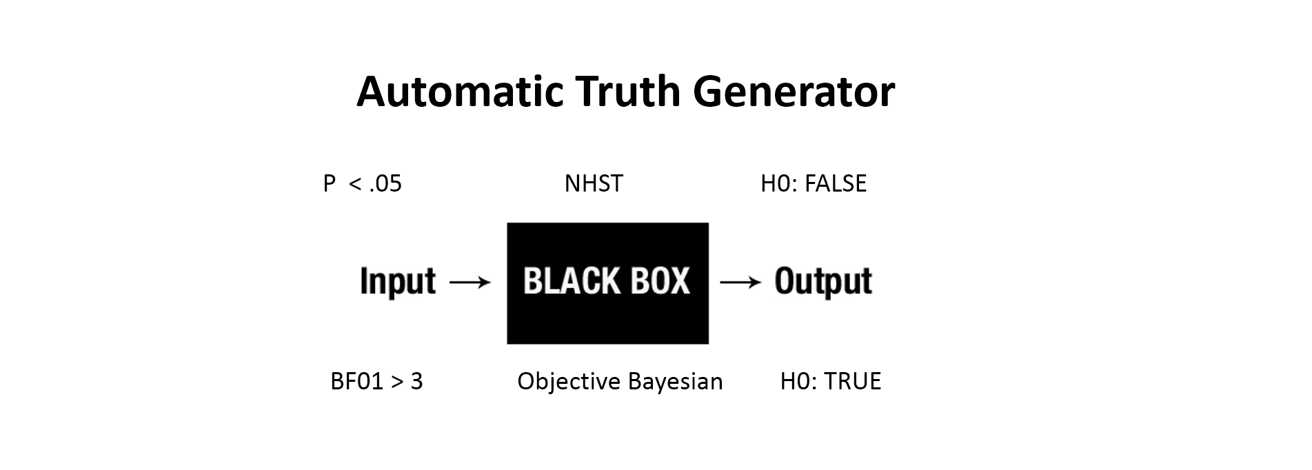
RMW suggest that the use of p-values is a fundamental problem that has contributed to the crisis of confidence and they offer Bayesian statistics as a solution to the problem.

In their own words, “the target of this critique is the practice of performing significance tests and reporting associated p-values”

This statement makes clear that the authors do not recognize selective reporting of p-values smaller than .05 as the problem, but rather question the usefulness of computing p-values in general.  In this way, they conflate an old and unresolved controversy amongst statisticians with the credibility crisis in psychology.

RMW point out that statisticians have been fighting over the right way to conduct inferential statistics for decades without any resolution.  One argument against p-values is that a significance criterion leads to a dichotomous decision when data can only strengthen or weaken the probability that a hypothesis is true or false.  That is, a p-value of .04 does not suddenly prove that a hypothesis is true.  It is just more likely that the hypothesis is true than if a study had produced a p-value of .20.  This point has been made in a classic article by Rozenboom that is cited by RMW.

“The null-hypothesis significance test treats ‘acceptance’ or ‘rejection’ of a hypothesis as though these were decisions one makes. But a hypothesis is not something, like a piece of pie offered for dessert, which can be accepted or rejected by a voluntary physical action. Acceptance or rejection of a hypothesis is a cognitive process, a degree of believing or disbelieving which, if rational, is not a matter of choice but determined solely by how likely it is, given the evidence, that the hypothesis is true.” (p. 422–423)

This argument ignores that decisions have to be made. Researchers have to decide whether they want to conduct follow-up studies, editors have to decide whether the evidence is sufficient to accept a manuscript for publication, and textbook writers have to decide whether they want to include an article in a textbook.  A type-I error probability of 5% has evolved as a norm for giving a researcher the benefit of the doubt that the hypothesis is true.  If this criterion were applied rigorously, no more than 5% of published results would be type-I errors.  Moreover, replication studies would quickly weed out false-positives because the chance of repeated type-I errors decreases quickly to zero if failed replication studies are reported.

Even if we agree that there is a problem with a decision criterion, it is not clear what a Bayesian science would look like.  Would newspaper articles report that a new studies increased the evidence for the effect of exercise on health from a 3:1 to a 10:1 ratio to being true? Would articles report Bayes-Factors without inferences that an effect exists?  It seems to defeat the purpose of an inferential statistical approach if the outcome of the inference process is not a conclusion that leads to a change in beliefs and even though beliefs can be true or false to varying degrees, beliefs are a black or white matter (I either believe that Berlin is the capital of Germany or not.

In fact, a review of articles that reported Bayes-Factors shows that most of these articles use Bayes-Factors to draw conclusions about hypotheses.  Currently, Bayes-Factors are mostly used to claim support for the absence of an effect when the Bayes-Factor favors the point-null hypothesis over an alternative hypothesis that predicted an effect.  This conclusion is typically made when the Bayes-Factor favors the null-hypothesis over the alternative hypothesis by a ratio of 3:1 or more.  RMW may disagree with this use of Bayes Factors, but this is how their statistical approach is currently being used. In essence, BF > 3 is used like p < .05.  It is easy to see how this change to Bayesian statistics does not solve the credibility crisis if only studies that produced Bayes-Factors greater than 3 are reported.  The only new problem is that authors may publish results that suggest effects do not exist at all, but that this conclusion is a classic type-II error (there is an effect, but the study had insufficient power to show the effect).

For example, Shanks et al. (2016) reported 30 statistical tests of the null-hypothesis and all tests favored the null-hypothesis over the alternative hypothesis and 29 tests exceeded the criterion of BF > 3.  Based on these results. Shanks et al. (2016) conclude that “as indicated by the Bayes factor analyses, their results strongly support the null hypothesis of no effect.”

RMW may argue that the current use of Bayes-Factors is improper and that better training in the use of Bayesian methods will solve this problem.  It is therefore interesting to examine RMW’s vision of proper use of Bayesian statistics.

RMW state that the key difference between conventional statistics with p-values and Bayesian statistics is subjectivity.

“Subjectivity is the key to principled measures of evidence for theory from data.”

“A fully Bayesian approach centers subjectivity as essential for principled analysis”

“The subjectivist perspective provides a principled approach to inference that is transparent, honest, and productive.”

Importantly, they also characterize their own approach as consistent with the call for subjectivity in inferential statistics.

“The Bayesian-subjective approach advocated here has been 250 years in the making”

However, it is not clear where RMW’s approach allows researchers to specify their subjective beliefs.  RMW have developed or used an approach that is often characterized as objective Bayesian.   “A major goal of statistics (indeed science) is to find a completely coherent objective Bayesian methodology for learning from data. This is exemplified by the attitudes of Jeffreys (1961)”  (Berger, 2006). That is, rather than developing models based on a theoretical understanding of a research question, a generic model is used to test a point null-hypothesis (d =0) against a vague alternative hypothesis that there is an effect (d ≠ 0).  In this way, the test is similar to the traditional comparison of the null-hypothesis and the alternative hypothesis in conventional statistics.  The only difference is that Bayesian statistics aims to quantify the relative support for these two hypothesis.  This would be easy if the alternative hypothesis were specified as a competing point prediction with a specified effect size.  For example, are the data more consistent with an effect size of d = 0 or d = .5?  Specifying a fixed value would make this comparison subjective if theories are not sufficiently specified to make such precise predictions.  Thus, the subjective beliefs of a researcher are needed to pick a fixed effect size that is being compared to the null-hypothesis.  However, RMW advocate a Bayesian approach that specifies the alternative hypothesis as a distribution that covers all possible effect sizes.  Clearly no subjectivity is needed to state an alternative hypothesis that the effect size can be anywhere between -∞ and +∞.

There is an infinite number of alternative hypothesis that can be constructed by assigning different weights to effect sizes for the infinite range of effect sizes.  These distributions can take on any form, although some may be more plausible than others.  Creating a plausible alternative hypothesis could involve subjective choices.  However, RMW’s advocate the use of a Cauchy distribution and their online tools and r-code only allow researchers to specify alternative hypotheses as a Cauchy distribution. Moreover, the Cauchy distribution is centered over zero, which implies that the most likely value for the alternative hypothesis is that there is no effect.  This violates the idea of subjectivity, because any researcher who tests a hypothesis against the null-hypothesis will assign the lowest probability to a zero value.  For example, if I think that the effect of exercise on weight loss is d = .5, I am saying that the most likely outcome if my hypothesis is correct is an effect size of d = .5, not an effect size of d = 0.  There is nothing inherently wrong with specifying the alternative hypothesis as a Cauchy distribution centered over 0, but it does seem wrong to present this specification as a subjective approach to hypothesis testing.

For example, let’s assume Bem (2011) wanted to use Bayesian statistic to test the hypothesis that individuals can foresee random future events.  A Cauchy distribution centered over 0 means that he thinks a null-result is the most likely outcome of the study, but this distribution does not represent his prior expectations.  Based on a meta-analysis and his experience as a researcher, he expected a small effect size of d = .2.  Thus, a subjective prior would be centered around a small effect size and Bem clearly did not expect a zero effect size or negative effect sizes (i.e., people can predict future events with less accuracy than random guessing).  RMW ignore that other Bayesian statisticians allow for priors that are not centered over 0 and they do not compare their approach to these alternative specifications of prior distributions.

RMW’s approach to Bayesian statistics leaves one opportunity for subjectivity to specify the prior distribution.  This parameter is the scaling parameter of the Cauchy distribution. The scaling parameter divides the density (the area under the curve) so that 50% of the distribution is in the tails.  RMW initially used a scaling parameter of 1 as a default setting.  This scaling parameter implies that there the prior distribution allocates a 50% chance to effect sizes in the range from -1 to 1 and a 50% probability to larger effect sizes.  Using the same default setting makes the approach fully objective or non-subjective because the same a priori distribution is used independent of subjective beliefs relevant to a particular research question.  Rouder and Morey later changed the default setting to a scaling parameter of .707, whereas Wagenmakers continues to use a scaling parameter of 1.

RMW suggest that the use of a default scaling parameter is not the most optimal use of their approach. “We do not recommend a single default model, but a collection of models that may be tuned by a single parameter, the scale of the distribution on effect size.”  Jeff Rouder also provided R-code that allows researchers to specify their own prior distributions and compute Bayes-Factors for a given observed effect size and sample size (the posted R-script is limited to within-subject/one-sample t-tests).

However, RMW do not provide practical guidelines how researchers should translate their subjective beliefs into a model with the corresponding scaling factor.  RMW give only very minimal recommendations. They suggest that a scaling factor greater than 1 is implausible because it would give too much weight to large effect sizes.  Remember, that even a scaling factor of 1 implies that there is a 50% chance that the absolute effect size is greater than 1 standard deviation.  They also suggest that setting the scaling factor to values smaller than .2 “makes the a priori distribution unnecessarily narrow because it does not give enough credence to effect sizes normally observed in well-executed behavioral-psychological experiments.”  This still leaves a range of scaling factors ranging from .2 to 1.  RMW do not provide further guidelines how researchers should set the scaling parameter. Instead they suggest that the default setting of .707 “is perfectly reasonable in most contexts.”  They do not explain why a value of .707 is perfectly reasonable and in what context this value is not reasonable.  Thus, they do not provide help in setting subjectively meaningful parameters, but rather imply that the default model can be used without thinking about the actual research question.

In my opinion, the use of a default setting is unsatisfactory because the choice of the scaling factor has an influence on the Bayes-Factor.  As noted by RMW, “there certainly is an effect of scale. The largest effect occurs for t = 0.” When the t-value is 0, the data provide maximal support for the null-hypothesis.  In RMW’s example, changing the scaling parameter from .2 to 1, increases the odds of the null-hypothesis being true from 5 to 1 to 10:1.  For gamblers who put real money on the line, the difference in winning $5 or $10 is a notable difference.  If I want to win $100, I have to risk losing $10 or $20 by placing bets with odds of 10:1 versus 5:1, and the difference of $10 can buy you two lattes at Starbucks or a hot dog at a ballgame.

What is a reasonable prior in between-subject designs?

Given the lack of guidance from RMW, I would like to make my own suggestion based on Cohen’s work on standardized effect sizes and the wealth of information about typical standardized effect sizes from meta-analyses.

One possibility is to create a prior distribution that matches the typical effect sizes observed in psychological research.  Cohen provides some helpful guidelines for researchers so that they could conduct power analyses.   He suggested that a moderate effect size is a difference of half a standard deviation (d = .5).  For other metrics, like correlation coefficients, a moderate effect size was r = .3.  Other useful information comes from Richard, Bond, and Stokes-Zoota’s meta-analysis of 100 years of social psychological research that produced a median effect size of r = .21 (d ~ .4).  The recent replication of 100 studies in social and cognitive psychology also yielded a median effect size of r = .2 (OSC, Science, 2016).

 

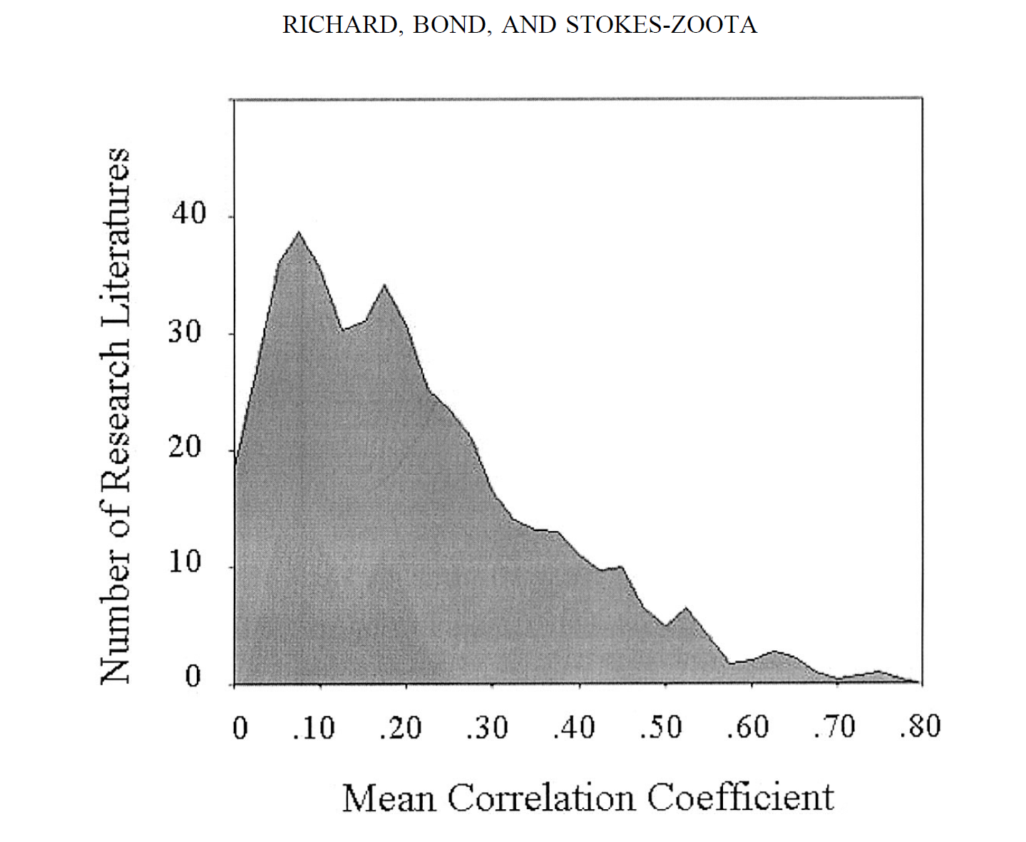
Figure of effect size distribution in Richard et al.

I suggest that researchers can translate their own subjective expectations into prior distributions by considering the distribution of effect sizes with the help of Cohen’s criteria for small, moderate, and large effect sizes.  That is, how many effect sizes does a researcher expect to be less than .2, between .2 and .5, between .5 and .8, and larger than .8?

A distribution that produces this expectation can be found using either a Cauchy or a Normal distribution and by changing the parameters for the mean and variability.

 

center = .5
width = .5

p = c()
p[1] = pnorm(-.8,-center,width)
p[2] = pnorm(-.5,-center,width) – pnorm(-.8,-center,width)
p[3] = pnorm(-.2,-center,width) – pnorm(-.5,-center,width)
p[4] = pnorm(0,-center,width) – pnorm(-.2,-center,width)
p = p / sum(p)
p

p = c()
p[1] = pcauchy(-.8,-center,width)
p[2] = pcauchy(-.5,-center,width) – pcauchy(-.8,-center,width)
p[3] = pcauchy(-.2,-center,width) – pcauchy(-.5,-center,width)
p[4] = pcauchy(0,-center,width) – pcauchy(-.2,-center,width)
p = p / sum(p)
p

The problem for the Cauchy distribution centered over 0 is that it is impossible to specify the assumption that effect sizes will fall into the small to large range (Table 1).   To create this scenario, RMW use a gamma distribution, but a gamma distribution has a step decline because it has to asymptote to 0 for an effect size of 0.  A normal distribution centered over a moderate effect size does not have this unrealistic property.  RMW also provide no subjective reason for the choice of a Cauchy distribution, which is not surprising because it originated in Jeffrey’s work that tried to create a fully objective Bayesian approach.

 

Cohen’s d	Cauchy(0,1)	Cauchy(0,.707)	Cauchy(0,.4)	Cauchy(0,.2)
.0 – .2	13	18	30	50
.2 – .5	17	22	28	26
.5 – .8	13	15	13	09
> .8	57	46	30	16

 

To obtain a priori distribution with higher probabilities for moderate effect sizes, it is necessary to shift the center of the distribution from 0 to a moderate effect size.  This can be done with a normal distribution or a Cauchy distribution.  However, Table 2 shows the the Cauchy distribution gives too much weight to large effect sizes. A normal distribution centered at d = .5 and a Standard deviation of .5 also gives too much weight to large effect sizes.

 

Cohen’s d	Norm(.5,.5)	Norm(.4,.4)	Cauchy(.5,.5)	Cauchy(.4,.4)
.0 – .2	14	18	10	14
.2 – .5	27	34	23	30
.5 – .8	27	29	23	23
> .8	33	19	44	33

 

In my opinion, a normal distribution with a mean of .4 and a standard deviation of .4 produces a reasonable prior distribution of effect sizes that matches the meta-analytic distribution of effect sizes reasonably well.  This prior distribution assigns a probability of 63% to effect sizes in the range between .2 and .8 and about equal probabilities to smaller and larger effect sizes.

The prior distribution is an important integral part of Bayesian inference.  Unlike p-values, Bayes-Factors can only be interpreted conditional on the prior distribution. A Bayes-Factor that favors the alternative over the point null-hypothesis can be used to bet on the presence of an effect, but it does not provide information about the size of the effect.  A Bayes-Factor that favors the null-hypothesis over an alternative only means that it is better to bet on the null-hypothesis than to bet on a specific weighted composite of effect sizes (e.g., a distributed bet with $1 on d = .2, $5 on d = .5, and $10 on d = .8). This bet may be a bad bet, but it may be better to bet $16 on d = .2 than to bet on d = .0.  To determine the odds for other bets, other priors would have to be tested.  Therefore, it is crucial that researchers who report Bayes-Factors as scientific information specify how they chose a prior distribution.  A Bayes-Factor in favor of the null-hypothesis with a Cauchy(0,10) that places a 50% probability on effect sizes of 10 standard deviations (e.g., an increase in IQ by 150 points) does not tell us that there is no effect. It only tells us that the researcher chose a bad prior.  Researchers can use the r-code provided by Jeff-Rouder or R-Code and online app provided by Dienes to compute Bayes-Factors for non-centered, normal priors.

CONCLUSIONS

In conclusion, RMW start their article with the credibility crisis in psychology, discuss Bayesian statistics as a solution, and suggest Jeffrey’s objective Bayesian approach as an alternative to traditional significance testing.  In my opinion, replacing significance testing with an objective Bayesian approach creates new problems that have not been solved and fails to address the root cause of the credibility crisis in psychology, namely the common practice of reporting only results that support a hypothesis that predicts an effect.  Therefore, I suggest that psychologists need to focus on open science and encourage full disclosure of data and research methods to fix the credibility problem.  Whether data are reported with p-values or Bayes-Factors, confidence intervals or credibility intervals is less important.  All articles should report basic statistics like means, unstandardized regression coefficients, standard deviations, and sampling error.  With this information, researchers can compute p-values, confidence intervals, or Bayes-Factors and draw their own conclusions from the data. Even better if the actual data are made available.  Good data will often survive bad statistical analysis (robustness), but good statistics cannot solve the problem of bad data.