Tag Archives: Replication

2021 Replicability Report for the Psychology Department at New York University

February 2, 2022UncategorizedPublication Bias, Questionable Research Practices, r-index, replicability, Replication, Social PsychologyUlrich Schimmack

Introduction

Since 2011, it is an open secret that many published results in psychology journals do not replicate. The replicability of published results is particularly low in social psychology (Open Science Collaboration, 2015).

A key reason for low replicability is that researchers are rewarded for publishing as many articles as possible without concerns about the replicability of the published findings. This incentive structure is maintained by journal editors, review panels of granting agencies, and hiring and promotion committees at universities.

To change the incentive structure, I developed the Replicability Index, a blog that critically examined the replicability, credibility, and integrity of psychological science. In 2016, I created the first replicability rankings of psychology departments (Schimmack, 2016). Based on scientific criticisms of these methods, I have improved the selection process of articles to be used in departmental reviews.

1. I am using Web of Science to obtain lists of published articles from individual authors (Schimmack, 2022). This method minimizes the chance that articles that do not belong to an author are included in a replicability analysis. It also allows me to classify researchers into areas based on the frequency of publications in specialized journals. Currently, I cannot evaluate neuroscience research. So, the rankings are limited to cognitive, social, developmental, clinical, and applied psychologists.

2. I am using department’s websites to identify researchers that belong to the psychology department. This eliminates articles that are from other departments.

3. I am only using tenured, active professors. This eliminates emeritus professors from the evaluation of departments. I am not including assistant professors because the published results might negatively impact their chances to get tenure. Another reason is that they often do not have enough publications at their current university to produce meaningful results.

Like all empirical research, the present results rely on a number of assumptions and have some limitations. The main limitations are that
(a) only results that were found in an automatic search are included
(b) only results published in 120 journals are included (see list of journals)
(c) published significant results (p < .05) may not be a representative sample of all significant results
(d) point estimates are imprecise and can vary based on sampling error alone.

These limitations do not invalidate the results. Large difference in replicability estimates are likely to predict real differences in success rates of actual replication studies (Schimmack, 2022).

New York University

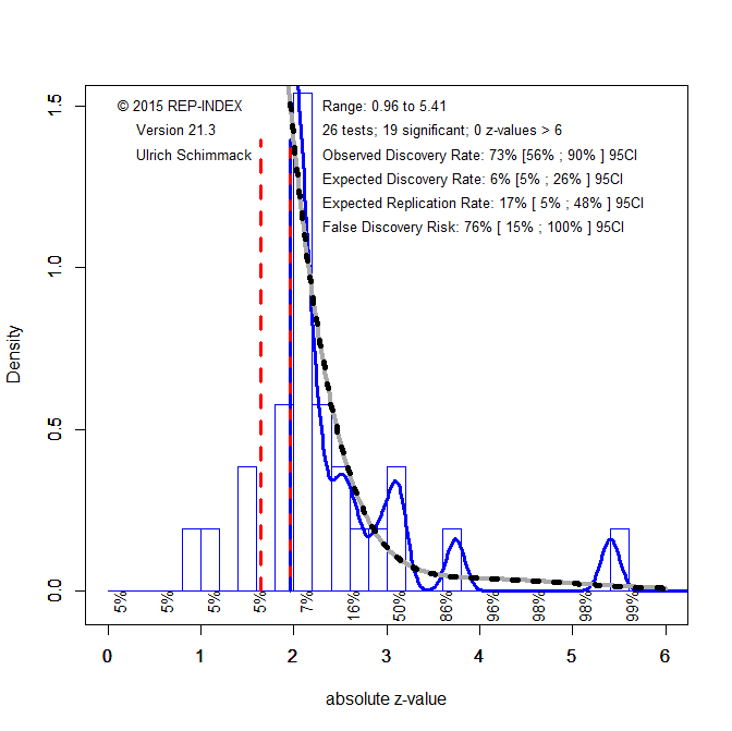
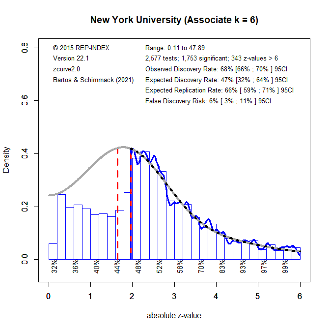
I used the department website to find core members of the psychology department. I found 13 professors and 6 associate professors. Figure 1 shows the z-curve for all 12,365 tests statistics in articles published by these 19 faculty members. I use the Figure to explain how a z-curve analysis provides information about replicability and other useful meta-statistics.

1. All test-statistics are converted into absolute z-scores as a common metric of the strength of evidence (effect size over sampling error) against the null-hypothesis (typically H0 = no effect). A z-curve plot is a histogram of absolute z-scores in the range from 0 to 6. The 1,239 (~ 10%) of z-scores greater than 6 are not shown because z-scores of this magnitude are extremely unlikely to occur when the null-hypothesis is true (particle physics uses z > 5 for significance). Although they are not shown, they are included in the meta-statistics.

2. Visual inspection of the histogram shows a steep drop in frequencies at z = 1.96 (dashed blue/red line) that corresponds to the standard criterion for statistical significance, p = .05 (two-tailed). This shows that published results are selected for significance. The dashed red/white line shows significance for p < .10, which is often used for marginal significance. There is another drop around this level of significance.

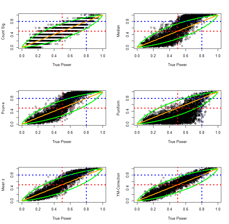
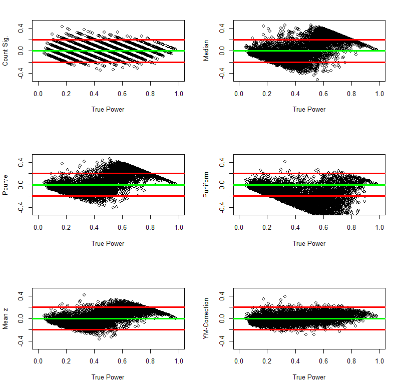
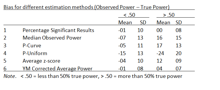
3. To quantify the amount of selection bias, z-curve fits a statistical model to the distribution of statistically significant results (z > 1.96). The grey curve shows the predicted values for the observed significant results and the unobserved non-significant results. The full grey curve is not shown to present a clear picture of the observed distribution. The statistically significant results (including z > 6) make up 20% of the total area under the grey curve. This is called the expected discovery rate because the results provide an estimate of the percentage of significant results that researchers actually obtain in their statistical analyses. In comparison, the percentage of significant results (including z > 6) includes 70% of the published results. This percentage is called the observed discovery rate, which is the rate of significant results in published journal articles. The difference between a 70% ODR and a 20% EDR provides an estimate of the extent of selection for significance. The difference of 50 percentage points is large. The upper level of the 95% confidence interval for the EDR is 28%. Thus, the discrepancy is not just random. To put this result in context, it is possible to compare it to the average for 120 psychology journals in 2010 (Schimmack, 2022). The ODR is similar (70 vs. 72%), but the EDR is a bit lower (20% vs. 28%), although the difference might be largely due to chance.

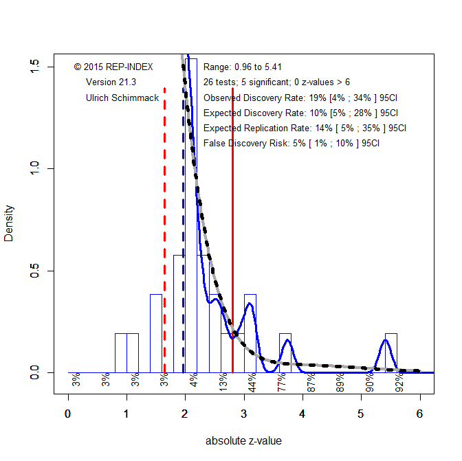
4. The EDR can be used to estimate the risk that published results are false positives (i.e., a statistically significant result when H0 is true), using Soric’s (1989) formula for the maximum false discovery rate. An EDR of 20% implies that no more than 20% of the significant results are false positives, however the upper limit of the 95%CI of the EDR, 28%, allows for 36% false positive results. Most readers are likely to agree that this is an unacceptably high risk that published results are false positives. One solution to this problem is to lower the conventional criterion for statistical significance (Benjamin et al., 2017). Figure 2 shows that alpha = .005 reduces the point estimate of the FDR to 3% with an upper limit of the 95% confidence interval of XX%. Thus, without any further information readers could use this criterion to interpret results published by NYU faculty members.

5. The estimated replication rate is based on the mean power of significant studies (Brunner & Schimmack, 2020). Under ideal condition, mean power is a predictor of the success rate in exact replication studies with the same sample sizes as the original studies. However, as NYU professor van Bavel pointed out in an article, replication studies are never exact, especially in social psychology (van Bavel et al., 2016). This implies that actual replication studies have a lower probability of producing a significant result, especially if selection for significance is large. In the worst case scenario, replication studies are not more powerful than original studies before selection for significance. Thus, the EDR provides an estimate of the worst possible success rate in actual replication studies. In the absence of further information, I have proposed to use the average of the EDR and ERR as a predictor of actual replication outcomes. With an ERR of 62% and an EDR of 20%, this implies an actual replication prediction of 41%. This is close to the actual replication rate in the Open Science Reproducibility Project (Open Science Collaboration, 2015). The prediction for results published in 120 journals in 2010 was (ERR = 67% + ERR = 28%)/ 2 = 48%. This suggests that results published by NYU faculty are slightly less replicable than the average result published in psychology journals, but the difference is relatively small and might be mostly due to chance.

6. There are two reasons for low replication rates in psychology. One possibility is that psychologists test many false hypotheses (i.e., H0 is true) and many false positive results are published. False positive results have a very low chance of replicating in actual replication studies (i.e. 5% when .05 is used to reject H0), and will lower the rate of actual replications a lot. Alternative, it is possible that psychologists tests true hypotheses (H0 is false), but with low statistical power (Cohen, 1961). It is difficult to distinguish between these two explanations because the actual rate of false positive results is unknown. However, it is possible to estimate the typical power of true hypotheses tests using Soric’s FDR. If 20% of the significant results are false positives, the power of the 80% true positives has to be (.62 – .2*.05)/.8 = 76%. This would be close to Cohen’s recommended level of 80%, but with a high level of false positive results. Alternatively, the null-hypothesis may never be really true. In this case, the ERR is an estimate of the average power to get a significant result for a true hypothesis. Thus, power is estimated to be between 62% and 76%. The main problem is that this is an average and that many studies have less power. This can be seen in Figure 1 by examining the local power estimates for different levels of z-scores. For z-scores between 2 and 2.5, the ERR is only 47%. Thus, many studies are underpowered and have a low probability of a successful replication with the same sample size even if they showed a true effect.

Area

The results in Figure 1 provide highly aggregated information about replicability of research published by NYU faculty. The following analyses examine potential moderators. First, I examined social and cognitive research. Other areas were too small to be analyzed individually.

The z-curve for the 11 social psychologists was similar to the z-curve in Figure 1 because they provided more test statistics and had a stronger influence on the overall result.

The z-curve for the 6 cognitive psychologists looks different. The EDR and ERR are higher for cognitive psychology, and the 95%CI for social and cognitive psychology do not overlap. This suggests systematic differences between the two fields. These results are consistent with other comparisons of the two fields, including actual replication outcomes (OSC, 2015). With an EDR of 44%, the false discovery risk for cognitive psychology is only 7% with an upper limit of the 95%CI at 12%. This suggests that the conventional criterion of .05 does keep the false positive risk at a reasonably low level or that an adjustment to alpha = .01 is sufficient. In sum, the results show that results published by cognitive researchers at NYU are more replicable than those published by social psychologists.

Position

Since 2015 research practices in some areas of psychology, especially social psychology, have changed to increase replicability. This would imply that research by younger researchers is more replicable than research by more senior researchers that have more publications before 2015. A generation effect would also imply that a department’s replicability increases when older faculty members retire. On the other hand, associate professors are relatively young and likely to influence the reputation of a department for a long time.

The figure above shows that most test statistics come from the (k = 13) professors. As a result, the z-curve looks similar to the z-curve for all test values in Figure 1. The results for the 6 associate professors (below) are more interesting. Although five of the six associate professors are in the social area, the z-curve results show a higher EDR and less selection bias than the plot for all social psychologists. This suggests that the department will improve when full professors in social psychology retire.

Some researchers have changed research practices in response to the replication crisis. It is therefore interesting to examine whether replicability of newer research has improved. To examine this question, I performed a z-curve analysis for articles published in the past five year (2016-2021).

The results show very little signs of improvement. The EDR increased from 20% to 26%, but the confidence intervals are too wide to infer that this is a systematic change. In contrast, Stanford University improved from 22% to 50%, a significant increase. For now, NYU results should be interpreted with alpha = .005 as threshold for significance to maintain a reasonable false positive risk.

The table below shows the meta-statistics of all 19 faculty members. You can see the z-curve for each faculty member by clicking on their name.

Rank	Name	ARP	EDR	ERR	FDR
1	Karen E. Adolph	66	76	56	4
2	Bob Rehder	61	75	47	6
3	Marjorie Rhodes	58	68	48	6
4	Jay J. van Bavel	55	66	44	7
5	Brian McElree	54	59	49	6
6	David M. Amodio	53	65	40	8
7	Todd M. Gureckis	49	75	23	17
8	Emily Balcetis	48	68	28	13
9	Eric D. Knowles	48	60	35	10
10	Tessa V. West	46	55	37	9
11	Catherine A. Hartley	45	70	19	23
12	Madeline E. Heilman	44	66	23	18
13	John T. Jost	44	62	26	15
14	Andrei Cimpian	42	64	20	21
15	Peter M. Gollwitzer	36	54	18	25
16	Yaacov Trope	34	54	14	32
17	Gabriele Oettingen	30	46	14	32
18	Susan M. Andersen	30	47	13	35

Incidental Anchoring Bites the Dust

June 4, 2021UncategorizedAnchoring, Incidental Anchoring, Kahneman, Kahneman & Tversky 1974, Meta-Analysis, Publication Bias, Replication, TverskyUlrich Schimmack

Update: 6/10/21

After I posted this post, I learned about a published meta-analysis and new studies of incidental anchoring by David Shanks and colleagues that came to the same conclusion (Shanks et al., 2020).

Introduction

“The most expensive car in the world costs $5 million. How much does a new BMW 530i cost?”

According to anchoring theory, information about the most expensive car can lead to higher estimates for the cost of a BMW. Anchoring effects have been demonstrated in many credible studies since the 1970s (Kahneman & Tversky, 1973).

A more controversial claim is that anchoring effects even occur when the numbers are unrelated to the question and presented incidentally (Criticher & Gilovich, 2008). In one study, participants saw a picture of a football player and were asked to guess how likely it is that the player will sack the football player in the next game. The player’s number on jersey was manipulated to be 54 or 94. The study produced a statistically significant result suggesting that a higher number makes people give higher likelihood judgments. This study started a small literature on incidental anchoring effects. A variation on this them are studies that presented numbers so briefly on a computer screen that most participants did not actually see the numbers. This is called subliminal priming. Allegedly, subliminal priming also produced anchoring effects (Mussweiler & Englich (2005).

Since 2011, many psychologists are skeptical whether statistically significant results in published articles can be trusted. The reason is that researchers only published results that supported their theoretical claims even when the claims were outlandish. For example, significant results also suggested that extraverts can foresee where pornographic images are displayed on a computer screen even before the computer randomly selected the location (Bem, 2011). No psychologist, except Bem, believes these findings. More problematic is that many other findings are equally incredible. A replication project found that only 25% of results in social psychology could be replicated (Open Science Collaboration, 2005). So, the question is whether incidental and subliminal anchoring are more like classic anchoring or more like extrasensory perception.

There are two ways to assess the credibility of published results when publication bias is present. One approach is to conduct credible replication studies that are published independent of the outcome of a study. The other approach is to conduct a meta-analysis of the published literature that corrects for publication bias. A recent article used both methods to examine whether incidental anchoring is a credible effect (Kvarven et al., 2020). In this article, the two approaches produced inconsistent results. The replication study produced a non-significant result with a tiny effect size, d = .04 (Klein et al., 2014). However, even with bias-correction, the meta-analysis suggested a significant, small to moderate effect size, d = .40.

Results

The data for the meta-analysis were obtained from an unpublished thesis (Henriksson, 2015). I suspected that the meta-analysis might have coded some studies incorrectly. Therefore, I conducted a new meta-analysis, using the same studies and one new study. The main difference between the two meta-analysis is that I coded studies based on the focal hypothesis test that was used to claim evidence for incidental anchoring. The p-values were then transformed into fisher-z transformed correlations and and sampling error, 1/sqrt(N – 3), based on the sample sizes of the studies.

Whereas the old meta-analysis suggested that there is no publication bias, the new meta-analysis showed a clear relationship between sampling error and effect sizes, b = 1.68, se = .56, z = 2.99, p = .003. Correcting for publication bias produced a non-significant intercept, b = .039, se = .058, z = 0.672, p = .502, suggesting that the real effect size is close to zero.

Figure 1 shows the regression line for this model in blue and the results from the replication study in green. We see that the blue and green lines intersect when sampling error is close to zero. As sampling error increases because sample sizes are smaller, the blue and green line diverge more and more. This shows that effect sizes in small samples are inflated by selection for significance.

However, there is some statistically significant variability in the effect sizes, I2 = 36.60%, p = .035. To further examine this heterogeneity, I conducted a z-curve analysis (Bartos & Schimmack, 2021; Brunner & Schimmack, 2020). A z-curve analysis converts p-values into z-statistics. The histogram of these z-statistics shows publication bias, when z-statistics cluster just above the significance criterion, z = 1.96.

Figure 2 shows a big pile of just significant results. As a result, the z-curve model predicts a large number of non-significant results that are absent. While the published articles have a 73% success rate, the observed discovery rate, the model estimates that the expected discovery rate is only 6%. That is, for every 100 tests of incidental anchoring, only 6 studies are expected to produce a significant result. To put this estimate in context, with alpha = .05, 5 studies are expected to be significant based on chance alone. The 95% confidence interval around this estimate includes 5% and is limited at 26% at the upper end. Thus, researchers who reported significant results did so based on studies with very low power and they needed luck or questionable research practices to get significant results.

A low discovery rate implies a high false positive risk. With an expected discovery rate of 6%, the false discovery risk is 76%. This is unacceptable. To reduce the false discovery risk, it is possible to lower the alpha criterion for significance. In this case, lowering alpha to .005 produces a false discovery risk of 5%. This leaves 5 studies that are significant.

One notable study with strong evidence, z = 3.70, examined anchoring effects for actual car sales. The data came from an actual auction of classic cars. The incidental anchors were the prices of the previous bid for a different vintage car. Based on sales data of 1,477 cars, the authors found a significant effect, b = .15, se = .04 that translates into a standardized effect size of d = .2 (fz = .087). Thus, while this study provides some evidence for incidental anchoring effects in one context, the effect size estimate is also consistent with the broader meta-analysis that effect sizes of incidental anchors are fairly small. Moreover, the incidental anchor in this study is still in the focus of attention and in some way related to the actual bid. Thus, weaker effects can be expected for anchors that are not related to the question at all (a player’s number) or anchors presented outside of awareness.

Conclusion

There is clear evidence that evidence for incidental anchoring cannot be trusted at face value. Consistent with research practices in general, studies on incidental and subliminal anchoring suffer from publication bias that undermines the credibility of the published results. Unbiased replication studies and meta-analysis suggest that incidental anchoring effects are either very small or zero. Thus, there exists currently no empirical support for the notion that irrelevant numeric information can bias numeric judgments. More research on anchoring effects that corrects for publication bias is needed.

Replicability Audit of John A. Bargh

March 17, 2019Bargh, Priming, Questionable Research Practices, Replicability, Replicability Audit, Replication CrisisBargh, Doyen, Questionable Research Practices, replicability, Replication, Replication CrisisUlrich Schimmack

“Trust is good, but control is better”

INTRODUCTION

Information about the replicability of published results is important because empirical results can only be used as evidence if the results can be replicated. However, the replicability of published results in social psychology is doubtful. Brunner and Schimmack (2020) developed a statistical method called z-curve to estimate how replicable a set of significant results are, if the studies were replicated exactly. In a replicability audit, I am applying z-curve to the most cited articles of psychologists to estimate the replicability of their studies.

John A. Bargh

Bargh is an eminent social psychologist (H-Index in WebofScience = 61). He is best known for his claim that unconscious processes have a strong influence on behavior. Some of his most cited article used subliminal or unobtrusive priming to provide evidence for this claim.

Bargh also played a significant role in the replication crisis in psychology. In 2012, a group of researchers failed to replicate his famous “elderly priming” study (Doyen et al., 2012). He responded with a personal attack that was covered in various news reports (Bartlett, 2013). It also triggered a response by psychologist and Nobel Laureate Daniel Kahneman, who wrote an open letter to Bargh (Young, 2012).

“As all of you know, of course, questions have been raised about the robustness of priming results…. your field is now the poster child for doubts about the integrity of psychological research.”

Kahneman also asked Bargh and other social priming researchers to conduct credible replication studies to demonstrate that the effects are real. However, seven years later neither Bargh nor other prominent social priming researchers have presented new evidence that their old findings can be replicated.

Instead other researchers have conducted replication studies and produced further replication failures. As a result, confidence in social priming is decreasing – but not as fast as it should gifen replication failures and lack of credibility – as reflected in Bargh’s citation counts (Figure 1)

Figure 1. John A. Bargh’s citation counts in Web of Science (updated 9/29/23)

In this blog post, I examine the replicability and credibility of John A. Bargh’s published results using z-curve. It is well known that psychology journals only published confirmatory evidence with statistically significant results, p < .05 (Sterling, 1959). This selection for significance is the main cause of the replication crisis in psychology because selection for significance makes it impossible to distinguish results that can be replicated from results that cannot be replicated because selection for significance ensures that all results will be replicated (we never see replication failures).

While selection for significance makes success rates uninformative, the strength of evidence against the null-hypothesis (signal/noise or effect size / sampling error) does provide information about replicability. Studies with higher signal to noise ratios are more likely to replicate. Z-curve uses z-scores as the common metric of signal-to-noise ratio for studies that used different test statistics. The distribution of observed z-scores provides valuable information about the replicability of a set of studies. If most z-scores are close to the criterion for statistical significance (z = 1.96), replicability is low.

Given the requirement to publish significant results, researches had two options how they could meet this goal. One option requires obtaining large samples to reduce sampling error and therewith increase the signal-to-noise ratio. The other solution is to conduct studies with small samples and conduct multiple statistical tests. Multiple testing increases the probability of obtaining a significant results with the help of chance. This strategy is more efficient in producing significant results, but these results are less replicable because a replication study will not be able to capitalize on chance again. The latter strategy is called a questionable research practice (John et al., 2012), and it produces questionable results because it is unknown how much chance contributed to the observed significant result. Z-curve reveals how much a researcher relied on questionable research practices to produce significant results.

Data

I used WebofScience to identify the most cited articles by John A. Bargh (datafile). I then selected empirical articles until the number of coded articles matched the number of citations, resulting in 43 empirical articles (H-Index = 41). The 43 articles reported 111 studies (average 2.6 studies per article). The total number of participants was 7,810 with a median of 56 participants per study. For each study, I identified the most focal hypothesis test (MFHT). The result of the test was converted into an exact p-value and the p-value was then converted into a z-score. The z-scores were submitted to a z-curve analysis to estimate mean power of the 100 results that were significant at p < .05 (two-tailed). Four studies did not produce a significant result. The remaining 7 results were interpreted as evidence with lower standards of significance. Thus, the success rate for 111 reported hypothesis tests was 96%. This is a typical finding in psychology journals (Sterling, 1959).

Results

The z-curve estimate of replicability is 29% with a 95%CI ranging from 15% to 38%. Even at the upper end of the 95% confidence interval this is a low estimate. The average replicability is lower than for social psychology articles in general (44%, Schimmack, 2018) and for other social psychologists. At present, only one audit has produced an even lower estimate (Replicability Audits, 2019).

The histogram of z-values shows the distribution of observed z-scores (blue line) and the predicted density distribution (grey line). The predicted density distribution is also projected into the range of non-significant results. The area under the grey curve is an estimate of the file drawer of studies that need to be conducted to achieve 100% successes if hiding replication failures were the only questionable research practice that is used. The ratio of the area of non-significant results to the area of all significant results (including z-scores greater than 6) is called the File Drawer Ratio. Although this is just a projection, and other questionable practices may have been used, the file drawer ratio of 7.53 suggests that for every published significant result about 7 studies with non-significant results remained unpublished. Moreover, often the null-hypothesis may be false, but the effect size is very small and the result is still difficult to replicate. When the definition of a false positive includes studies with very low power, the false positive estimate increases to 50%. Thus, about half of the published studies are expected to produce replication failures.

Finally, z-curve examines heterogeneity in replicability. Studies with p-values close to .05 are less likely to replicate than studies with p-values less than .0001. This fact is reflected in the replicability estimates for segments of studies that are provided below the x-axis. Without selection for significance, z-scores of 1.96 correspond to 50% replicability. However, we see that selection for significance lowers this value to just 14% replicability. Thus, we would not expect that published results with p-values that are just significant would replicate in actual replication studies. Even z-scores in the range from 3 to 3.5 average only 32% replicability. Thus, only studies with z-scores greater than 3.5 can be considered to provide some empirical evidence for this claim.

Inspection of the datafile shows that z-scores greater than 3.5 were consistently obtained in 2 out of the 43 articles. Both articles used a more powerful within-subject design.

The automatic evaluation effect: Unconditional automatic attitude activation with a pronunciation task (JPSP, 1996)

Subjective aspects of cognitive control at different stages of processing (Attention, Perception, & Psychophysics, 2009).

Conclusion

John A. Bargh’s work on unconscious processes with unobtrusive priming task is at the center of the replication crisis in psychology. This replicability audit suggests that this is not an accident. The low replicability estimate and the large file-drawer estimate suggest that replication failures are to be expected. As a result, published results cannot be interpreted as evidence for these effects.

So far, John Bargh has ignored criticism of his work. In 2017, he published a popular book about his work on unconscious processes. The book did not mention doubts about the reported evidence, while a z-curve analysis showed low replicability of the cited studies (Schimmack, 2017).

Recently, another study by John Bargh failed to replicate (Chabris et al., in press), and Jessy Singal wrote a blog post about this replication failure (Research Digest) and John Bargh wrote a lengthy comment.

In the commentary, Bargh lists several studies that successfully replicated the effect. However, listing studies with significant results does not provide evidence for an effect unless we know how many studies failed to demonstrate the effect and often we do not know this because these studies are not published. Thus, Bargh continues to ignore the pervasive influence of publication bias.

Bargh then suggests that the replication failure was caused by a hidden moderator which invalidates the results of the replication study.

One potentially important difference in procedure is the temperature of the hot cup of coffee that participants held: was the coffee piping hot (so that it was somewhat uncomfortable to hold) or warm (so that it was pleasant to hold)? If the coffee was piping hot, then, according to the theory that motivated W&B, it should not activate the concept of social warmth – a positively valenced, pleasant concept. (“Hot” is not the same as just more “warm”, and actually participates in a quite different metaphor – hot vs. cool – having to do with emotionality.) If anything, an uncomfortably hot cup of coffee might be expected to activate the concept of anger (“hot-headedness”), which is antithetical to social warmth. With this in mind, there are good reasons to suspect that in C&S, the coffee was, for many participants, uncomfortably hot. Indeed, C&S purchased a hot or cold coffee at a coffee shop and then immediately handed that coffee to passersby who volunteered to take the study. Thus, the first few people to hold a hot coffee likely held a piping hot coffee (in contrast, W&B’s coffee shop was several blocks away from the site of the experiment, and they used a microwave for subsequent participants to keep the coffee at a pleasantly warm temperature). Importantly, C&S handed the same cup of coffee to as many as 7 participants before purchasing a new cup. Because of that feature of their procedure, we can check if the physical-to-social warmth effect emerged after the cups were held by the first few participants, at which point the hot coffee (presumably) had gone from piping hot to warm.

He overlooks that his original study produced only weak evidence for the effect with a p-value of .0503, that is technically not below the .05 value for significance. As shown in the z-curve plot, results with a p-value of .0503 have only an average replicability of 13%. Moreover, the 95%CI for the effect size touches 0. Thus, the original study did not rule out that the effect size is extremely small and has no practical significance. To make any claims that the effect of holding a warm cup on affection is theoretically relevant for our understanding of affection would require studies with larger samples and more convincing evidence.

At the end of his commentary, John A. Bargh assures readers that he is purely motivated by a search for the truth.

Let me close by affirming that I share your goal of presenting the public with accurate information as to the state of the scientific evidence on any finding I discuss publicly. I also in good faith seek to give my best advice to the public at all times, again based on the present state of evidence. Your and my assessments of that evidence might differ, but our motivations are the same.

Let me be crystal clear. I have no reasons to doubt that John A. Bargh believes what he says. His conscious mind sees himself as a scientist who employs the scientific method to provide objective evidence. However, Bargh himself would be the first to acknowledge that our conscious mind is not fully aware of the actual causes of human behavior. I submit that his response to criticism of his work shows that he is less capable of being objective than he thinks he his. I would be happy to be proven wrong in a response by John A. Bargh to my scientific criticism of his work. So far, eminent social psychologists have preferred to remain silent about the results of their replicability audits.

Disclaimer

It is nearly certain that I made some mistakes in the coding of John A. Bargh’s articles. However, it is important to distinguish consequential and inconsequential mistakes. I am confident that I did not make consequential errors that would alter the main conclusions of this audit. However, control is better than trust and everybody can audit this audit. The data are openly available and the data can be submitted to a z-curve analysis using a shinny app. Thus, this replicability audit is fully transparent and open to revision.

Postscript

Many psychologists do not take this work seriously because it has not been peer-reviewed. However, nothing is stopping them from conducting a peer-review of this work and to publish the results of their review as a commentary here or elsewhere. Thus, the lack of peer-review is not a reflection of the quality of this work, but rather a reflection of the unwillingness of social psychologists to take criticism of their work seriously.

If you found this audit interesting, you might also be interested in other replicability audits of eminent social psychologists.

Thinking Too Fast About Life-Satisfaction Judgments

November 27, 2018Fritz Strack, Item_Order Effects, Kahneman, Life-Satisfaction, Norbert Schwarz, Satisfaction with Life ScaleItem-Order Effects, Kahneman, Life-Satisfaction, Meta-Analysis, Publication Bias, Replication, Schwarz, Strack, Thinking Fast and SlowUlrich Schimmack

In 2002, Daniel Kahneman was awarded the Nobel Prize for Economics. He received the award for his groundbreaking work on human irrationality in collaboration with Amos Tversky in the 1970s.

In 1999, Daniel Kahneman was the lead editor of the book “Well-Being: The foundations of Hedonic Psychology.” Subsequently, Daniel Kahneman conducted several influential studies on well-being.

The aim of the book was to draw attention to hedonic or affective experiences as an important, if not the sole, contributor to human happiness. He called for a return to Bentham’s definition of a good life as a life filled with pleasure and devoid of pain a.k.a displeasure.

The book was co-edited by Norbert Schwarz and Ed Diener, who both contributed chapters to the book. These chapters make contradictory claims about the usefulness of life-satisfaction judgments as an alternative measure of a good life.

Ed Diener is famous for his conception of wellbeing in terms of a positive hedonic balance (lot’s of pleasure, little pain) and high life-satisfaction. In contrast, Schwarz is known as a critic of life-satisfaction judgments. In fact, Schwarz and Strack’s contribution to the book ended with the claim that “most readers have probably concluded that there is little to be learned from self-reports of global well-being” (p. 80).

To a large part, Schwarz and Strack’s pessimistic view is based on their own studies that seemed to show that life-satisfaction judgments are influenced by transient factors such as current mood or priming effects.

“the obtained reports of SWB are subject to pronounced question-order- effects because the content of preceding questions influences the temporary accessibility of relevant information” (Schwarz & Strack, p. 79).

There is only one problem with this claim; it is only true for a few studies conducted by Schwarz and Strack. Studies by other researchers have produced much weaker and often not statistically reliable context effects (see Schimmack & Oishi, 2005, for a meta-analysis).
In fact, a recent attempt to replicate Schwarz and Strack’s results in a large sample of over 7,000 participants failed to show the effect and even found a small, but statistically significant effect in the opposite direction (ManyLabs2).

Figure 1 summarizes the results of the meta-analysis from Schimmack and Oishi 2005), but it is enhanced by new developments in meta-analysis. The blue line in the graph regresses effect sizes (converted into Fisher-z scores) onto sampling error (1/sqrt(N -3). Publication bias and other statistical tricks produce a correlation between effect size and sampling error. The slope of the blue line shows clear evidence of publication bias, z = 3.85, p = .0001. The intercept (where the line meets zero on the x-axis) can be interpreted as a bias-corrected estimate of the real effect size. The value is close to zero and not statistically significant, z = 1.70, p = .088. The green line shows the effect size in the replication study, which was also close to zero, but statistically significant in the opposite direction. The orange vertical red line shows the average effect size without controlling for publication bias. We see that this naive meta-analysis overestimates the effect size and falsely suggests that item-order effects are a robust phenomenon. Finally, the graph highlights the three results from studies by Strack and Schwarz. These results are clear outliers and even above the biased blue regression line. The biggest outlier was obtained by Strack et al. (1991) and this is the finding that is featured in Kahneman’s book, even though it is not reproducible and clearly inflated by sampling error. Interestingly, sampling error is also called noise and Kahneman wrote a whole new book about the problems of noise in human judgments.

While the figure is new, the findings were published in 2005, several years before Kahneman wrote his book “Thinking Fast and Slow). He was simply to lazy to use the slow process of a thorough literature research to write about life-satisfaction judgments. Instead, he relied on a fast memory search that retrieved a study by his buddy. Thus, while the chapter is a good example of biases that result from fast information processing, it is not a good chapter to tell readers about life-satisfaction judgments.

To be fair, Kahneman did inform his readers that he is biased against life-satisfaction judgments. Having come to the topic of well-being from the study of the mistaken memories of colonoscopies and painfully cold hands, I was naturally suspicious of global satisfaction with life as a valid measure of well-being (Kindle Locations 6796-6798). Later on, he even admits to his mistake. Life satisfaction is not a flawed measure of their experienced well-being, as I thought some years ago. It is something else entirely (Kindle Location 6911-6912).

However, insight into his bias was not enough to motivate him to search for evidence that may contradict his bias. This is known as confirmation bias. Even ideal-prototypes of scientists like Nobel Laureates are not immune to this fallacy. Thus, this example shows that we cannot rely on simple cues like “professor at Ivy League,” “respected scientists,” or “published in prestigious journals.” to trust scientific claims. Scientific claims need to be backed up by credible evidence. Unfortunately, social psychology has produced a literature that is not trustworthy because studies were only published if they confirmed theories. It will take time to correct these mistakes of the past by carefully controlling for publication bias in meta-analyses and by conducting pre-registered studies that are published even if they falsify theoretical predictions. Until then, readers should be skeptical about claims based on psychological ‘science,’ even if they are made by a Nobel Laureate.

When Exact Replications Are Too Exact: The Lucky-Bounce-Test for Pairs of Exact Replication Studies

May 27, 2015Power, science, StatisticsBargh, Elderly Stereotype, Exact Replication, Meta-Analysis, Post-Hoc-Power, Power, Priming, Publication Bias, Questionable Research Practices, ReplicationUlrich Schimmack

Imagine an NBA player has an 80% chance to make one free throw. What is the chance that he makes both free throws? The correct answer is 64% (80% * 80%).

Now consider the possibility that it is possible to distinguish between two types of free throws. Some free throws are good; they don’t touch the rim and make a swishing sound when they go through the net (all net). The other free throws bounce of the rim and go in (rattling in).

What is the probability that an NBA player with an 80% free throw percentage makes a free throw that is all net or rattles in? It is more likely that an NBA player with an 80% free throw average makes a perfect free throw because a free throw that rattles in could easily have bounded the wrong way, which would lower the free throw percentage. To achieve an 80% free throw percentage, most free throws have to be close to perfect.

Let’s say the probability of hitting the rim and going in is 30%. With an 80% free throw average, this means that the majority of free throws are in the close-to-perfect category (20% misses, 30% rattle-in, 50% close-to-perfect).

What does this have to do with science? A lot!

The reason is that the outcome of a scientific study is a bit like throwing free throws. One factor that contributes to a successful study is skill (making correct predictions, avoiding experimenter errors, and conducting studies with high statistical power). However, another factor is random (a lucky or unlucky bounce).

The concept of statistical power is similar to an NBA players’ free throw percentage. A researcher who conducts studies with 80% statistical power is going to have an 80% success rate (that is, if all predictions are correct). In the remaining 20% of studies, a study will not produce a statistically significant result, which is equivalent to missing a free throw and not getting a point.

Many years ago, Jacob Cohen observed that researchers often conduct studies with relatively low power to produce a statistically significant result. Let’s just assume right now that a researcher conducts studies with 60% power. This means, researchers would be like NBA players with a 60% free-throw average.

Now imagine that researchers have to demonstrate an effect not only once, but also a second time in an exact replication study. That is researchers have to make two free throws in a row. With 60% power, the probability to get two significant results in a row is only 36% (60% * 60%). Moreover, many of the freethrows that are made rattle in rather than being all net. The percentages are about 40% misses, 30% rattling in and 30% all net.

One major difference between NBA players and scientists is that NBA players have to demonstrate their abilities in front of large crowds and TV cameras, whereas scientists conduct their studies in private.

Imagine an NBA player could just go into a private room, throw two free throws and then report back how many free throws he made and the outcome of these free throws determine who wins game 7 in the playoff finals. Would you trust the player to tell the truth?

If you would not trust the NBA player, why would you trust scientists to report failed studies? You should not.

It can be demonstrated statistically that scientists are reporting more successes than the power of their studies would justify (Sterling et al., 1995; Schimmack, 2012). Amongst scientists this fact is well known, but the general public may not fully appreciate the fact that a pair of exact replication studies with significant results is often just a selection of studies that included failed studies that were not reported.

Fortunately, it is possible to use statistics to examine whether the results of a pair of studies are likely to be honest or whether failed studies were excluded. The reason is that an amateur is not only more likely to miss a free throw. An amateur is also less likely to make a perfect free throw.

Based on the theory of statistical power developed by Nyman and Pearson and popularized by Jacob Cohen, it is possible to make predictions about the relative frequency of p-values in the non-significant (failure), just significant (rattling in), and highly significant (all net) ranges.

As for made-free-throws, the distinction between lucky and clear successes is somewhat arbitrary because power is continuous. A study with a p-value of .0499 is very lucky because p = .501 would have been not significant (rattled in after three bounces on the rim). A study with p = .000001 is a clear success. Lower p-values are better, but where to draw the line?

As it turns out, Jacob Cohen’s recommendation to conduct studies with 80% power provides a useful criterion to distinguish lucky outcomes and clear successes.

Imagine a scientist conducts studies with 80% power. The distribution of observed test-statistics (e.g. z-scores) shows that this researcher has a 20% chance to get a non-significant result, a 30% chance to get a lucky significant result (p-value between .050 and .005), and a 50% chance to get a clear significant result (p < .005). If the 20% failed studies are hidden, the percentage of results that rattled in versus studies with all-net results are 37 vs. 63%. However, if true power is just 20% (an amateur), 80% of studies fail, 15% rattle in, and 5% are clear successes. If the 80% failed studies are hidden, only 25% of the successful studies are all-net and 75% rattle in.

One problem with using this test to draw conclusions about the outcome of a pair of exact replication studies is that true power is unknown. To avoid this problem, it is possible to compute the maximum probability of a rattling-in result. As it turns out, the optimal true power to maximize the percentage of lucky outcomes is 66% power. With true power of 66%, one would expect 34% misses (p > .05), 32% lucky successes (.050 < p < .005), and 34% clear successes (p < .005).

For a pair of exact replication studies, this means that there is only a 10% chance (32% * 32%) to get two rattle-in successes in a row. In contrast, there is a 90% chance that misses were not reported or that an honest report of successful studies would have produced at least one all-net result (z > 2.8, p < .005).

Example: Unconscious Priming Influences Behavior

I used this test to examine a famous and controversial set of exact replication studies. In Bargh, Chen, and Burrows (1996), Dr. Bargh reported two exact replication studies (studies 2a and 2b) that showed an effect of a subtle priming manipulation on behavior. Undergraduate students were primed with words that are stereotypically associated with old age. The researchers then measured the walking speed of primed participants (n = 15) and participants in a control group (n = 15).

The two studies were not only exact replications of each other; they also produced very similar results. Most readers probably expected this outcome because similar studies should produce similar results, but this false belief ignores the influence of random factors that are not under the control of a researcher. We do not expect lotto winners to win the lottery again because it is an entirely random and unlikely event. Experiments are different because there could be a systematic effect that makes a replication more likely, but in studies with low power results should not replicate exactly because random sampling error influences results.

Study 1: t(28) = 2.86, p = .008 (two-tailed), z = 2.66, observed power = 76%
Study 2: t(28) = 2.16, p = .039 (two-tailed), z = 2.06, observed power = 54%

The median power of these two studies is 65%. However, even if median power were lower or higher, the maximum probability of obtaining two p-values in the range between .050 and .005 remains just 10%.

Although this study has been cited over 1,000 times, replication studies are rare.

One of the few published replication studies was reported by Cesario, Plaks, and Higgins (2006). Naïve readers might take the significant results in this replication study as evidence that the effect is real. However, this study produced yet another lucky success.

Study 3: t(62) = 2.41, p = .019, z = 2.35, observed power = 65%.

The chances of obtaining three lucky successes in a row is only 3% (32% *32% * 32*). Moreover, with a median power of 65% and a reported success rate of 100%, the success rate is inflated by 35%. This suggests that the true power of the reported studies is considerably lower than the observed power of 65% and that observed power is inflated because failed studies were not reported.

The R-Index corrects for inflation by subtracting the inflation rate from observed power (65% – 35%). This means the R-Index for this set of published studies is 30%.

This R-Index can be compared to several benchmarks.

An R-Index of 22% is consistent with the null-hypothesis being true and failed attempts are not reported.

An R-Index of 40% is consistent with 30% true power and all failed attempts are not reported.

It is therefore not surprising that other researchers were not able to replicate Bargh’s original results, even though they increased statistical power by using larger samples (Pashler et al. 2011, Doyen et al., 2011).

In conclusion, it is unlikely that Dr. Bargh’s original results were the only studies that they conducted. In an interview, Dr. Bargh revealed that the studies were conducted in 1990 and 1991 and that they conducted additional studies until the publication of the two studies in 1996. Dr. Bargh did not reveal how many studies they conducted over the span of 5 years and how many of these studies failed to produce significant evidence of priming. If Dr. Bargh himself conducted studies that failed, it would not be surprising that others also failed to replicate the published results. However, in a personal email, Dr. Bargh assured me that “we did not as skeptics might presume run many studies and only reported the significant ones. We ran it once, and then ran it again (exact replication) in order to make sure it was a real effect.” With a 10% probability, it is possible that Dr. Bargh was indeed lucky to get two rattling-in findings in a row. However, his aim to demonstrate the robustness of an effect by trying to show it again in a second small study is misguided. The reason is that it is highly likely that the effect will not replicate or that the first study was already a lucky finding after some failed pilot studies. Underpowered studies cannot provide strong evidence for the presence of an effect and conducting multiple underpowered studies reduces the credibility of successes because the probability of this outcome to occur even when an effect is present decreases with each study (Schimmack, 2012). Moreover, even if Bargh was lucky to get two rattling-in results in a row, others will not be so lucky and it is likely that many other researchers tried to replicate this sensational finding, but failed to do so. Thus, publishing lucky results hurts science nearly as much as the failure to report failed studies by the original author.

Dr. Bargh also failed to realize how lucky he was to obtain his results, in his response to a published failed-replication study by Doyen. Rather than acknowledging that failures of replication are to be expected, Dr. Bargh criticized the replication study on methodological grounds. There would be a simple solution to test Dr. Bargh’s hypothesis that he is a better researcher and that his results are replicable when the study is properly conducted. He should demonstrate that he can replicate the result himself.

In an interview, Tom Bartlett asked Dr. Bargh why he didn’t conduct another replication study to demonstrate that the effect is real. Dr. Bargh’s response was that “he is aware that some critics believe he’s been pulling tricks, that he has a “special touch” when it comes to priming, a comment that sounds like a compliment but isn’t. “I don’t think anyone would believe me,” he says.” The problem for Dr. Bargh is that there is no reason to believe his original results, either. Two rattling-in results alone do not constitute evidence for an effect, especially when this result could not be replicated in an independent study. NBA players have to make free-throws in front of a large audience for a free-throw to count. If Dr. Bargh wants his findings to count, he should demonstrate his famous effect in an open replication study. To avoid embarrassment, it would be necessary to increase the power of the replication study because it is highly unlikely that even Dr. Bargh can continuously produce significant results with samples of N = 30 participants. Even if the effect is real, sampling error is simply too large to demonstrate the effect consistently. Knowledge about statistical power is power. Knowledge about post-hoc power can be used to detect incredible results. Knowledge about a priori power can be used to produce credible results.

Swish!

Meta-Analysis of Observed Power: Comparison of Estimation Methods

April 1, 2015Median Observed Power, Meta-Analysis, Observed Power, Pcurve, Post-Hoc Power, Posteriori Power Analysis, Publication Bias, Puniform, Questionable Research Practices, r-index, YMCA, Yuan-Maxwell, Yuan-Maxwell Correction, Yuan-Maxwell-Corrected-AverageMeta-Analysis, Meta-Science, replicability, Replication, ScienceUlrich Schimmack

Meta-Analysis of Observed Power

Citation: Dr. R (2015). Meta-analysis of observed power. R-Index Bulletin, Vol(1), A2.

In a previous blog post, I presented an introduction to the concept of observed power. Observed power is an estimate of the true power on the basis of observed effect size, sampling error, and significance criterion of a study. Yuan and Maxwell (2005) concluded that observed power is a useless construct when it is applied to a single study, mainly because sampling error in a single study is too large to obtain useful estimates of true power. However, sampling error decreases as the number of studies increases and observed power in a set of studies can provide useful information about the true power in a set of studies.

This blog post introduces various methods that can be used to estimate power on the basis of a set of studies (meta-analysis). I then present simulation studies that compare the various estimation methods in terms of their ability to estimate true power under a variety of conditions. In this blog post, I examine only unbiased sets of studies. That is, the sample of studies in a meta-analysis is a representative sample from the population of studies with specific characteristics. The first simulation assumes that samples are drawn from a population of studies with fixed effect size and fixed sampling error. As a result, all studies have the same true power (homogeneous). The second simulation assumes that all studies have a fixed effect size, but that sampling error varies across studies. As power is a function of effect size and sampling error, this simulation models heterogeneity in true power. The next simulations assume heterogeneity in population effect sizes. One simulation uses a normal distribution of effect sizes. Importantly, a normal distribution has no influence on the mean because effect sizes are symmetrically distributed around the mean effect size. The next simulations use skewed normal distributions. This simulation provides a realistic scenario for meta-analysis of heterogeneous sets of studies such as a meta-analysis of articles in a specific journal or articles on different topics published by the same author.

Observed Power Estimation Method 1: The Percentage of Significant Results

The simplest method to determine observed power is to compute the percentage of significant results. As power is defined as the long-range percentage of significant results, the percentage of significant results in a set of studies is an unbiased estimate of the long-term percentage. The main limitation of this method is that the dichotomous measure (significant versus insignificant) is likely to be imprecise when the number of studies is small. For example, two studies can only show observed power values of 0, 25%, 50%, or 100%, even if true power were 75%. However, the percentage of significant results plays an important role in bias tests that examine whether a set of studies is representative. When researchers hide non-significant results or use questionable research methods to produce significant results, the percentage of significant results will be higher than the percentage of significant results that could have been obtained on the basis of the actual power to produce significant results.

Observed Power Estimation Method 2: The Median

Schimmack (2012) proposed to average observed power of individual studies to estimate observed power. Yuan and Maxwell (2005) demonstrated that the average of observed power is a biased estimator of true power. It overestimates power when power is less than 50% and it underestimates true power when power is above 50%. Although the bias is not large (no more than 10 percentage points), Yuan and Maxwell (2005) proposed a method that produces an unbiased estimate of power in a meta-analysis of studies with the same true power (exact replication studies). Unlike the average that is sensitive to skewed distributions, the median provides an unbiased estimate of true power because sampling error is equally likely (50:50 probability) to inflate or deflate the observed power estimate. To avoid the bias of averaging observed power, Schimmack (2014) used median observed power to estimate the replicability of a set of studies.

Observed Power Estimation Method 3: P-Curve’s KS Test

Another method is implemented in Simonsohn’s (2014) pcurve. Pcurve was developed to obtain an unbiased estimate of a population effect size from a biased sample of studies. To achieve this goal, it is necessary to determine the power of studies because bias is a function of power. The pcurve estimation uses an iterative approach that tries out different values of true power. For each potential value of true power, it computes the location (quantile) of observed test statistics relative to a potential non-centrality parameter. The best fitting non-centrality parameter is located in the middle of the observed test statistics. Once a non-central distribution has been found, it is possible to assign each observed test-value a cumulative percentile of the non-central distribution. For the actual non-centrality parameter, these percentiles have a uniform distribution. To find the best fitting non-centrality parameter from a set of possible parameters, pcurve tests whether the distribution of observed percentiles follows a uniform distribution using the Kolmogorov-Smirnov test. The non-centrality parameter with the smallest test statistics is then used to estimate true power.

Observed Power Estimation Method 4: P-Uniform

van Assen, van Aert, and Wicherts (2014) developed another method to estimate observed power. Their method is based on the use of the gamma distribution. Like the pcurve method, this method relies on the fact that observed test-statistics should follow a uniform distribution when a potential non-centrality parameter matches the true non-centrality parameter. P-uniform transforms the probabilities given a potential non-centrality parameter with a negative log-function (-log[x]). These values are summed. When probabilities form a uniform distribution, the sum of the log-transformed probabilities matches the number of studies. Thus, the value with the smallest absolute discrepancy between the sum of negative log-transformed percentages and the number of studies provides the estimate of observed power.

Observed Power Estimation Method 5: Averaging Standard Normal Non-Centrality Parameter

In addition to these existing methods, I introduce to novel estimation methods. The first new method converts observed test statistics into one-sided p-values. These p-values are then transformed into z-scores. This approach has a long tradition in meta-analysis that was developed by Stouffer et al. (1949). It was popularized by Rosenthal during the early days of meta-analysis (Rosenthal, 1979). Transformation of probabilities into z-scores makes it easy to aggregate probabilities because z-scores follow a symmetrical distribution. The average of these z-scores can be used as an estimate of the actual non-centrality parameter. The average z-score can then be used to estimate true power. This approach avoids the problem of averaging power estimates that power has a skewed distribution. Thus, it should provide an unbiased estimate of true power when power is homogenous across studies.

Observed Power Estimation Method 6: Yuan-Maxwell Correction of Average Observed Power

Yuan and Maxwell (2005) demonstrated a simple average of observed power is systematically biased. However, a simple average avoids the problems of transforming the data and can produce tighter estimates than the median method. Therefore I explored whether it is possible to apply a correction to the simple average. The correction is based on Yuan and Maxwell’s (2005) mathematically derived formula for systematic bias. After averaging observed power, Yuan and Maxwell’s formula for bias is used to correct the estimate for systematic bias. The only problem with this approach is that bias is a function of true power. However, as observed power becomes an increasingly good estimator of true power in the long run, the bias correction will also become increasingly better at correcting the right amount of bias.

The Yuan-Maxwell correction approach is particularly promising for meta-analysis of heterogeneous sets of studies such as sets of diverse studies in a journal. The main advantage of this method is that averaging of power makes no assumptions about the distribution of power across different studies (Schimmack, 2012). The main limitation of averaging power was the systematic bias, but Yuan and Maxwell’s formula makes it possible to reduce this systematic bias, while maintaining the advantage of having a method that can be applied to heterogeneous sets of studies.

RESULTS

Homogeneous Effect Sizes and Sample Sizes

The first simulation used 100 effect sizes ranging from .01 to 1.00 and 50 sample sizes ranging from 11 to 60 participants per condition (Ns = 22 to 120), yielding 5000 different populations of studies. The true power of these studies was determined on the basis of the effect size, sample size, and the criterion p < .025 (one-tailed), which is equivalent to .05 (two-tailed). Sample sizes were chosen so that average power across the 5,000 studies was 50%. The simulation drew 10 random samples from each of the 5,000 populations of studies. Each sample of a study simulated a between-subject design with the given population effect size and sample size. The results were stored as one-tailed p-values. For the meta-analysis p-values were converted into z-scores. To avoid biases due to extreme outliers, z-scores greater than 5 were set to 5 (observed power = .999).

The six estimation methods were then used to compute observed power on the basis of samples of 10 studies. The following figures show observed power as a function of true power. The green lines show the 95% confidence interval for different levels of true power. The figure also includes red dashed lines for a value of 50% power. Studies with more than 50% observed power would be significant. Studies with less than 50% observed power would be non-significant. The figures also include a blue line for 80% true power. Cohen (1988) recommended that researchers should aim for a minimum of 80% power. It is instructive how accurate estimation methods are in evaluating whether a set of studies met this criterion.

The histogram shows the distribution of true power across the 5,000 populations of studies.

The histogram shows that the simulation covers the full range of power. It also shows that high-powered studies are overrepresented because moderate to large effect sizes can achieve high power for a wide range of sample sizes. The distribution is not important for the evaluation of different estimation methods and benefits all estimation methods equally because observed power is a good estimator of true power when true power is close to the maximum (Yuan & Maxwell, 2005).

The next figure shows scatterplots of observed power as a function of true power. Values above the diagonal indicate that observed power overestimates true power. Values below the diagonal show that observed power underestimates true power.

Visual inspection of the plots suggests that all methods provide unbiased estimates of true power. Another observation is that the count of significant results provides the least accurate estimates of true power. The reason is simply that aggregation of dichotomous variables requires a large number of observations to approximate true power. The third observation is that visual inspection provides little information about the relative accuracy of the other methods. Finally, the plots show how accurate observed power estimates are in meta-analysis of 10 studies. When true power is 50%, estimates very rarely exceed 80%. Similarly, when true power is above 80%, observed power is never below 50%. Thus, observed power can be used to examine whether a set of studies met Cohen’s recommended guidelines to conduct studies with a minimum of 80% power. If observed power is 50%, it is nearly certain that the studies did not have the recommended 80% power.

To examine the relative accuracy of different estimation methods quantitatively, I computed bias scores (observed power – true power). As bias can overestimate and underestimate true power, the standard deviation of these bias scores can be used to quantify the precision of various estimation methods. In addition, I present the mean to examine whether a method has large sample accuracy (i.e. the bias approaches zero as the number of simulations increases). I also present the percentage of studies with no more than 20% points bias. Although 20% bias may seem large, it is not important to estimate power with very high precision. When observed power is below 50%, it suggests that a set of studies was underpowered even if the observed power estimate is an underestimation.

The quantitative analysis also shows no meaningful differences among the estimation methods. The more interesting question is how these methods perform under more challenging conditions when the set of studies are no longer exact replication studies with fixed power.

Homogeneous Effect Size, Heterogeneous Sample Sizes

The next simulation simulated variation in sample sizes. For each population of studies, sample sizes were varied by multiplying a particular sample size by factors of 1 to 5.5 (1.0, 1.5,2.0…,5.5). Thus, a base-sample-size of 40 created a range of sample sizes from 40 to 220. A base-sample size of 100 created a range of sample sizes from 100 to 2,200. As variation in sample sizes increases the average sample size, the range of effect sizes was limited to a range from .004 to .4 and effect sizes were increased in steps of d = .004. The histogram shows the distribution of power in the 5,000 population of studies.

The simulation covers the full range of true power, although studies with low and very high power are overrepresented.

The results are visually not distinguishable from those in the previous simulation.

The quantitative comparison of the estimation methods also shows very similar results.

In sum, all methods perform well even when true power varies as a function of variation in sample sizes. This conclusion may not generalize to more extreme simulations of variation in sample sizes, but more extreme variations in sample sizes would further increase the average power of a set of studies because the average sample size would increase as well. Thus, variation in effect sizes poses a more realistic challenge for the different estimation methods.

Heterogeneous, Normally Distributed Effect Sizes

The next simulation used a random normal distribution of true effect sizes. Effect sizes were simulated to have a reasonable but large variation. Starting effect sizes ranged from .208 to 1.000 and increased in increments of .008. Sample sizes ranged from 10 to 60 and increased in increments of 2 to create 5,000 populations of studies. For each population of studies, effect sizes were sampled randomly from a normal distribution with a standard deviation of SD = .2. Extreme effect sizes below d = -.05 were set to -.05 and extreme effect sizes above d = 1.20 were set to 1.20. The first histogram of effect sizes shows the 50,000 population effect sizes. The histogram on the right shows the distribution of true power for the 5,000 sets of 10 studies.

The plots of observed and true power show that the estimation methods continue to perform rather well even when population effect sizes are heterogeneous and normally distributed.

The quantitative comparison suggests that puniform has some problems with heterogeneity. More detailed studies are needed to examine whether this is a persistent problem for puniform, but given the good performance of the other methods it seems easier to use these methods.

Heterogeneous, Skewed Normal Effect Sizes

The next simulation puts the estimation methods to a stronger challenge by introducing skewed distributions of population effect sizes. For example, a set of studies may contain mostly small to moderate effect sizes, but a few studies examined large effect sizes. To simulated skewed effect size distributions, I used the rsnorm function of the fGarch package. The function creates a random distribution with a specified mean, standard deviation, and skew. I set the mean to d = .2, the standard deviation to SD = .2, and skew to 2. The histograms show the distribution of effect sizes and the distribution of true power for the 5,000 sets of studies (k = 10).

This time the results show differences between estimation methods in the ability of various estimation methods to deal with skewed heterogeneity. The percentage of significant results is unbiased, but is imprecise due to the problem of averaging dichotomous variables. The other methods show systematic deviations from the 95% confidence interval around the true parameter. Visual inspection suggests that the Yuan-Maxwell correction method has the best fit.

This impression is confirmed in quantitative analyses of bias. The quantitative comparison confirms major problems with the puniform estimation method. It also shows that the median, p-curve, and the average z-score method have the same slight positive bias. Only the Yuan-Maxwell corrected average power shows little systematic bias.

To examine biases in more detail, the following graphs plot bias as a function of true power. These plots can reveal that a method may have little average bias, but has different types of bias for different levels of power. The results show little evidence of systematic bias for the Yuan-Maxwell corrected average of power.

The following analyses examined bias separately for simulation with less or more than 50% true power. The results confirm that all methods except the Yuan-Maxwell correction underestimate power when true power is below 50%. In contrast, most estimation methods overestimate true power when true power is above 50%. The exception is puniform which still underestimated true power. More research needs to be done to understand the strange performance of puniform in this simulation. However, even if p-uniform could perform better, it is likely to be biased with skewed distributions of effect sizes because it assumes a fixed population effect size.

Conclusion

This investigation introduced and compared different methods to estimate true power for a set of studies. All estimation methods performed well when a set of studies had the same true power (exact replication studies), when effect sizes were homogenous and sample sizes varied, and when effect sizes were normally distributed and sample sizes were fixed. However, most estimation methods were systematically biased when the distribution of effect sizes was skewed. In this situation, most methods run into problems because the percentage of significant results is a function of the power of individual studies rather than the average power.

The results of these analyses suggest that the R-Index (Schimmack, 2014) can be improved by simply averaging power and then applying the Yuan-Maxwell correction. However, it is important to realize that the median method tends to overestimate power when power is greater than 50%. This makes it even more difficult for the R-Index to produce an estimate of low power when power is actually high. The next step in the investigation of observed power is to examine how different methods perform in unrepresentative (biased) sets of studies. In this case, the percentage of significant results is highly misleading. For example, Sterling et al. (1995) found percentages of 95% power, which would suggest that studies had 95% power. However, publication bias and questionable research practices create a bias in the sample of studies that are being published in journals. The question is whether other observed power estimates can reveal bias and can produce accurate estimates of the true power in a set of studies.

Questionable Research Practices: Definition, Detection, and Recommendations for Better Practices

January 24, 2015r-index, R-Index4Science, sciencePower, QRP, Questionable Research Practices, r-index, replicability, Replication, research integrity, scientific integrity, Scientific MisconductUlrich Schimmack

The term “questionable research practices” (QRPs) was popularized in an article by John, Loewenstein, and Prelec (2012).

The authors distinguish between fraud and QRPs. Fraud is typically limited to cases in which researchers create false data. In contrast, QRPs typically involve the exclusion of data that are inconsistent with a theoretical hypothesis. QRPs are treated differently than fraud because QRPs can sometimes be used for legitimate purposes.

For example, a data entry error may produce a large outlier that leads to a non-significant result when all data are included in the analysis. The results are significant when the outlier is removed. Statistical textbook often advise to exclude outliers for this reason. However, removal of outliers becomes a QRP when it is used selectively. That is, outliers are not removed when a result is significant or when the outlier helps to produce a significant result, but outliers are removed when removal of outliers helps to get a significant result.

The use of QRPs is damaging because published results provide false impressions about the replicability of empirical results and misleading evidence about the size of an effect.

Below is a list of QRPs.

Selective reporting of (dependent) variables. For example, a researcher may include 10 items to measure depression. Typically, the 10 items are averaged to get the best measure of depression. However, if this analysis does not produce a significant result, the researcher can conduct analyses of each individual item or average items that trend in the right direction. By creating different dependent variables after the study is completed, a researcher increases the chances of obtaining a significant result that will not replicate in a replication study with the same dependent variable.

A simple solution to preventing this QRP is to ask authors to use well-established measures as dependent variables and/or to ask for pre-registration of all measures that are relevant to the test of a theoretical hypothesis (i.e., it is not necessary to specify that the study also asked about handedness because handedness is not a measure of depression).

Deciding whether to collect more data after looking to see whether the results will be significant. It is difficult to distinguish random variation from a true effect in small samples. At the same time, it can be a costly waste of resources (or even unethical in animal research) to conduct studies with large samples, when the effect can be detected in a smaller sample. It is also difficult to know a priori how large a sample should be to obtain a significant result. It therefore seems reasonable to check data while they are being collected for significance. If an effect does not seem to be present in a reasonably large sample size, it may be better to abandon a study. None of these practices are problematic unless a researcher constantly checks for significance and stops data collection immediately after the data show a significant result. This practice capitalizes on sampling error and the experiment will typically stop when sampling error inflates the true effect size.

A simple solution to this problem is to set some a priori rules about the end of data collection. For example, a researcher may calculate sample size based on a rough power analysis. Based on an optimistic assumption that the true effect is large, the data will be checked when the study has 80% power for a large effect (d = .8). If this does not result in a significant result, the researcher continues with the revised hypothesis that the true effect is moderate and then checks the data again when 80% power for a moderate effect is reached. If this does not result in a significant result, the researcher may give up or continue with the revised hypothesis that the true effect is small. This procedure would allow researchers to use an optimal amount of resources. Moreover, they can state there sampling strategy openly so that meta-analysts can make corrections for the small amount of biases that is still introduced by this reasonable form of optional stopping.

Failing to disclose experimental conditions. There are no justifiable reasons for the exclusion of conditions. Evidently, researchers are not going to exclude conditions that are consistent with theoretical predictions. So, the exclusion of conditions can only produce results that are overly consistent with theoretical predictions. If there are reasonable doubts about a condition (e.g., a manipulation check shows that it did not work), the condition can be included and it can be explained why the results may not conform to predictions).

A simple solution to the problem of conditions with unexpected results is that researchers may include too many conditions in their design. A 2 x 2 x 2 factorial design has 8 cells, which allows for 28 comparisons of means. What are the chances that all of these 28 comparisons produce results that are consistent with theoretical predictions?

Another simple solution is to avoid the use of statistical methods with low power. To demonstrate a three-way interaction requires a lot more data than to demonstrate that a pattern of means is consistent with an a priori theoretically predicted pattern.

In a paper reporting selectively studies that worked.

There is no reason for excluding studies that did not work. Excluding studies that were planned as demonstrations of an effect need to be reported. Otherwise the published evidence provides an overly positive picture of the robustness of a phenomenon and effect sizes are inflated.

Just like failed conditions, failed studies can be reported if there is a plausible explanation why it failed whereas other studies worked. However, to justify this claim, it should be demonstrated that the effects in failed and successful studies are really significantly different (a significant moderator effect). If this is not the case, there is no reason to treat failed and successful studies as different from each other.

A simple solution to this problem is to conduct studies with high statistical power because the main reason for failed studies is that studies have low power. If a study has only 30% power, only one out of three studies will produce a significant result. The other two studies are likely to produce a type-II error (not show a significant result when the effect exists). Rather than throwing away the two failed studies, a researcher should have conducted one study with higher power. Another solution is to report all three studies and to test for significance only in a meta-analysis across the three studies.

In a paper, rounding off a p-value just above .054 and claim that it is below .05. This is a minor problem. It is silly to change a p-value, but it does not bias a meta-analysis of effect sizes because researchers do not change effect size information. Moreover, it would be even more silly not to change the p-value and conclude that there is no effect, which is often the case when results are not significant. After all, a p-value of .054 means that the effect in this study would have occurred if the true effect is zero or has the opposite sign.

If a type-I error probability of 5.4% is considered too high, it would be possible to collect more data and test again with a larger sample (taking multiple testing into account).

Moreover, this problem should arise very infrequently. Even if a study is underpowered and has only 50% power, only 2% of p-values are expected to fall into the narrow range between .050 and .054.

In a paper, reporting an unexpected finding as having been predicted from the start. I am sure some statisticians disagree with me and I may be wrong about this one, but I simply do not understand how a statistical analysis of some data cares about the expectations of a researcher. Say, I analyze some data and find a significant effect in the data. How can this effect be influenced by the way I report it later? It may be a type-I error or it is not a type-I error, but my expectations have no influence on the causal processes that produced the empirical data. I think the practice of writing exploratory studies as if they were conducted an a priori hypothesis is considered questionable because it often requires other QRPs (e.g., excluding additional tests that didn’t work) to produce a story that is concocted to explain unexpected results. However, if the results are presented honestly and one out of five predictor variables in a multiple-regression is significant at p < .0001, it is likely to be a replicable finding, even if it is presented with a post-hoc prediction.

In a paper, claiming that results are unaffected by demographic variables (e.g., gender) when one is actually unsure (or knows that they do). Again, this is a relatively minor point because it only speaks about potential moderators of a reported effect. Moderation is important, but the conclusion about the main effect remains unchanged. For example, if an effect exists for men, but not for women, it is still true that on average there is an effect. Furthermore, a more common mistake is often to claim that gender or other factors did not moderate an effect based on an underpowered comparison of 10 men and 30 women in a study with 40 participants. Thus, false claims about moderating variables are annoying, but not a threat to the replicability of empirical results.

Falsifying Data. I personally do not include falsifying or fabricating of data in the list of questionable research practices. I think falsifying and fabrication of data is not a research practice. It is also something that is clearly considered fraudulent and punished when it is discovered. In contrast, questionable research practices are tolerated in many scientific communities and there are no clear guidelines against the use of these practices.

In conclusion, the most problematic research practices that undermine the replicability of published studies are selective reporting of dependent variables, conditions, or entire studies, and optional stopping when significance is reached. These practices make it possible to produce significant results when a study has insufficient power. However, to achieve significance without power, the type-I error rate also increases and replicability decreases. John et al. (2012) aptly compared these QRPs to the use of doping in sports. I consider the R-Index a doping test for science because it reveals that researchers used these QRPs. I hope that the R-Index will discourage the use of QRPs and increase the power and replicability of published studies.

Whether scientific organizations should ban QRPs just like sports organizations ban doping is an interesting question. Meanwhile the R-Index can be used without draconian consequences. Researchers can self-examine the replicability of their findings and they can examine the replicability of published results before they invest resources, time, and the future of their graduate students in research projects that fail. Granting agencies can use the R-Index to reward researchers who conduct fewer studies with replicable results rather than researchers with many studies that fail to replicate. Finally, the R-Index can be used to track how successful current initiatives are to increase the replicability of published studies.

Replicability-Index

Improving the replicability of empirical research

Tag Archives: Replication

Incidental Anchoring Bites the Dust

Introduction

Results

Conclusion

Replicability Audit of John A. Bargh

Data

Results

Conclusion

Disclaimer

Postscript

Thinking Too Fast About Life-Satisfaction Judgments

When Exact Replications Are Too Exact: The Lucky-Bounce-Test for Pairs of Exact Replication Studies

Meta-Analysis of Observed Power: Comparison of Estimation Methods

Questionable Research Practices: Definition, Detection, and Recommendations for Better Practices