Tag Archives: Meta-Science

Power Failure Revisited: A Z-Curve Analysis of Button et al.

March 28, 2026Button, Power, Power Failure, Z-Curve, ZcurveButton, False Positive Rate, Meta-Science, Power, Z-CurveUlrich Schimmack

Power Failure, False Positives, and The Replication Crisis

Scientists have become increasingly skeptical about the credibility of published results (Baker, 2016). The main concern is that scientists were presenting results as objective facts, while the results were often influenced by undisclosed subjective decisions that increased the chances of presenting a desirable result. These degrees of freedom in analyses are now called questionable research practices or p-hacking.

Ioannidis (2005) showed with hypothetical scenarios that questionable research practices combined with low statistical power and testing of many false hypotheses could lead to more false than true discoveries of statistical regularities (i.e., a statistically significant result).

Awareness of this problem has produced thousands of new articles that discuss this problem. It has even created its own new science called meta-science; the scientific study of science. Some articles have gained prominent status and are foundational to meta-science.

For example, the Reproducibility Project in psychology replicated 100 studies. While 97 of these studies reported a statistically significant result, only 36% of the replication studies showed a significant result. The drop in the success rate can be attributed to questionable research practices that inflated effect size estimates to achieve significance. Honest replications did not have this advantage, and the true population effect sizes were often too small to produce significant results.

The true probability of obtaining a statistically significant result is called statistical power (Cohen, 1988; Neyman & Pearson, 1933). In the long run, a set of studies with average true power of 50% are expected to produce 50% significant results, even if all studies test different hypotheses (Brunner & Schimmack, 2020l). Thus, the success rate of the Reproducibility Project implies that the replication studies had about 40% average power. As these studies replicated original studies as closely as possible (and similar sample sizes), this suggests that the average power of the original studies was also around 40%.

This estimate is in line with Cohen’s (1962) seminal estimate of power. Average power around 40% has two implications. First, many attempts to demonstrate an effect in a single study will fail to reject a false null hypothesis that there is no relationship; a false negative result (Cohen, 1988). Concerns about false negatives were the focus of meta-scientific discussions about significance testing in the 1990s (Cohen, 1994).

This shifted, when meta-scientists pointed out the consequences of selection for significance and low power (Ioannidis, 2005; Rosenthal, 1979; Sterling et al., 1995). Low statistical power combined with questionable research practices could result in many false discoveries (i.e., statistically significant results without a real effect). In some scenarios, literatures could be entirely made up of false discoveries (Rosenthal, 1979) or at least more false than true discoveries (Ioannidis, 2005).

Theoretical articles and simulation studies suggested that false positive rates might be uncomfortably high and replication failures seemed to support this suspicion, although replication failures could also just be false negative results (Maxwell, 2016). Thus, actual replication studies often do not settle conflicting interpretations of the evidence. While some researchers see replication failures as evidence that original results cannot be trusted, others point towards the difficulty of replicating actual studies and false negatives as reasons why original results could not be replicated (Gilbert et al., 2016).

An alternative approach examines false positives for sets of studies rather than a single study. The statistical results of original articles are used to estimate the average power of studies and to use power to evaluate the risk of false positive results. One of the first attempts to do so was Button, Ioannidis, Mokrysz, Nosek, Flint, Robinson, and Munafò’s (2013) article “Power failure: why small sample size undermines the reliability of neuroscience.” The key empirical finding was that median power of 730 studies from 49 meta-analysis was 21%. The article did not provide an empirical estimate of the false positive rate, but it did illustrate implications of the power estimate for false positive rates in various scenarios. The authors suggested that “a major implication is that the likelihood that any nominally significant finding actually reflects a true effect is small” (p. 371). This claim has contribute to concerns that many published significant results are unreliable.

Reexamining The Power Failure

More than ten years later, it is possible to revisit the seminal article with the benefit of hindsight. Advances in the estimation of true power have revealed important conceptual problems that are different from the computation of hypothetical power for the purpose of sample size planning (Brunner & Schimmack, 2020; Soto & Schimmack, 2026).

Cohen defined statistical power as the probability of obtaining a significant result (1988). In the context of sample size planning, however, power is defined as the probability of obtaining a significant result given a hypothetical population effect size greater than zero. This conditional definition of power given a true hypothesis is widely used in the power literature and was also used by Ioannidis (2005) in his calculations of false positive rates.

Assuming only true hypothesis to compute power is reasonable for hypothetical scenarios, but not for the estimation of true power of completed studies. As the population effect size remains unknown after a study produced an effect size estimate, it is not possible to assume an effect size greater than zero. Thus, the true probability of a completed study to produce a significant result is unconditional and independent of the distinction between H0 and H1. Any estimate of average true power is therefore an estimate of the unconditional probability to produce a significant result. This average can contain tests of true null-hypothesis.

The distinction between conditional and unconditional probabilities has important implications for Button’s calculations of false positive rates. The median power of 21% is unconditional, but the false positive calculations assume conditional power. This can lead to inflated estimates of false positive rates. For example, mean power of 20% could be made up of 50% true H0 with a 5% probability to produce a (false) significant results and 50% tests of H1 with 35% power. In this scenario, the false positive rate is 2.5% / (2.5% + 17.5) = 12.5%. Increasing the proportion of true hypothesis that were tested to a 4:1 ratio would increase the conditional power of tests of H1 to 80% to maintain 20% average power. The false positive rate would increase to .04 / (.04 + .15) = 20%. As noted by Soric (1989), we can even compute the maximum false positive rate that is consistent with unconditional mean power assuming conditional power of 1. With mean power of 21%, the maximum ratio of H0 over H1 is 5.25:1 and the maximum false discovery rate is 20%.

Table 1

Maximum False Discovery Rate for 20% Unconditional Power (Soric, 1989)

	*Not Significant*	*Significant*	*Total*
*H₁ True*	.000	.160	.160
*H₀ True*	.798	.042	.840
*Total*	.798	.202	1.000
H₀ : H₁ Ratio	5.25 : 1
False Discovery Rate		.208

Note. The table shows the maximum false discovery rate when average unconditional power equals 20%. This maximum occurs when conditional power for true hypotheses (H₁) equals 100%. The false discovery rate equals the proportion of significant results that are false positives: .042 / .202 = .208. Any lower conditional power with the same unconditional power of 20% produces a lower false discovery rate.

Soric’s formula: max.FDR = (1/Mean.Power – 1)*(alpha/(1-alpha))

The 21% false positive rate overestimates the true false positive rate with 21% median power for two reasons. Soric’s formula assumes that H1 are tested with 100% power. Assuming that many tests of small true effect sizes in small samples have low conditional power, the true false positive rate is below 21%. The second reason is that unconditional power has a skewed distribution with many low power studies and a few high power studies. As a result, mean power will be higher than median power. Button et al.’s provide information about mean power based on their analyses of publication bias that uses mean power. This analysis suggested that 254 of the 730 studies were expected to produce a significant result and the expected percentage of significant results is equivalent to mean power (Brunner & Schimmack, 2020). Thus, mean power was estimated to be 254 / 730 = 35%. Based on Soric’s formula, the maximum false discovery rate with 35% significant results is 10%.

In conclusion, Button et al.’s estimate of unconditional mean power can be used to draw inferences about false positives in the meta-analyses that they examined that do not rely on unknown ratios of true and false hypotheses being tested in neuroscience. Using their data and Soric’s formula suggests that the false positive risk is fairly small.

A Z-Curve Analyses of Button et al.’s Data

Button et al.’s article contribute to a culture of open sharing of data, but that was not the norm when the article was published. Fortunately, Nord et al. (2017) conducted further analyses of the data and shared power estimates for the 730 studies in an Open Science Foundation (OSC) project. The power estimates do not use the effect sizes of individual studies. Rather they use the sample sizes and the meta-analytic effect size to estimate power. This approach corrects for effect size inflation in smaller studies and reduces bias in power estimates. The following analyses used these data. Power estimates based on individual studies are likely to be inflated by publication bias.

Based on these data, 28% of the studies were statistically significant. Mean power was 35%, matching Button et al.’s estimate of mean power, suggesting that Nord et al.’s power values are based on meta-analytic effect sizes.

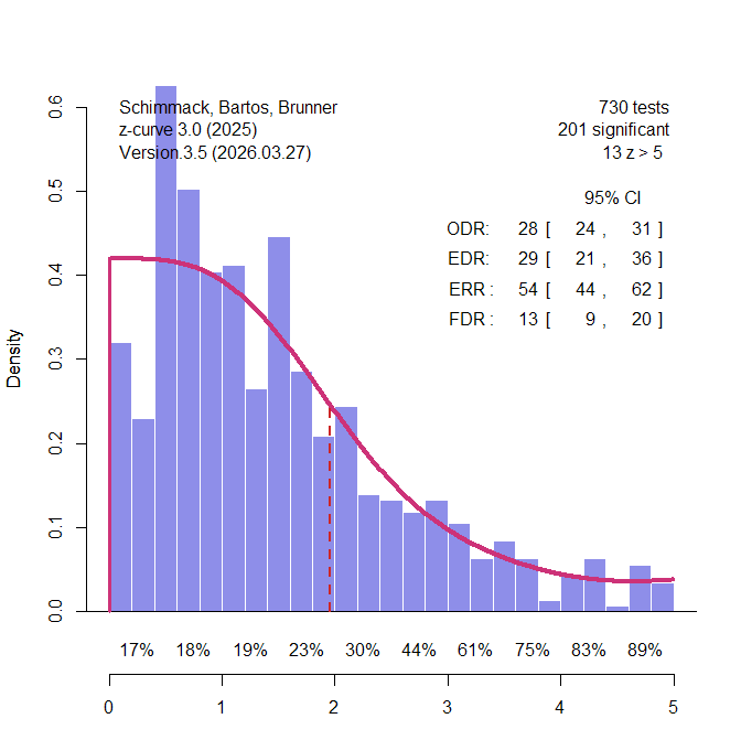
I converted power values into z-values and analyzed the z-values with z-curve.3.0 using the default model (Figure 1).

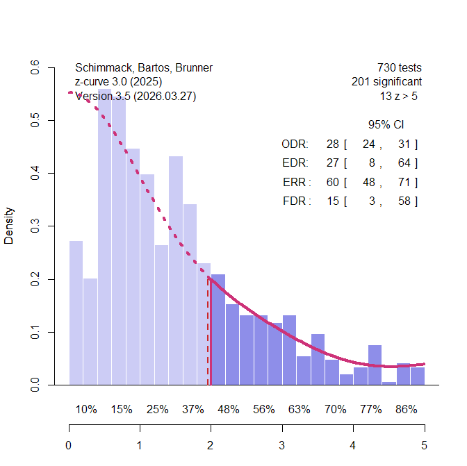
The observed discovery rate (ODR) is simply the percentage of significant results. More important is the bias-corrected estimate of unconditional mean power for all 730 z-values. Z-curve uses the observed distribution of significant z-values and projects the fitted model into the range of unobserved significant results. As shown in Figure 1, the model predicts the actual distribution of non-significant results fairly well. This suggests that the use of meta-analytic effect sizes adjusted inflated effect size estimates and removed publication bias. The estimated mean power for all studies is called the expected discovery rate (EDR). The EDR estimate is close to the ODR, suggesting further that the data are unbiased.

A key problem of estimating the EDR based on the significant results only is that the confidence interval around the point estimate is very wide. When the data show no major bias, more precise estimates can be obtained by fitting the model to all 730 data (Figure 2).

The key finding is that the point estimate of the false positive risk, FDR = 13% is in line with calculations based on Button’s estimate of mean power. The confidence interval around this estimate limits the FDR at 20%. This is an upper limit because conditional power of studies with significant results is likely to be less than 100%.

In fact, z-curve makes it possible to estimate conditional power of significant studies. First, z-curve estimates unconditional average power of significant studies. This parameter is called the expected replication rate (ERR) because it predicts how many studies would produce a significant result again in a hypothetical replication project that reproduces the original studies exactly with new samples. The ERR is 54% with an upper limit of 60% for the 95% confidence interval. We also know that no more than 20% of these studies are false positives. Assuming 80% true hypotheses, the average conditional power can not be higher than (.60 – .20*.05) / .8 = 74%. Thus, Soric’s assumption of 100% power is conservative, and the false positive rate is likely to be lower.

In conclusion, a z-curve analysis of Nord et al.’s power estimates for Button et al.’s meta-analyses confirms estimates that could have been obtained by applying Soric’s formula to Button et al.’s estimate of mean power. The true rate of false positive results remains unknown, but it is unlikely to be more than 20%.

Heterogeneity Across Research Areas

Nord et al. (2017) demonstrated that power varies across different research areas that were included in Button et al.’s sample of meta-analyses. Some of these areas had enough studies to conduct z-curve analyses for these specific areas. The most interesting area are candidate-gene studies that relate genotypic variation in single genes to phenotypes across participants With the benefit of hindsight, it is known that variation in a single gene has trivial effects on complex traits and that many of the significant results in these studies were practically false positive results (Duncan & Keller, 2011). 234 of the 730 studies were from this research area. Figure 3 shows the results. Interestingly, only 11% of the results were statistically significant. Thus, the low average power can be explained by many studies that reported non-significant results. There is no evidence of publication bias in these meta-analyses.

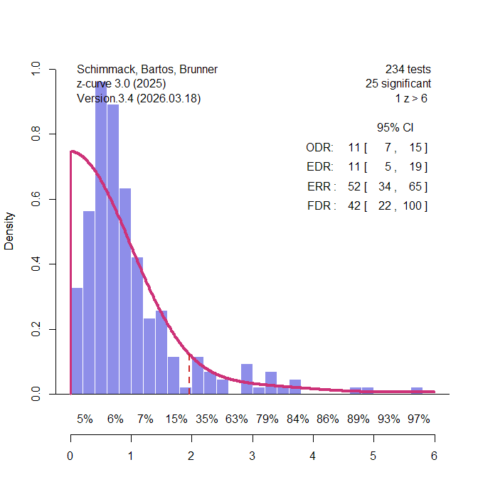
Using Soric’s formula, the low EDR translates into a high false positive risk, 42% and the upper limit of the 95% confidence interval includes 100%. Thus, z-curve confirms that the rare significant results in this literature could be false positive results. Most significant results also are just significant. There are hardly any results that show strong evidence (z > 4) against the null-hypothesis.

In short, a large portion of the 730 studies came from a research area that is known to have produced few significant results. This finding implies that other research areas are producing more credible significant results (Nord et al., 2017).

A second set of meta-analyses were clinical trials. Clinical trials have received considerable attention using Cochrane meta-analyses and abstracts in original articles that often report the key statistical result ( (Jager & Leek, 2013; Schimmack & Bartos, 2023, van Zwet et al., 2024). The results suggest that unconditional mean power is around 30% and the false positive risk is between 10% and 20%. These results serve as benchmarks for the z-curve analysis of the 145 clinical trials in Button et al.’s study (Figure 4).

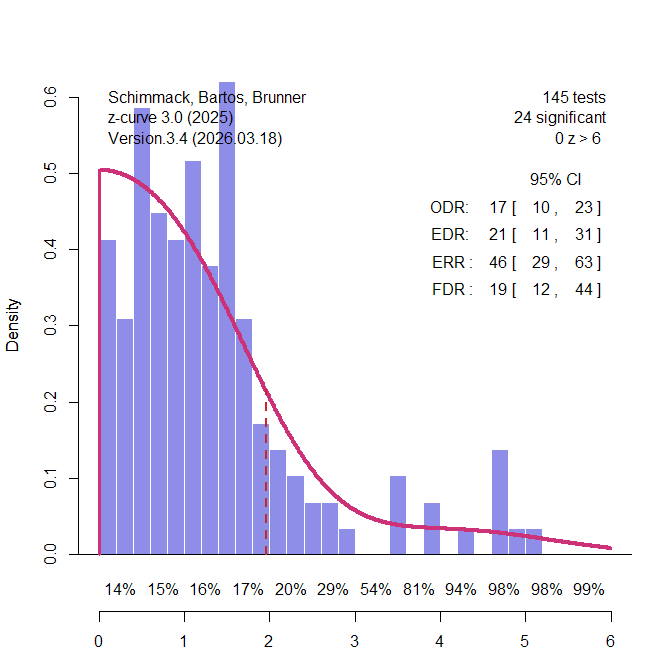
The EDR is somewhat lower, 21%, but the 95% confidence interval includes 30%. The FDR is 19%, but the lower limit of the confidence interval includes 13%. Thus, the results are a bit lower, but mostly consistent with evidence from estimates based on thousands of results. These estimates of the FDR are notably lower than the false positive rates that were predicted by Ioannidis’s scenarios that assumed high rates of true null-hypotheses.

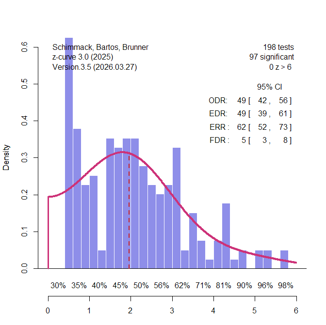
The third domain were studies from psychology. Psychological scientists have examined the credibility of their research in the wake of replication failures (Open Science Collaboration, 2015). Suddenly, only significant results in multiple studies within a single study were no longer attributed to reliable effects, but seen as signs of selection for significance (Schimmack, 2012). Francis (2014) found that over 80% of these multi-study articles showed statistically significant evidence of bias. Large scale multi-lab replication studies failed also showed that effect sizes estimates in these studies could be inflated by a factor of 1,000, shrinking effect sizes from d = .6 to d = .06 (Vohs et al., 2019). A z-curve analysis of a representative sample of studies in social psychology estimated that average unconditional power before selection for significance, EDR = 19%, FDR = 22%. Cohen (1962) already found similar estimates are similar for focal and non-focal results. This was also the case in a survey of emotion research (Soto & Schimmack, 2024). Soto and Schimmack (2024) reported an EDR of 30% and a corresponding FDR = 12% (k sig = 21,628) for all automatically extracted tests, and an EDR of 27%, FDR = 14%, for hand-coded focal tests (k sig = 227). These results serve as a comparison standard for the z-curve of 145 studies classified as psychological research by Nord et al. (2017). The EDR is 49%, FDR = 5%. Even the lower limit of the EDR confidence interval, 39%, implies only 8% false positives. among the significant results.

There are several reasons why these results differ from other findings. First, the focus on meta-analyses leads to an unrepresentative sample of the entire literature. Meta-analyses often include a lot more non-significant results and have less bias than original articles. Second, the specific set of meta-analyses was not representative of the broader literature in psychology. Thus, the results cannot be generalized from the specific studies in Button et al.’s sample to psychology or neuroscience. That would require representative sampling or collecting data from all studies using automatic extraction of test statistics.

Discussion

Button et al.’s (2013) was a first attempt to assess the credibility of empirical results with empirical estimates of power based on meta-analytic effect sizes and sample sizes. The median power was low (21%). The key implications of these finding was that researchers often fail to reject null-hypotheses and may use questionable research practices to report significant results in published articles. Low power and bias could lead to many false positive results. This article added to other concerns about the reliability of findings in neuroscience (Vul et al., 2019).

Most citations took Button et al.’s findings and implications at face value. Nord et al. (2017) pointed out that power and false positive rates varied across research areas. Most notably, candidate gene studies have lower power and a much higher false positive risk. Including these studies in the calculation of median power may have led to false perceptions of other research areas.

Here I presented the first serious critical examination of Button et al.’s methodology and inferences and found several problems that undermine their pessimistic assessment of neuroscience. First, they estimated unconditional power, but their false positive calculations require estimates of conditional power. Second, false positives rates depend on mean power and not median power. Mean power was 35% which is close to the estimate for psychology based on actual replication studies (OSC, 2015). Third, they made unnecessary assumptions about ratios of true and false hypotheses being tested, when unconditional power alone is sufficient to estimate false positive rates (Soric, 1989). Fourth, they relied on meta-analysis to correct for publication bias, but meta-analyses are not representative of the broader literature.

Meta-science is like other sciences. Ideally, critical analyses reveal problems and new innovations address these problems. Power estimation started in the 1960s with Cohen’s seminal article. Cohen (1962) worked with plausible effect sizes, but did not aim to estimate studies true power. Moreover, his work and statistical power were largely ignored (Cohen, 1990; Sedlmeier & Gigenzer, 1989).

Conclusion

The replication crisis stimulated renewed interest in methods that use observed results to draw inferences about the power of actual studies (Ioannidis & Trikalinos, 2007; Francis, 2014; Schimmack, 2012; Simonsohn, Nelson, & Simmons, 2014). This work shifted attention from prospective power calculations to the retrospective assessment of evidential strength in published literatures. Two challenges emerged as central. First, selection bias inflates the observed rate of significant results, requiring methods that correct for selection. Second, power varies across studies, requiring models that allow for heterogeneity rather than assuming a single common effect size or power level. Early approaches addressed selection under simplifying assumptions, typically treating power as homogeneous across studies. As a result, their inferences become unreliable when studies differ in sample size, effect size, or both (Brunner & Schimmack, 2020; Schimmack, 2026).

Z-curve extends this line of work by explicitly modeling both selection and heterogeneity, estimating a distribution of power across studies rather than a single average. This provides a framework for quantifying key properties of the literature, including expected discovery and replication rates, and for linking these quantities to false discovery risk (Sorić, 1989). In this sense, z-curve represents a substantive advance in the empirical assessment of the credibility of published findings. Like earlier contributions such as Button et al., it is unlikely to be the final word, but it is currently the most advanced method to estimate true power for sets of studies with heterogeneity in power and selection bias.

Meta-Analysis of Observed Power: Comparison of Estimation Methods

April 1, 2015Median Observed Power, Meta-Analysis, Observed Power, Pcurve, Post-Hoc Power, Posteriori Power Analysis, Publication Bias, Puniform, Questionable Research Practices, r-index, YMCA, Yuan-Maxwell, Yuan-Maxwell Correction, Yuan-Maxwell-Corrected-AverageMeta-Analysis, Meta-Science, replicability, Replication, ScienceUlrich Schimmack

Meta-Analysis of Observed Power

Citation: Dr. R (2015). Meta-analysis of observed power. R-Index Bulletin, Vol(1), A2.

In a previous blog post, I presented an introduction to the concept of observed power. Observed power is an estimate of the true power on the basis of observed effect size, sampling error, and significance criterion of a study. Yuan and Maxwell (2005) concluded that observed power is a useless construct when it is applied to a single study, mainly because sampling error in a single study is too large to obtain useful estimates of true power. However, sampling error decreases as the number of studies increases and observed power in a set of studies can provide useful information about the true power in a set of studies.

This blog post introduces various methods that can be used to estimate power on the basis of a set of studies (meta-analysis). I then present simulation studies that compare the various estimation methods in terms of their ability to estimate true power under a variety of conditions. In this blog post, I examine only unbiased sets of studies. That is, the sample of studies in a meta-analysis is a representative sample from the population of studies with specific characteristics. The first simulation assumes that samples are drawn from a population of studies with fixed effect size and fixed sampling error. As a result, all studies have the same true power (homogeneous). The second simulation assumes that all studies have a fixed effect size, but that sampling error varies across studies. As power is a function of effect size and sampling error, this simulation models heterogeneity in true power. The next simulations assume heterogeneity in population effect sizes. One simulation uses a normal distribution of effect sizes. Importantly, a normal distribution has no influence on the mean because effect sizes are symmetrically distributed around the mean effect size. The next simulations use skewed normal distributions. This simulation provides a realistic scenario for meta-analysis of heterogeneous sets of studies such as a meta-analysis of articles in a specific journal or articles on different topics published by the same author.

Observed Power Estimation Method 1: The Percentage of Significant Results

The simplest method to determine observed power is to compute the percentage of significant results. As power is defined as the long-range percentage of significant results, the percentage of significant results in a set of studies is an unbiased estimate of the long-term percentage. The main limitation of this method is that the dichotomous measure (significant versus insignificant) is likely to be imprecise when the number of studies is small. For example, two studies can only show observed power values of 0, 25%, 50%, or 100%, even if true power were 75%. However, the percentage of significant results plays an important role in bias tests that examine whether a set of studies is representative. When researchers hide non-significant results or use questionable research methods to produce significant results, the percentage of significant results will be higher than the percentage of significant results that could have been obtained on the basis of the actual power to produce significant results.

Observed Power Estimation Method 2: The Median

Schimmack (2012) proposed to average observed power of individual studies to estimate observed power. Yuan and Maxwell (2005) demonstrated that the average of observed power is a biased estimator of true power. It overestimates power when power is less than 50% and it underestimates true power when power is above 50%. Although the bias is not large (no more than 10 percentage points), Yuan and Maxwell (2005) proposed a method that produces an unbiased estimate of power in a meta-analysis of studies with the same true power (exact replication studies). Unlike the average that is sensitive to skewed distributions, the median provides an unbiased estimate of true power because sampling error is equally likely (50:50 probability) to inflate or deflate the observed power estimate. To avoid the bias of averaging observed power, Schimmack (2014) used median observed power to estimate the replicability of a set of studies.

Observed Power Estimation Method 3: P-Curve’s KS Test

Another method is implemented in Simonsohn’s (2014) pcurve. Pcurve was developed to obtain an unbiased estimate of a population effect size from a biased sample of studies. To achieve this goal, it is necessary to determine the power of studies because bias is a function of power. The pcurve estimation uses an iterative approach that tries out different values of true power. For each potential value of true power, it computes the location (quantile) of observed test statistics relative to a potential non-centrality parameter. The best fitting non-centrality parameter is located in the middle of the observed test statistics. Once a non-central distribution has been found, it is possible to assign each observed test-value a cumulative percentile of the non-central distribution. For the actual non-centrality parameter, these percentiles have a uniform distribution. To find the best fitting non-centrality parameter from a set of possible parameters, pcurve tests whether the distribution of observed percentiles follows a uniform distribution using the Kolmogorov-Smirnov test. The non-centrality parameter with the smallest test statistics is then used to estimate true power.

Observed Power Estimation Method 4: P-Uniform

van Assen, van Aert, and Wicherts (2014) developed another method to estimate observed power. Their method is based on the use of the gamma distribution. Like the pcurve method, this method relies on the fact that observed test-statistics should follow a uniform distribution when a potential non-centrality parameter matches the true non-centrality parameter. P-uniform transforms the probabilities given a potential non-centrality parameter with a negative log-function (-log[x]). These values are summed. When probabilities form a uniform distribution, the sum of the log-transformed probabilities matches the number of studies. Thus, the value with the smallest absolute discrepancy between the sum of negative log-transformed percentages and the number of studies provides the estimate of observed power.

Observed Power Estimation Method 5: Averaging Standard Normal Non-Centrality Parameter

In addition to these existing methods, I introduce to novel estimation methods. The first new method converts observed test statistics into one-sided p-values. These p-values are then transformed into z-scores. This approach has a long tradition in meta-analysis that was developed by Stouffer et al. (1949). It was popularized by Rosenthal during the early days of meta-analysis (Rosenthal, 1979). Transformation of probabilities into z-scores makes it easy to aggregate probabilities because z-scores follow a symmetrical distribution. The average of these z-scores can be used as an estimate of the actual non-centrality parameter. The average z-score can then be used to estimate true power. This approach avoids the problem of averaging power estimates that power has a skewed distribution. Thus, it should provide an unbiased estimate of true power when power is homogenous across studies.

Observed Power Estimation Method 6: Yuan-Maxwell Correction of Average Observed Power

Yuan and Maxwell (2005) demonstrated a simple average of observed power is systematically biased. However, a simple average avoids the problems of transforming the data and can produce tighter estimates than the median method. Therefore I explored whether it is possible to apply a correction to the simple average. The correction is based on Yuan and Maxwell’s (2005) mathematically derived formula for systematic bias. After averaging observed power, Yuan and Maxwell’s formula for bias is used to correct the estimate for systematic bias. The only problem with this approach is that bias is a function of true power. However, as observed power becomes an increasingly good estimator of true power in the long run, the bias correction will also become increasingly better at correcting the right amount of bias.

The Yuan-Maxwell correction approach is particularly promising for meta-analysis of heterogeneous sets of studies such as sets of diverse studies in a journal. The main advantage of this method is that averaging of power makes no assumptions about the distribution of power across different studies (Schimmack, 2012). The main limitation of averaging power was the systematic bias, but Yuan and Maxwell’s formula makes it possible to reduce this systematic bias, while maintaining the advantage of having a method that can be applied to heterogeneous sets of studies.

RESULTS

Homogeneous Effect Sizes and Sample Sizes

The first simulation used 100 effect sizes ranging from .01 to 1.00 and 50 sample sizes ranging from 11 to 60 participants per condition (Ns = 22 to 120), yielding 5000 different populations of studies. The true power of these studies was determined on the basis of the effect size, sample size, and the criterion p < .025 (one-tailed), which is equivalent to .05 (two-tailed). Sample sizes were chosen so that average power across the 5,000 studies was 50%. The simulation drew 10 random samples from each of the 5,000 populations of studies. Each sample of a study simulated a between-subject design with the given population effect size and sample size. The results were stored as one-tailed p-values. For the meta-analysis p-values were converted into z-scores. To avoid biases due to extreme outliers, z-scores greater than 5 were set to 5 (observed power = .999).

The six estimation methods were then used to compute observed power on the basis of samples of 10 studies. The following figures show observed power as a function of true power. The green lines show the 95% confidence interval for different levels of true power. The figure also includes red dashed lines for a value of 50% power. Studies with more than 50% observed power would be significant. Studies with less than 50% observed power would be non-significant. The figures also include a blue line for 80% true power. Cohen (1988) recommended that researchers should aim for a minimum of 80% power. It is instructive how accurate estimation methods are in evaluating whether a set of studies met this criterion.

The histogram shows the distribution of true power across the 5,000 populations of studies.

The histogram shows that the simulation covers the full range of power. It also shows that high-powered studies are overrepresented because moderate to large effect sizes can achieve high power for a wide range of sample sizes. The distribution is not important for the evaluation of different estimation methods and benefits all estimation methods equally because observed power is a good estimator of true power when true power is close to the maximum (Yuan & Maxwell, 2005).

The next figure shows scatterplots of observed power as a function of true power. Values above the diagonal indicate that observed power overestimates true power. Values below the diagonal show that observed power underestimates true power.

Visual inspection of the plots suggests that all methods provide unbiased estimates of true power. Another observation is that the count of significant results provides the least accurate estimates of true power. The reason is simply that aggregation of dichotomous variables requires a large number of observations to approximate true power. The third observation is that visual inspection provides little information about the relative accuracy of the other methods. Finally, the plots show how accurate observed power estimates are in meta-analysis of 10 studies. When true power is 50%, estimates very rarely exceed 80%. Similarly, when true power is above 80%, observed power is never below 50%. Thus, observed power can be used to examine whether a set of studies met Cohen’s recommended guidelines to conduct studies with a minimum of 80% power. If observed power is 50%, it is nearly certain that the studies did not have the recommended 80% power.

To examine the relative accuracy of different estimation methods quantitatively, I computed bias scores (observed power – true power). As bias can overestimate and underestimate true power, the standard deviation of these bias scores can be used to quantify the precision of various estimation methods. In addition, I present the mean to examine whether a method has large sample accuracy (i.e. the bias approaches zero as the number of simulations increases). I also present the percentage of studies with no more than 20% points bias. Although 20% bias may seem large, it is not important to estimate power with very high precision. When observed power is below 50%, it suggests that a set of studies was underpowered even if the observed power estimate is an underestimation.

The quantitative analysis also shows no meaningful differences among the estimation methods. The more interesting question is how these methods perform under more challenging conditions when the set of studies are no longer exact replication studies with fixed power.

Homogeneous Effect Size, Heterogeneous Sample Sizes

The next simulation simulated variation in sample sizes. For each population of studies, sample sizes were varied by multiplying a particular sample size by factors of 1 to 5.5 (1.0, 1.5,2.0…,5.5). Thus, a base-sample-size of 40 created a range of sample sizes from 40 to 220. A base-sample size of 100 created a range of sample sizes from 100 to 2,200. As variation in sample sizes increases the average sample size, the range of effect sizes was limited to a range from .004 to .4 and effect sizes were increased in steps of d = .004. The histogram shows the distribution of power in the 5,000 population of studies.

The simulation covers the full range of true power, although studies with low and very high power are overrepresented.

The results are visually not distinguishable from those in the previous simulation.

The quantitative comparison of the estimation methods also shows very similar results.

In sum, all methods perform well even when true power varies as a function of variation in sample sizes. This conclusion may not generalize to more extreme simulations of variation in sample sizes, but more extreme variations in sample sizes would further increase the average power of a set of studies because the average sample size would increase as well. Thus, variation in effect sizes poses a more realistic challenge for the different estimation methods.

Heterogeneous, Normally Distributed Effect Sizes

The next simulation used a random normal distribution of true effect sizes. Effect sizes were simulated to have a reasonable but large variation. Starting effect sizes ranged from .208 to 1.000 and increased in increments of .008. Sample sizes ranged from 10 to 60 and increased in increments of 2 to create 5,000 populations of studies. For each population of studies, effect sizes were sampled randomly from a normal distribution with a standard deviation of SD = .2. Extreme effect sizes below d = -.05 were set to -.05 and extreme effect sizes above d = 1.20 were set to 1.20. The first histogram of effect sizes shows the 50,000 population effect sizes. The histogram on the right shows the distribution of true power for the 5,000 sets of 10 studies.

The plots of observed and true power show that the estimation methods continue to perform rather well even when population effect sizes are heterogeneous and normally distributed.

The quantitative comparison suggests that puniform has some problems with heterogeneity. More detailed studies are needed to examine whether this is a persistent problem for puniform, but given the good performance of the other methods it seems easier to use these methods.

Heterogeneous, Skewed Normal Effect Sizes

The next simulation puts the estimation methods to a stronger challenge by introducing skewed distributions of population effect sizes. For example, a set of studies may contain mostly small to moderate effect sizes, but a few studies examined large effect sizes. To simulated skewed effect size distributions, I used the rsnorm function of the fGarch package. The function creates a random distribution with a specified mean, standard deviation, and skew. I set the mean to d = .2, the standard deviation to SD = .2, and skew to 2. The histograms show the distribution of effect sizes and the distribution of true power for the 5,000 sets of studies (k = 10).

This time the results show differences between estimation methods in the ability of various estimation methods to deal with skewed heterogeneity. The percentage of significant results is unbiased, but is imprecise due to the problem of averaging dichotomous variables. The other methods show systematic deviations from the 95% confidence interval around the true parameter. Visual inspection suggests that the Yuan-Maxwell correction method has the best fit.

This impression is confirmed in quantitative analyses of bias. The quantitative comparison confirms major problems with the puniform estimation method. It also shows that the median, p-curve, and the average z-score method have the same slight positive bias. Only the Yuan-Maxwell corrected average power shows little systematic bias.

To examine biases in more detail, the following graphs plot bias as a function of true power. These plots can reveal that a method may have little average bias, but has different types of bias for different levels of power. The results show little evidence of systematic bias for the Yuan-Maxwell corrected average of power.

The following analyses examined bias separately for simulation with less or more than 50% true power. The results confirm that all methods except the Yuan-Maxwell correction underestimate power when true power is below 50%. In contrast, most estimation methods overestimate true power when true power is above 50%. The exception is puniform which still underestimated true power. More research needs to be done to understand the strange performance of puniform in this simulation. However, even if p-uniform could perform better, it is likely to be biased with skewed distributions of effect sizes because it assumes a fixed population effect size.

Conclusion

This investigation introduced and compared different methods to estimate true power for a set of studies. All estimation methods performed well when a set of studies had the same true power (exact replication studies), when effect sizes were homogenous and sample sizes varied, and when effect sizes were normally distributed and sample sizes were fixed. However, most estimation methods were systematically biased when the distribution of effect sizes was skewed. In this situation, most methods run into problems because the percentage of significant results is a function of the power of individual studies rather than the average power.

The results of these analyses suggest that the R-Index (Schimmack, 2014) can be improved by simply averaging power and then applying the Yuan-Maxwell correction. However, it is important to realize that the median method tends to overestimate power when power is greater than 50%. This makes it even more difficult for the R-Index to produce an estimate of low power when power is actually high. The next step in the investigation of observed power is to examine how different methods perform in unrepresentative (biased) sets of studies. In this case, the percentage of significant results is highly misleading. For example, Sterling et al. (1995) found percentages of 95% power, which would suggest that studies had 95% power. However, publication bias and questionable research practices create a bias in the sample of studies that are being published in journals. The question is whether other observed power estimates can reveal bias and can produce accurate estimates of the true power in a set of studies.

Replicability-Index

Improving the replicability of empirical research