Since Cohen (1962) published his famous article on statistical power in psychological journals, statistical power has not increased. The R-Index makes it possible f to distinguish studies with high power (good science) and studies with low power (bad science). Protect yourself from bad science and check the R-Index before you believe statistical results.
View all posts by Ulrich Schimmack →
Peer review is supposed to uncover errors in manuscripts. Sometimes it does. Sometimes it provides a rather nice demonstration of the errors humans make while trying to find errors in other people’s work.
I recently submitted a manuscript on publication-bias detection in meta-analysis. The central empirical result was simple: tests of publication bias often have low power when effects are heterogeneous and model assumptions are violated. Consequently, a nonsignificant test for publication bias should not be interpreted as evidence that publication bias is absent. The paper therefore argued for estimating how much publication bias remains compatible with the data, rather than relying on binary significance tests.
The paper was rejected. In his editorial letter, Associate Editor Stephen West wrote that there were “several statistical misstatements throughout the paper which need to be corrected.”
That sounds serious. So I went back through the reviews to identify these errors.
The exercise turned out to be more interesting than expected.
Error 1: What is statistical power?
The manuscript stated:
“Classical power is conditional on the null hypothesis being false and on a specified population effect size being the true effect size.”
Reviewer 2 responded:
“This is false. See a basic introductory statistics textbook such as Testing Statistical Hypotheses by Lehmann and Romano.”
This criticism is particularly interesting because it directly contradicts another criticism of my work that I tried to estimate “average power” without conditioning on a true effect size.
In other words, I was first criticized because power is conditional, I changed the terminology accordingly, and now I am now criticized because defining power as conditional is supposedly false.
Welcome to psycho-science.
Part of the confusion is historical. Lehmann’s Testing Statistical Hypotheses, first published in 1959, uses the classical mathematical-statistics concept of a power function, which gives the probability of rejecting the null as a function of the population parameter and can therefore be evaluated both under the null and under alternatives. That terminology was retained in later editions. In contemporary psychological research, however, statistical power is ordinarily used more narrowly for the probability of rejecting the null conditional on a specified alternative effect size—a usage central to prospective sample-size planning (e.g., Pek et al., 2024).
Maria Soto and I recently published a power primer specifically to disentangle these different usages of power (Soto & Schimmack, 2026). So the problem here is not that I fail to understand conditional probabilities. The problem is that different statistical traditions use the same word differently. It is particularly unhelpful for a reviewer to take one legitimate historical usage and declare another established usage simply “false” and for a lazy editor to repeat this claim without being aware that the term power has no clear definition in the psychological literature.
Error 2: You cannot manipulate the number of significant studies or the FDR
Reviewer 1 objected to two factors in the simulation:
“I don’t see that you can directly vary the number of significant studies or the FDR.”
Of course you can.
A simulation does not have to start with a fixed number of attempted studies and then passively accept whatever number of significant findings happens to emerge. One can condition the simulation on the evidence of interest.
If I want 300 significant results with an FDR of .20, I can generate 60 significant results under the null and 240 significant results under alternatives. This is no more mysterious than fixing the sample size, heterogeneity, or mixture proportions in any other simulation.
Whether this is a useful simulation design is a legitimate question.
Whether it is possible is not.
The reviewer additionally wrote that they did not see the relevance of FDR to meta-analysis. That is a substantive theoretical position. It effectively assumes that a heterogeneous literature should be represented as a continuous distribution of nonzero effects rather than as a mixture that can include true null effects.
But one purpose of the simulation was precisely to avoid making that assumption. The replication crisis has made it entirely plausible that some proportion of published significant findings are false positives. If that possibility is excluded by design, then publication-bias methods are being evaluated only in a world in which every study investigates a real nonzero effect. That is a very strong assumption to build into a simulation of publication bias.
Error 3: Zero effects make high power impossible
The manuscript reported:
“No method approached the conventional .80 benchmark when averaged across the full design.”
Reviewer 1 responded:
“But the full design includes zero effect sizes, doesn’t it? … So no test would have .80 power under those conditions.”
Here the reviewer has confused two entirely different meanings of power.
The quantity being evaluated was the power of a publication-bias test: if a simulated data set is biased, what is the probability that the test correctly rejects the null hypothesis of no publication bias?
It was not the power of the original studies to reject a substantive null hypothesis.
A literature in which every population effect is zero can nevertheless provide overwhelming evidence of publication bias. Suppose only 5% of results would normally be significant, but nearly all nonsignificant findings disappear. With enough observations, a publication-bias test could have very high power to detect that selection.
Thus, including studies with true null effects does not make .80 power impossible. If anything, strong selection is easier to detect when the underlying discovery rate is low, because publication bias produces a large distortion in the observed proportion and distribution of significant results. By contrast, when studies already have high power and most results are significant before selection, removing nonsignificant studies produces a much smaller observable distortion and publication bias becomes harder to detect.
Error 4: 5,184 simulation conditions is a miscalculation
Reviewer 2 wrote:
“The paper reports 5,184 conditions. I count 3 number of studies × 4 effect sizes × 3 heterogeneity values × 3 sample sizes × 4 FDRs × 3 publication bias settings which gets me to 1,728 so off by a factor of three. What am I missing?”
What was missing was one of the simulation factors: the three distributions of population effects.
The design was 3 x 4 x 4 x 3 x 4 x 3 x 3 = 5,184.
There were four, not three, levels of heterogeneity, and three effect-distribution conditions.
There is another small problem. Even the multiplication printed in the review, 3 x 4 x 3 x 3 x 4 x 3 equals 1,296, not 1,728.
So this particular attempt to identify an arithmetic error contains an arithmetic error.
Error 5: A beta distribution cannot have mean zero
Error 5: A beta distribution cannot have mean zero
Here the reviewers found a real problem.
The manuscript described a Beta(1,10) distribution as having mean 0 and standard deviation .4. A raw Beta(1,10) distribution obviously does not have those moments.
The problem, however, was in the description of the simulation, not in the simulation itself. The beta distribution was used to generate the shape of the effect-size distribution and was then transformed to have the intended mean and standard deviation. The manuscript failed to describe that transformation clearly.
In the era of open science, this distinction is unusually easy to resolve. The simulation code was available, so a reviewer who suspected that the reported moments were impossible could have checked whether the error was in the prose or in the actual data-generating process. The code shows that the simulation itself implemented the intended transformed distribution.
So this was a genuine reporting error that peer review correctly detected. But it was not evidence that the simulation results were based on an incorrectly specified Beta(1,10) distribution.
Error 6: The mysterious noncentrality parameter
Another reviewer objected to the statement that a simulated z statistic had a noncentrality parameter of 2:
“There is no noncentrality parameter for a normal distribution. Presumably the mean was 2?”
This is mostly terminology. Under an alternative hypothesis, a normal distribution is centered over a value other than zero. If all studies have 50% power with a significance criterion value of 1.96, the distribution is centered at 1.96 (~ 2).
In power calculations this quantity is routinely described as the noncentrality parameter, although unlike the t, F, and chi-square families there is no separately named “noncentral normal distribution.”
Calling it the mean of the alternative z distribution would avoid the terminological distraction. Call it what you want, but all sampling distributions have a median and when the effect size is not zero, the median is not zero. Whatever you call it, everybody can understand the meaning here and maybe propose a wording change rather than claiming that I invented a statistical entity that does not exist.
Again, this is very different from discovering that the simulation or its conclusions are wrong.
What was actually wrong?
After going through the reviews, I can identify one clear reporting problem: the description of the transformed beta distribution. There are also several places where the manuscript could have been clearer—the z-curve version numbers were particularly unhelpful, and some terminology could be tightened.
Those are useful comments.
Other alleged errors fare less well. The number of simulation conditions was correct. It is perfectly possible to condition a simulation on the number and composition of significant studies. Including zero population effects does not make it impossible for a publication-bias test to have high power. And the definition of power that one reviewer declared “false” is closely related to the very definition that other critics previously insisted I adopt.
None of this proves that the manuscript deserved acceptance. The paper was too long. Its argument could have been more focused. Including a conventional multi-step selection model would strengthen the comparison. The presentation of the various z-curve versions invited confusion.
These are legitimate criticisms.But those are different claims from saying that the paper contained “several statistical misstatements.”
ut those are different claims from saying that the paper contained “several statistical misstatements.”
There is also a simple reason why the manuscript contains no major statistical errors. Before submitting it, I used AI—both ChatGPT and Claude—to challenge my arguments, check calculations, and look for weaknesses. AI did not write the ideas for me, but it was extremely useful as an adversarial reader.
After receiving the reviews, I conducted a small experiment. I uploaded the anonymous manuscript to Claude and presented the reviews as if they were drafts of reviews that I had written and wanted evaluated. Claude was not particularly impressed. (It eventually figured out what was going on because it located the preprint with my name on it.)
Reviewer 1
“Your review raises several valid concerns, but about a third of the specific comments contain an error or overreach that the author could easily rebut. It also misses some issues that are stronger than the ones it leads with. My suggestions are below, in order of importance.”
Reviewer 2
“Reviewer 2 raises the most damaging points in either review: whether z-curve has been properly vetted, and the coverage claim. Several of the supporting comments, though, are factually off or point at the wrong target, and the author could rebut them easily.”
Conclusion
Peer review is commonly described as quality control, but anonymous peer review does not guarantee quality control. It is a human judgment process, and human judges make mistakes. Reviewers misunderstand arguments, overlook information, perform arithmetic incorrectly, import their own theoretical commitments, and sometimes mistake disagreements about terminology or modeling assumptions for factual errors.
Editors then have to evaluate those reviews. If they do not independently check the reviewers’ claims, reviewer errors can become editorial “facts.” In this case, an editorial decision referred to “several statistical misstatements,” even though several of the alleged mistakes were themselves mistakes in the reviews.
This is where AI changes the scientific publishing system. An AI system can read a manuscript, inspect a review, check arithmetic, distinguish a factual error from a modeling disagreement, and compare a criticism with the actual contents of the manuscript in seconds. It will also make mistakes, of course. But unlike traditional peer review, those judgments can be generated repeatedly, compared across systems, and audited immediately.
The interesting question is therefore no longer whether AI should be allowed into peer review. It is already better than pretending that two anonymous humans constitute a reliable error-detection system.
Journals may increasingly use AI to assist editors and reviewers. Authors will certainly use it to evaluate reviews. And eventually the importance of journal gatekeeping itself may decline. Scientific papers increasingly function as inputs into larger information systems—search engines, databases, systematic reviews, and now AI models—that integrate evidence across sources rather than treating publication in a particular journal as the final certificate of truth.
Peer review will probably survive. But its monopoly on deciding what counts as credible scientific information may not.
AI may eventually kill us, but I hope it will kill bad peer reviews first.
Alesina, A., Carlana, M., La Ferrara, E., & Pinotti, P. (2018). Revealing stereotypes: Evidence from immigrants in schools (NBER Working Paper No. 25333). National Bureau of Economic Research. https://doi.org/10.3386/w25333
Abstracts are short and cannot tell the whole story. A previous working paper and data in this article show that the IAT was also used to predict grading and that there was no evidence that IAT scores predicted lower grades for immigrant students.
The study
Alesina, Carlana, La Ferrara and Pinotti asked whether Italian middle-school teachers’ implicit stereotypes about immigrants, measured with an immigrant/Italian-name IAT, show up in how they grade immigrant students. They also asked whether telling teachers their IAT scores changes their grading.
The design has real strengths:
1,384 teachers in 102 schools took the IAT.
Grades came from administrative records, so teachers didn’t know their grading was being observed.
Blind-graded national tests (INVALSI) provide a performance benchmark.
A randomized field experiment varied when teachers received their IAT feedback.
The paper circulated as NBER Working Paper 25333 (December 2018). It was published in the American Economic Review in July 2024. Between the two versions, the evidence on the central predictive-validity question changed little, but the presentation changed a lot.
The predictive-validity test
The key analysis regresses end-of-year grades on an Immigrant × Teacher-IAT interaction, controlling for INVALSI scores and teacher fixed effects. Grades are from the 2011–2016 cohorts. If the IAT measures something that drives discriminatory grading, teachers with higher scores should show a larger immigrant penalty at equal test performance.
Working paper (2018). The authors analyzed math and literature separately.
For math, one SD higher on the IAT (0.26 D-units) was associated with a 0.033-point larger immigrant penalty (SE 0.019). This was significant only at p < .10 in every specification.
For literature, the estimate was zero (−0.001, SE 0.017).
The literature null was explained after the fact by lenience toward first-generation immigrants. The supporting interaction was itself not significant.
Published version (2024). The subjects are pooled, standard errors are clustered by teacher, and the IAT is entered in raw D-units.
The interaction is −0.075 (SE 0.050), p ≈ .13. The authors state that it is not statistically significant.
Per SD of IAT, that is about 0.02 grade points, or about 0.02 SD of grades.
The 95% CI excludes any effect larger than about 0.04 SD per SD of IAT.
So with a smallest effect of interest of d = .10, the data are evidence of no meaningful predictive validity, not merely a lack of evidence for it.
What changed between versions
1. The main test became a footnote to subgroup analyses. After the pooled null, the AER version splits students by INVALSI score.
For high-ability students: −0.139 (SE 0.080), p ≈ .08.
For low-ability students: −0.031 (SE 0.060).
No test of the difference between subgroups is reported.
Even the high-ability estimate implies at most about 0.07 SD per SD of IAT at the CI bound. This split does not appear in the working paper. Yet the abstract-level summary in the introduction now says that higher IAT scores are associated with lower grades for high-performing immigrants. The conclusion calls the pattern “strongly suggestive of bias.”
2. Measurement error was invoked, and a new measure was introduced. The authors attribute the null partly to noise in teacher-level bias estimates. In an online appendix, they show that a “naïve” teacher-level bias measure is not significantly related to the IAT. An empirical-Bayes-shrunken version of the same measure is. This alternative outcome appears only after the preregistered-looking specification fails, which is a classic forking path.
3. The measurement error that matters most is in the IAT itself. The AER version reports a new fact (footnote 6): the male-name and female-name immigrant IATs correlate only 0.28. That implies a reliability of roughly .44 for the averaged score. The authors present this as reassuring because 76% of teachers received consistent categorical feedback. But a test-retest correlation of .28 places a low ceiling on any criterion correlation. It also means many teachers were told they were “moderately” or “strongly” biased on the basis of noise.
4. The figures and text overstate the tables. The text describing Figure 5 says higher IAT is associated with significantly lower grades for immigrants. Table 3, which quantifies the same relationship, says it is not significant.
5. The framing moved from prediction to intervention. The working paper’s abstract led with the IAT–grading correlation. The AER abstract omits it and emphasizes the experiments. The working paper’s key moderator result—that the feedback effect was driven by teachers without explicit anti-immigrant views—has moved to an online appendix.
6. The IAT critique literature is acknowledged, then set aside. The AER version cites the predictive-validity critiques, including Blanton et al. (2009), Oswald et al. (2013), and Schimmack (2021). It responds that those studies used small samples and lacked real-world behavior. This study has a large sample and real-world behavior, and it reproduces the weak-to-null pattern those critiques describe.
The experiments
Field experiment. Receiving IAT feedback before grading narrowed the native–immigrant grade gap by 0.35 points (pooled ITT; SE 0.11). This is larger than the entire conditional gap the paper documents (about 0.10 points). It came from raising immigrants’ grades and lowering natives’ grades.
Did teachers with higher IAT scores respond more? The triple interaction is 0.214 (SE 0.302), which is null. In the field, the IAT predicts neither discrimination nor responsiveness to feedback. A reaction to being labeled biased explains the effect as well as correction of a bias does.
Online experiment. This was added for the AER version. Of 179 teachers who completed the survey, 146 are analyzed, and the attrition isn’t explained in the main text. Each teacher graded ten vignette tests with randomly assigned names.
The average effect of personalized feedback versus a generic debiasing message is zero (0.017, SE 0.122).
The headline result is a moderator effect: teachers with higher IAT scores responded more to their own feedback.
One result here does favor the IAT. In the active control group (about 74 teachers), higher IAT was associated with lower grades for immigrant-named tests (−0.426, SE 0.157). Three things should be weighed against it:
It comes from a small sample, in an exploratory interaction model.
The outcome is vignette grading, not real grades.
The group had just received a debiasing message, and teachers with IAT = 0 graded immigrant names 0.42 points higher than native names.
It does not replicate in the field data with real grades and about 780 teachers.
The AEA registry IDs (AEARCTR-0003647 and -0013570) appear to postdate the respective data collections. If so, the moderator analyses were not preregistered. This is worth confirming against the registry.
Conclusion
The working paper’s main predictive-validity claim was a marginal (p < .10) association in math and a null in literature. In the published version, with subjects pooled and errors clustered by teacher, the IAT does not significantly predict discriminatory grading. The estimate is small enough to rule out even modest effects.
The publication process did not converge on this conclusion. Instead it added subgroup splits, an alternative bias measure, and a second, small online experiment. That gave the final paper a narrative of implicit bias that is “strongly suggestive” in the conclusion but not supported by the primary test.
Two of the paper’s own facts deserve more attention than they received. First, about 70% of teachers have “moderate to severe” IAT scores, yet grading discrimination is about 0.1 points. Second, the two IATs given to the same teachers on the same day correlate .28. Both are hard to reconcile with the view that the IAT measures a stable implicit bias that shapes behavior.
In real classroom grading of immigrant students, the IAT failed to predict discrimination.
van Zwet, E., Gelman, A., Greenland, S., Imbens, G., Schwab, S., & Goodman, S. N. (2024). A New Look at P Values for Randomized Clinical Trials. NEJM evidence, 3(1), EVIDoa2300003. https://doi.org/10.1056/EVIDoa2300003
Introduction
Randomized controlled trials occupy a privileged position in evidence-based medicine because randomization protects against many sources of confounding that complicate observational research. Yet influential critics have questioned whether even randomized evidence can be trusted at face value. Ioannidis’s Why Most Published Research Findings Are False argued that low power, bias, and low prior probabilities can make statistically significant findings more likely to be false than true, and his argument explicitly included clinical trials (Ioannidis, 2005). Andrew Gelman has expressed related skepticism, arguing that evidence-based medicine encounters serious problems when the evidence is weak and that even “clean randomized clinical trials can fail to replicate.”
However, Ioannidis and Gelman differ fundamentally about what makes a significant finding false. Ioannidis’s framework assumes that some tested effects are exactly zero. A significant result is then a false discovery when it rejects one of these true nil hypotheses. Gelman rejects this zero-versus-nonzero framing as a useful description of scientific research. In his discussion with O’Rourke, he argued that researchers are usually not studying effects that are exactly zero and questioned attempts to infer scientific truth by separating published results into exact-null and non-null components (Gelman & O’Rourke, 2014).
This disagreement became explicit in the debate over Jager and Leek’s attempt to estimate the false discovery rate in medical research. Using 5,322 reported -values from five major medical journals, they estimated that approximately 14% of significant findings were false discoveries (Jager & Leek, 2014). Ioannidis strongly criticized their analysis and argued that the estimate was too reassuring (Ioannidis, 2014). Gelman and O’Rourke (2014) objected for a different reason: they questioned whether a science-wide false discovery rate based on dividing effects into exact zeros and nonzeros was a scientifically meaningful quantity at all.
Gelman and Carlin (2014) proposed focusing instead on Type S and Type M errors. Type M errors concern exaggeration of effect magnitude. Type S errors are more fundamental: a statistically significant result has the wrong sign—for example, a trial concludes that a treatment is beneficial when its true effect is harmful (Gelman & Carlin, 2014). A related quantity, the false-sign rate, has subsequently been developed in the multiple-testing literature (Stephens, 2017).
Jager and Leek’s estimated null component need not be interpreted literally as a population of effects that are exactly zero. Very small nonzero effects generate nearly uniform -value distributions and are difficult to distinguish from exact nulls in a two-component mixture. If their estimated 14% false-discovery component instead represented effects very close to zero, approximately half of these significant findings would be expected to have the wrong sign. This suggests a false-sign rate of roughly 7% from this component, with only a comparatively small additional contribution expected from the stronger-effect component.
Thus, Jager and Leek’s results do not suggest that most significant medical findings either reject a true nil or point in the wrong direction. Nevertheless, their estimate was challenged on several grounds and had little influence on subsequent debates about the credibility of medical research.
Schimmack and Bartoš (2023) approached the problem differently. Rather than estimating the actual false discovery rate, we estimated an upper bound, which we called the false discovery risk. Sorić (1989) showed that the maximum false discovery rate is determined by the discovery rate—the proportion of all tests that are significant—without requiring an estimate of how many true effects are exactly zero. Using a new sample of clinical trials reported in medical journals, we estimated a false discovery risk of 13%, with a 95% confidence interval from approximately 8% to 21%.
This distinction is important because false-discovery methods do not require investigators to identify which hypotheses are truly null. The broader logic has long been used in large-scale multiple testing, particularly in genomics, where controlling the false discovery rate became an alternative to controlling the probability of any false positive (Benjamini & Hochberg, 1995; Storey, 2003). Z-curve extends this logic to literatures affected by publication selection: it estimates the discovery rate that would be expected without selection and uses this rate to obtain an upper bound on the FDR (Bartoš & Schimmack, 2022). Importantly, this approach does not require the assumption that exact nil effects actually exist. The purpose of estimating the false discovery risk is to examine how credible rejections of the nil hypothesis are.
A year after our study, van Zwet, Gelman, and colleagues analyzed 23,551 randomized clinical trials from Cochrane reviews (van Zwet et al., 2024). Their main concern was effect-size exaggeration, but they also estimated the probability that statistically significant trials had the wrong sign. Their model implied a false-sign rate of only about 2%. This remarkably low rate sits uneasily beside broad claims that statistically significant results from low-powered clinical trials are generally untrustworthy. It suggests that the principal problem identified by their model is not that significant clinical trials usually reach the wrong directional conclusion, but that their estimates of effect magnitude are noisy and selected upward.
Thus, three analyses of medical research appear to produce somewhat different pictures: Jager and Leek estimated an actual FDR of approximately 14%, Schimmack and Bartoš estimated a maximum FDR of approximately 13%, and van Zwet and colleagues estimated a false-sign rate of only about 2%. These quantities are not identical, but they address closely related questions about the credibility of statistically significant clinical-trial results. One important reason for their differences is the assumed distribution of true effects.
The present analysis examines this issue directly. Using the same Cochrane data, I fit several substantially different mixture models and examine which conclusions are robust to the choice of mixture and which depend on interpreting the fitted components as real populations of true effects.
The Credibility of Z-Curve
In a series of posts on Andrew Gelman’s blog, van Zwet criticized z-curve, the statistical method that we used to estimate the false discovery risk. His concerns included bootstrap confidence intervals in some settings and sensitivity of the expected discovery rate to misspecification of z-curve’s default discrete mixture. In particular, he showed examples in which a true noncentrality fell between z-curve’s fixed component locations and the expected discovery rate was biased.
These are legitimate concerns about model uncertainty. I responded by further developing z-curve and releasing zcurve3. One important extension is that zcurve3 no longer requires the traditional discrete mixture. Users can fit mixtures of normal distributions and vary the locations and variances of the components, making it possible to examine directly whether substantive conclusions depend on the particular representation of the latent distribution.
This extension is particularly useful here because van Zwet, Gelman, and colleagues modeled the Cochrane data with a mixture of normal distributions centered at zero. Zcurve3 makes it possible to fit the same Cochrane data with their zero-centered normal mixture, with a more flexible normal mixture in which both means and standard deviations are estimated, and with the traditional discrete z-curve model.
This provides a direct robustness test. If the principal z-curve estimands change substantially across these models, concerns about the discrete-component approximation are justified. If they remain stable despite substantial differences in the estimated mixture components, the estimands are more robust than the latent mixture itself. The same comparison can determine whether estimates of the false-sign rate, which depend directly on the inferred distribution of true effects, show the same robustness.
The first model specified three normal components with their means fixed at zero and their standard deviations freely estimated, closely reproducing the model used by van Zwet and colleagues. Zcurve3 fits absolute -values and therefore represents these components as normal distributions truncated at zero. For zero-centered normal distributions, this is simply the folded representation of the same symmetric model and has essentially no substantive impact on the fit.
There are two additional differences. Zcurve3 can explicitly model selection for statistical significance, and confidence intervals were obtained with cluster bootstrap resampling to account for the nesting of individual study results within Cochrane reviews.
The z-curve plot shows that the mixture closely traces the distribution of significant results. It also predicts the nonsignificant distribution well. The similarity between the observed and expected discovery rates indicates little evidence of selection for significance in the Cochrane data. This finding is informative in its own right. Nonsignificant trials are not missing from these meta-analyses; they are considerably more common than significant trials. This does not rule out other sources of effect-size inflation, but strong publication selection against nonsignificant trials does not appear to characterize this dataset.
The estimated false discovery risk is approximately 20%, with the upper end of the 95% confidence interval at about 25%. Thus, even when z-curve is fitted with a latent distribution closely resembling the one preferred by van Zwet and colleagues, no more than approximately one quarter of significant findings could be exact-null false discoveries. This result is broadly consistent with our earlier analysis of -values reported in medical-journal abstracts, despite the very different dataset and mixture specification.
Normal mixture with free means
The second model relaxed the assumption that all component means are fixed at zero. Fixing the means at zero served other purposes in van Zwet and colleagues’ application, including producing a symmetric reference distribution and symmetric shrinkage toward zero. However, the restriction could matter if the latent effect distribution were centered or concentrated away from zero.
In the Cochrane data, relaxing the restriction made little difference. The means of the two dominant components were estimated to be close to zero, and the principal z-curve estimates were virtually unchanged. Thus, the zero-mean restriction happens to be fairly benign for these data.
Default discrete z-curve
The third model fitted the default z-curve specification with seven discrete components. Once again, the principal results changed only slightly.
This illustrates an important property of z-curve. Its principal estimands are functions of the fitted distribution of test statistics rather than interpretations of individual mixture components. Different mixture models can assign very different weights and parameters to their latent components while producing nearly identical fitted densities. If they reproduce the relevant distribution of -values equally well, they can therefore produce very similar estimates of the expected discovery rate, expected replication rate, and false discovery risk.
This result directly addresses one aspect of van Zwet’s criticism. A fixed discrete approximation can be biased in some data-generating scenarios, and this possibility should not be ignored. But zcurve3 makes the concern empirically testable. Researchers can fit alternative mixture specifications as a sensitivity analysis. In the Cochrane data, replacing the traditional discrete mixture with normal mixtures does not materially alter the principal z-curve conclusions.
Robust estimands, unstable components
The picture changes when the individual mixture components themselves are interpreted as latent populations.
In the two continuous normal-mixture models, the probability of an effect being exactly zero is zero by construction. The actual exact-null FDR is therefore zero under these models. This should not be confused with the false discovery risk, which remains around 20%. The latter asks how high the FDR could be without assuming that the chosen continuous latent model is literally true.
The zero-centered and free-mean normal mixtures imply false-sign rates of approximately 3.2%, reasonably close to van Zwet et al.’s reported estimate of about 2%.
The default discrete z-curve gives a different latent interpretation. About 4.5% of significant results are assigned to the component with a noncentrality parameter of zero. If this component is interpreted literally, the estimated actual FDR is therefore about 4.5%. If, instead, the zero component is regarded as a discrete approximation to a continuous collection of very small positive and negative effects, exact-zero FDR disappears and approximately half of the significant results in this component become sign errors. Under this interpretation, the false-sign rate is approximately 2.7%.
Thus, these relatively flexible models all imply a false-sign rate below about 5%. However, this apparent agreement should not be mistaken for identification of the latent distribution.
To illustrate the problem, I fitted another discrete mixture with components at noncentralities and . Removing the component at prevents the model from representing weak positive effects explicitly. Many of the low-power studies must therefore be assigned to the zero component instead.
The principal z-curve estimands changed only slightly. The latent interpretation changed dramatically. After accounting for significant observations above , the zero component implies an actual FDR of approximately 23%, close to the maximum FDR permitted by the discovery rate. If the zero component is instead interpreted as a symmetric collection of effects extremely close to zero, approximately half of these findings have the wrong sign, producing an estimated false-sign rate of about 11.5%.
Nothing about the observed Cochrane data changed. Only the latent mixture specification changed.
This example illustrates why fitted mixture components should not automatically be interpreted as literal data-generating populations. Their main statistical advantage is precisely their flexibility: different mixtures can approximate the same observed density. Quantities that depend mainly on the fitted density can therefore be robust even when the decomposition into latent components is not. In contrast, quantities that require a literal interpretation of the components—including estimates of the actual proportion of exact zeros, false-sign rates, and some shrinkage quantities—can be substantially more model dependent.
This is not unique to z-curve. Stephens’s (2017) empirical-Bayes approach to false-sign rates, for example, obtains greater stability by imposing a substantive shape constraint: the latent effect distribution is assumed to be unimodal with its mode at zero. Such assumptions may be reasonable, but estimates obtained from them are conditional on those assumptions rather than determined by the observed data alone.
Conclusion
Mixture models remain relatively uncommon in meta-analysis and meta-science, and their use can invite a basic misunderstanding. The most serious mistake is to interpret the fitted components as if they were empirically identified populations of studies or true effects. Component locations, variances, and weights can be highly sensitive to model specification. Different mixtures can fit essentially the same observed distribution while implying substantially different latent decompositions. Good model fit alone therefore cannot establish that one particular decomposition is the true data-generating process.
Z-curve was designed to avoid relying on this interpretation. Its principal estimands—the expected discovery rate and expected replication rate—are global properties of the fitted distribution. The false discovery risk is subsequently obtained from the estimated discovery rate using Sorić’s bound. Consequently, substantially different mixture specifications can produce similar answers as long as they reproduce the relevant features of the observed distribution.
This distinction also clarifies the role of the nil hypothesis. It is not necessary to assume that some fixed proportion of scientific effects are literally zero in order to use false-discovery risk as a credibility criterion. If exact-zero effects do not exist, the actual exact-null FDR is zero. The Sorić bound remains useful because it asks the more conservative question: given the discovery rate, how large could the false discovery rate be? This is consistent with the broader logic of false-discovery methods already established in large-scale multiple testing.
The same point helps clarify discussions of “low power.” Van Zwet and colleagues define the signal-to-noise ratio as the true effect divided by its standard error and translate it into conventional power to reject . This is mathematically legitimate, but if exact-zero effects are assumed never to occur, low power against zero cannot itself imply that significant findings are false. It primarily signals that effects are small relative to their sampling error, which creates imprecise estimates, magnitude exaggeration after selection, and some risk of sign errors. How much of this makes a study scientifically untrustworthy requires an explicit criterion.
The present Cochrane analysis provides one such criterion. Across substantially different mixture specifications, the estimated discovery and replication rates and the maximum false discovery rate are remarkably stable. In contrast, actual FDR and false-sign estimates can change substantially when the latent components are interpreted literally.
The lesson is therefore not that one mixture model is correct and another is wrong. Conclusions should be trusted to the extent that they survive reasonable changes in mixture specification. In the Cochrane data, the principal z-curve estimands pass this test. Literal interpretations of the latent mixture components do not.
References
Bartoš F, Schimmack U. Z-curve 2.0: Estimating replication rates and discovery rates. Meta-Psychology. 2022;6:2021.2720. doi:10.15626/MP.2021.2720.
Benjamini Y, Hochberg Y. Controlling the false discovery rate: A practical and powerful approach to multiple testing. J R Stat Soc Series B. 1995;57:289–300. doi:10.1111/j.2517-6161.1995.tb02031.x.
Gelman A, Carlin JB. Beyond power calculations: Assessing Type S (sign) and Type M (magnitude) errors. Perspect Psychol Sci. 2014;9:641–651. doi:10.1177/1745691614551642.
Gelman A, O’Rourke K. Discussion: Difficulties in making inferences about scientific truth from distributions of published p-values. Biostatistics. 2014;15:18–23. doi:10.1093/biostatistics/kxt034.
Ioannidis JPA. Why most published research findings are false. PLoS Med. 2005;2:e124. doi:10.1371/journal.pmed.0020124.
Ioannidis JPA. Discussion: Why “An estimate of the science-wise false discovery rate and application to the top medical literature” is false. Biostatistics. 2014;15:28–36. doi:10.1093/biostatistics/kxt036.
Jager LR, Leek JT. An estimate of the science-wise false discovery rate and application to the top medical literature. Biostatistics. 2014;15:1–12. doi:10.1093/biostatistics/kxt007.
Schimmack U, Bartoš F. Estimating the false discovery risk of (randomized) clinical trials in medical journals based on published p-values. PLoS ONE. 2023;18:e0290084. doi:10.1371/journal.pone.0290084.
Sorić B. Statistical “discoveries” and effect-size estimation. J Am Stat Assoc. 1989;84:608–610. doi:10.2307/2289950.
Stephens M. False discovery rates: A new deal. Biostatistics. 2017;18:275–294. doi:10.1093/biostatistics/kxw041.
Storey JD. The positive false discovery rate: A Bayesian interpretation and the q-value. Ann Stat. 2003;31:2013–2035. doi:10.1214/aos/1074290335.
Faridani (2026) introduces a nonparametric deconvolution method for estimating how much the proportion of statistically significant results would increase if studies used larger samples. The method is innovative because it avoids specifying a parametric distribution of true effects and can accommodate publication bias and point masses at zero. However, the estimand is an unconditional increase in significance rates, not statistical power conditional on a true alternative. As a result, a small estimated gain can reflect high power, many true or approximately true null effects, very small nonzero effects, or some combination of these. For research planning and cost-benefit decisions, methods that estimate the latent mixture of null and non-null effects and the power distribution among true effects may therefore provide more directly relevant information.
Review
Faridani develops an innovative method for addressing an important problem in meta-research: determining how much larger samples would have changed the statistical conclusions of a heterogeneous collection of studies. Rather than attempting to estimate the power of individual studies, the paper estimates the counterfactual increase in the proportion of statistically significant results if all sample sizes were multiplied by a common factor. The proposed estimator uses nonparametric deconvolution, accommodates publication bias, and allows substantial heterogeneity in true effects, including point masses at zero.
A major strength of the paper is its recognition that estimating the full distribution of true effects is a much harder inverse problem than estimating a particular functional of that distribution. Faridani therefore focuses on , the expected increase in the proportion of significant results when sample size is increased. This makes the problem statistically more tractable. The simulations suggest that the estimator performs reasonably well across a range of data-generating processes, and the empirical applications to economics and Many Labs provide useful demonstrations.
The interpretation of , however, deserves some qualification. Faridani motivates it as a measure of whether a literature is “undersized” and as information relevant to decisions about whether research funds should be spent on larger samples. This is a coherent estimand, but it is not the same as conventional statistical power, which is defined conditional on a false null hypothesis.
For a literature containing both true null and true alternative hypotheses,
Increasing sample size leaves the first component unchanged. Therefore,
A small value of can therefore have several very different interpretations. Studies testing real effects may already have high power, in which case larger samples are indeed unnecessary. But can also be small because many hypotheses are true or approximately true nulls, or because many true effects are too small for a moderate increase in sample size to help much.
A simple example illustrates the problem. Consider one literature in which every study has a moderate true effect but poor precision. Such a literature may have uniformly low conditional power and would clearly benefit from larger samples. Now compare it with a literature in which half the hypotheses are exactly null and the other half have large effects that are already detected reliably. The second literature may show an equally small or smaller increase in the number of significant results, but for a completely different reason. In the first case, low power is the problem. In the second, many non-significant results are correct indications of little or no effect.
This distinction matters for the funding interpretation. The scientific objective is not simply to maximize the number of results. Ideally, a test should have a high probability of rejecting when a meaningful alternative is true while retaining the nominal Type I error rate when is true. A small increase in the unconditional rejection rate therefore does not by itself show that studies testing real effects have adequate power.
The main uncertainty lies among the non-significant results. If significant results already have high expected replicability, increasing their sample sizes has little practical value. The important question is whether non-significant results are mostly true or approximately true nulls, or false negatives arising from real effects studied with insufficient precision. The answer depends on the latent mixture of and and on the effect-size distribution within the component.
Faridani’s method deliberately avoids recovering this structure, which is part of what makes the estimand tractable. But this also limits its usefulness for planning future sample sizes. A deconvolution estimate of the average increase in significant results does not separately estimate the prevalence of null and non-null effects or the conditional power of studies testing real effects.
Mixture approaches such as z-curve aim to recover more of this latent structure. In particular, they can estimate the expected replicability of significant results and features of the latent power distribution. This permits a more informative separation between the prevalence of true effects and the power of studies conditional on those effects being present. Such information is more directly useful for cost-benefit analyses of future sample sizes than an average increase in significance rates that combines true or approximately true nulls with true alternatives.
A second, more technical point concerns the paper’s characterization of existing mixture methods. Faridani contrasts his nonparametric approach with methods such as Brunner and Schimmack (2020), which he describes as requiring a “specific shape” for the latent distribution. That description is somewhat too strong. A finite mixture on a prespecified grid does impose an approximation, but its purpose is precisely to approximate a wide range of latent distributions by estimating the mixture weights. The more informative distinction is therefore between different forms of regularization of the same inverse problem: finite-mixture approximation versus regularized nonparametric deconvolution.
These qualifications do not detract from the methodological contribution. Faridani provides a clever way to estimate a difficult counterfactual quantity without recovering the full latent distribution. But the resulting estimand answers a narrower question than the one most directly relevant to statistical power and research planning. It tells us, “How many more significant results would larger samples produce?” A more informative planning question is, “Which studies are underpowered because they are testing real effects, and how much would larger samples improve their ability to detect those effects?” Answering that question requires distinguishing the and components rather than averaging across them.
Robust Bayesian Meta-Analysis, or RoBMA, was developed in E. J. Wagenmakers’ research group as a method for evaluating meta-analytic evidence while allowing for the possibility that published effects are exaggerated by publication bias. An important feature of RoBMA is that it does not merely estimate an effect size; it also assigns evidence to models in which the average effect is exactly zero.
This approach builds on a form of Bayesian hypothesis testing that Wagenmakers and colleagues have long promoted as more balanced than conventional null-hypothesis significance testing. In standard significance testing, researchers can reject the nil hypothesis or fail to reject it, but a nonsignificant result does not itself constitute evidence that the effect is zero. Bayes factors, by contrast, can quantify relative evidence for either the nil or an alternative hypothesis.
This form of Bayesian hypothesis testing dates back to Harold Jeffreys’ Theory of Probability (1939), but it remained far outside the mainstream of psychological research for decades. It became highly visible in psychology after Bem (2011) reported a series of statistically significant experiments purporting to demonstrate extrasensory perception. Wagenmakers et al. (2011) reanalyzed Bem’s (2011) results with default Bayes factors and argued that the evidence for psi was weak or nonexistent despite the significant -values. However, the Bayes Factors also failed to produce clear evidence that ESP does not exist.
Robust Bayesian Meta-Analysis, RoBMA for short, was developed to conduct Bayesian meta-analyses that take publication bias into account and can provide evidence for the nil hypothesis that the average true effect is zero. A Bayes-Factor that does not favor the broad alternative hypothesis of an effect is sometimes interpreted as “No evidence for an effect” (Maier et al., 2022). However, this conclusion is not warranted if the model also estimates heterogeneity around this average. Heterogeneity implies that some estimates reflect true effects. Moreover, the average effect size of positive results is implied to be greater than zero (Schimmack, 2026).
The main problem with RoBMA is that it s built on top of existing bias-correction models with strong assumptions, specifically step-function selection models (Vevea & Hedges, 1995; Hedges & Vevea, 1996). The most critical assumption of this model is that population effect sizes are normally distributed. When this assumption is violated because the dataset contains few negative results, the model assumes that selection bias removed negative results and produces a lower estimate closer to zero. In extreme cases, it can estimate that the mean is zero and find evidence for a false nil hypothesis about the mean.
When RoBMA was used with data from a meta-analysis of nudging interventions, the model adjusted the average effect of approximately , to d = .07. However, another bias correction methods that do not assume a normal distribution, produced an estimate of d= .44 (Schimmack, 2026b).
RoBMA Analysis of Government Nudging Studies
DellaVigna and Linos (2022) used results from large government nudge trials and compared them with results from broadly comparable academic studies. The difference was striking. In the academic literature, nudges changed behavior by about 8.7 percentage points on average. Thus, if 20% of people performed a behavior in the control condition, a typical effect of this magnitude would increase the rate to about 29%. In the government trials, however, the average effect was only about 1.4 percentage points. In the large government studies, this finding was still statistically significant, but the same effect size might be too weak in other studies to reject the nil hypothesis. Thus, the results of this study seem to be consistent with RoBMA’s bias-corrected estimate. However, an alternative explanation is that there government studies have smaller effect sizes because they are different from the nudging manipulations in academic studies. To explore these competing hypothesis, I analyzed the data with RoBMA and zcurve3, a model that does not assume a single normal distribution of population effect sizes.
The authors of RoBMA already analyzed these data, but they did not use RoBMA (Maier et al., 2024), although a reviewer suggested it. They argued that it would be inappropriate to use RoBMA with these data because the data do not fit a single normal distribution. This is an important caveat because it makes the distribution assumption salient and because the authors applied RoBMA to the academic meta-analysis without testing the distribution assumption.
Here I applied RoBMA to data that are known to violate the distribution assumption. The result was similar to the one for the academic meta-analysis: evidence for an overall mean effect was inconclusive and slightly favored the null model (inclusion BF = 0.46). The model-averaged estimate of the mean effect was , 95% credible interval [-0.413, 0.502]. In other words, “no evidence for an average effect in government nudging studies.” Again, this finding does not mean that nudging interventions do not work. Given large heterogeneity around the average, The analysis provided overwhelming evidence for heterogeneity in true effects (inclusion BF > 14,999), with an estimated heterogeneity parameter of , 95% credible interval [3.07, 3.63]. However, the results imply that nudging studies also often backfire, but that these negative results are missing, publication bias (inclusion BF > 14,999).
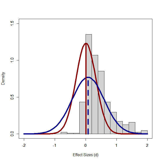
Figure 1 from Maier et al. (2024) shows the problem for the weight-function selection model underlying RoBMA. The distribution has a long positive tail that does not fit a single normal distribution (blue). A model that only fits the right side and attributes the low frequency of negative results to selection bias (red line). However, even this model does not fit the data well, but RoBMA has no other way to represent the data.
However, we can help RoBMA by removing extreme values from the data on both sides. However, because there are many more positive extreme values than negative extreme values, the exclusion of extreme values lowers the average of the observed data from 1.38 percentage points (pp) to 0.74 pp. In contrast, the median did not change much (0.50 vs. 0.42 pp).
Applying RoBMA to these data changed the estimate of the average effect size dramatically. The Bayes Factor now clearly rejected the nil hypothesis, BF > 14,999 (the maximum value in RoBMA). The estimated average was 0.58, only slightly lower than the simple average of 0.74 pp. This estimate also does not take the extreme positive results into account. The main point, however, is that RoBMA underestimated the average effect size when a long tail of positive results was included because it imagined a long tail of matching negative results based on the symmetry of the normal distribution. As Maier et al. (2024) already stated, this means RoBMA should not be used when data are likely to have a different distribution.
Maier et al. (2022) computed their RoBMA result ignoring the clustering of standard errors — as stated in their own figure caption. This is not a minor detail. The 448 effect sizes come from 212 studies, and treating dependent estimates as independent inflates the apparent precision that the bias correction then acts on. Without clustering, RoBMA returns a mean of essentially zero and evidence against an effect under every bias specification I tried — the full model-averaged ensemble, and a selection-model-only version with PET-PEESE removed (μ = 0.02, BF favoring the null). Once the clustering is modeled — using the multilevel extension of RoBMA (Bartoš, Maier & Wagenmakers, 2026) — the evidence reverses decisively (inclusion BF > 14,999) to a clearly positive mean, between d = 0.22 and d = 0.34 depending on the bias model. The published conclusion of “no evidence for nudging” is an artifact of ignoring the dependence structure of the data.
How Robust is RoBMA?
In statistics, robustness traditionally refers to methods that remain reliable when assumptions are violated or when data contain outliers or other atypical observations (e.g., Box, 1953; Huber, 1964; Tukey, 1960). Calling RoBMA “robust” may therefore give users the impression that it has these properties. However, robust in RoBMA refers primarily to averaging across a predefined set of meta-analytic models, not to robustness against misspecification of assumptions those models share. Bayesian model averaging can hedge against uncertainty about which model in the set is correct; it cannot protect against an assumption that every model in the set makes.
That distinction is important because RoBMA, like every statistical model, can produce misleading estimates when its assumptions are poorly suited to the data. In the present analyses, results depend strongly on assumptions about the distribution of population effect sizes and the treatment of extreme or highly heterogeneous effects. Other plausible models can produce substantially different conclusions.
The practical lesson is therefore that its results should not automatically be treated as the most robust or most credible estimate. When different models give different answers, the scientifically important task is to examine why they disagree and which assumptions are plausible for the data at hand.
Hu, B., Z. Xia, Q. Guo, C. Lu, S. Constantino, and X. Ju. 2025. “ Assessing Nudge Impact: A Comprehensive Second-Order Meta-Analysis.” Journal of Behavioral Decision Making 38, no. 5: e70053. https://doi.org/10.1002/bdm.70053.
Post-Publication Review
Hu et al. present a second-order meta-analysis of 14 meta-analyses covering 1,638 studies and nearly 30 million participants. They report an unadjusted mean effect of , while PET-PEESE reduces the estimate to approximately zero.
The main problem is that adding more and more studies does not solve the basic problem of extreme heterogeneity. The authors report , indicating that the included meta-analyses differ enormously in their estimated effects. Under these conditions, the question “What is the effect of nudging?” is not well defined. Defaults, reminders, food placement, information labels, and many other interventions are not repeated estimates of one common treatment effect.
The publication-bias results do not resolve this problem. In fact, they disagree. The conventional random-effects estimate is . RoBMA gives , 95% CI [.15, .43], with . Trim-and-fill still gives , and using adjusted estimates from component meta-analyses gives . Only PET-PEESE produces the near-zero estimate of –.004.
It is therefore misleading to foreground the PET-PEESE result as if different methods converge on zero. RoBMA already averages over PET-PEESE, selection, and no-bias models, yet its model-averaged estimate remains positive. Moreover, PET-PEESE relies on the relation between effect size and standard error, which can be confounded by genuine heterogeneity. In a literature where small and large studies differ in intervention type, setting, population, and outcome, that relation need not reflect publication bias alone. A separate weight-function estimate would have been informative, but none is reported.
More fundamentally, even a perfectly estimated grand mean would tell us little. The authors themselves show that effect sizes differ substantially across categories and domains; for example, decision-structure nudges have a descriptive estimate of , environmental nudges , and food nudges . Their moderator tests are underpowered and do not explain the heterogeneity, but failure to explain heterogeneity does not make the grand mean meaningful.
The article therefore does not tell us much that is new about nudging. We already knew that published effects are heterogeneous and that publication bias is a concern. Pooling ever larger numbers of heterogeneous studies does not answer the scientifically important questions: Which nudges work? How large are their effects? Under what conditions do they work?
The conclusion that the “true effect of nudging” is zero has the appearance of precision, but it is closer to answering an ill-defined question. The problem is not whether the grand mean is or . The problem is that there is no single effect of nudging to estimate.
Mertens, S., Herberz, M., Hahnel, U. J. J., & Brosch, T. (2022). The effectiveness of nudging: A meta-analysis of choice architecture interventions across behavioral domains. Proceedings of the National Academy of Sciences, 119(1), e2107346118. https://doi.org/10.1073/pnas.2107346118
Introduction
Hundreds of studies examined the effectiveness of nudging manipulations, and most of them reported a positive effect, often also a statistically significant one; that is, a result unlikely to be a statistical fluke. A 2022 meta-analysis included 447 effect sizes from 212 publications. The pooled meta-analytic estimate was—not 42, but 43; that is d = .43 or 43% of a standard deviation.
This answer is close to the famous answer to the question about the meaning of life, the universe, and everything else in The Hitchhiker’s Guide to the Galaxy, which was 42. The novel poked fun at the attempt to answer a complex question with a single number, but meta-analyses often do exactly this. The hundreds of studies in the nudging literature used different manipulations, different outcomes, and different populations. What is the probability that they all have the same effect size? Nil. So, the headline figure in a meta-analysis is at best the center of a heterogeneous distribution of effect sizes; it does not tell us the effect of any specific intervention.
This did not stop two research teams from reanalyzing the data with statistical methods designed to correct for publication bias and to produce another single number. This number was dramatically different. Szászi et al. (2022) used a step-function selection model and obtained an adjusted estimate of the average effect size of , with a very small standard error, . In other words, after bias correction, the average effect of nudging was now approximately zero.
A second commentary reported the results of another analysis using a new statistical method, Robust Bayesian Meta-Analysis (RoBMA), which averages across several models, including one similar to the model used by Szászi et al. (2022). The title of the article—which is the only thing many readers ever see—made the conclusion clear: “No evidence for nudging after adjusting for publication bias” (Maier et al., 2022). Their estimated average effect size, , was not exactly zero, but close enough to invite the interpretation that nudging effects are negligible or nonexistent.
There are several problems with both reanalyses that presented the average estimate as the key finding. The first one is that the average alone is meaningless, when the same model also estimates considerable heterogeneity around the average. Neither article reported the estimate of heterogeneity that the models produce, but a reanalysis of the data with the models shows considerable heterogeneity (weight-function model, sd = .5; RoBMA sd = .3). This implies that many positive effect sizes estimates were obtained with positive population effect sizes that can be replicated. Thus, the results do not imply that nudging never has an effect. At least sometimes, nudging had effects. This simple fact is easily conveyed by a figure that plots the predicted distributions of population effect sizes along with the distribution of observed effect sizes (Figure 1).
The histogram shows that 91% of the observed effect-size estimates are positive. In contrast, the fitted distributions of population effect sizes are centered close to zero and therefore imply nearly equal numbers of positive and negative true effects. How can models that imply so many negative effects fit data in which negative estimates are rare?
The answer lies in two assumptions built into the models. First, they assume that population effect sizes follow a normal distribution. The positive observed effects are concentrated near zero with a long right tail and therefore resemble the positive half of a normal distribution centered close to zero. Once the model places the center near zero, however, symmetry requires a corresponding negative half. Because this negative half is largely missing from the observed data, the discrepancy is attributed to selection: negative results are assumed to be observed, but remained unpublished.
But this is not the only explanation of the observed pattern. An alternative is that there really are relatively few negative population effects—that is, nudges usually have effects in the theoretically predicted direction—but that the distribution of positive effects is strongly non-normal. Most nudges may have effects close to zero, while a smaller number have moderate or large positive effects. Such a right-skewed distribution would also produce exactly what we see in the histogram: many small positive effects, relatively few negative effects, and a long positive tail.
The crucial point is that the models cannot distinguish these two explanations from the observed data alone. A symmetric distribution centered near zero combined with strong selection against negative results can resemble an asymmetric population distribution containing mostly positive effects and little or no selection against negative results. The near-zero mean therefore does not follow directly from the data. It follows from the assumption that the underlying distribution of population effects is approximately normal and symmetric.
Separating Positive and Negative Results
Fortunately, we do not have to decide which explanation is correct to learn something useful from these models. If all variation in observed effect sizes were merely sampling error around a single population effect, positive and negative estimates would have to be combined to estimate that common effect. But both models estimate substantial heterogeneity. In their own models, population effect sizes genuinely differ from one study to another.
We can therefore ask a different question. Rather than averaging positive and negative population effects into a single number, we can examine the two parts of the fitted distribution separately. In particular, we can ask: Among population effects that are in the theoretically predicted direction, what is their average magnitude? If desired, we could ask the corresponding question about effects in the opposite direction.
This is a different estimand from the grand mean. It is also important to distinguish it from simply averaging the 91% of observed estimates that are positive. Observed estimates contain sampling error, and some positive estimates may arise from population effects close to zero or even negative. Instead, we can use the models’ estimated normal distribution of population effect sizes to calculate the mean of the positive part of the normal distribution.
RoBMA’s estimate is d = .26, a small effect, but the step-function model produces an estimate of d = .44, very similar to the estimate of d = .43 in the original article that was based on all estimates. The mean of only positive results is d = .51, but it is reduced to d = .43 by the inclusion of the negative results.
In conclusion, the two critical reanalyses that reduced the estimated grand mean from about to approximately zero did not show that the positive effects themselves were reduced to zero after correcting for publication bias. In the step-function model, the estimated mean of positive population effects remains . Even RoBMA implies an average positive population effect of . The dramatic change in the grand mean arises largely because the models infer a substantial population of unobserved negative effects that counterbalances the positive effects.
Those missing negative effects may exist. Researchers may have obtained effects in the theoretically wrong direction and failed to publish them. But this does not imply that the positive effects are zero, nor does it show that their magnitudes were dramatically inflated. In particular, the step-function model provides little evidence that selection for statistical significance—the usual mechanism invoked to explain inflated published effect sizes—accounts for the observed pattern. Its strongest selection effect is for the direction of the effect: negative results are much less likely to appear.
This makes the presentation of the reanalyses misleading. The headline result was the grand mean close to zero, while the substantial heterogeneity around that mean was not reported in a way that made clear that the model implied a broad distribution of positive and negative effects. Nor was the weak evidence for selection at the conventional significance threshold emphasized. A very different headline could therefore have been: “Little evidence that selection for statistical significance inflated positive nudging effects.”
A Zcurve3 Analysis
Figure 1 also shows that neither model fits the distribution of positive results particularly well. RoBMA captures the concentration of weak effects near zero, but fails to reproduce the long tail of stronger positive effects. The weight-function selection model captures the positive tail better, but underestimates the large concentration of weak effects. Thus, estimates of the mean of the positive population effects remain sensitive to misspecification of the assumed normal distribution.
Zcurve3 provides an alternative approach because it does not assume that population effect sizes follow a normal distribution. Zcurve3 builds on zcurve 2.0 (Bartoš & Schimmack, 2022), but adds several features that are useful for the present analysis. First, it can model directional results while preserving the sign of an effect. By fitting the model only to positive effects, it can therefore examine the credibility and magnitude of effects in the theoretically predicted direction without making assumptions about a corresponding distribution of negative effects.
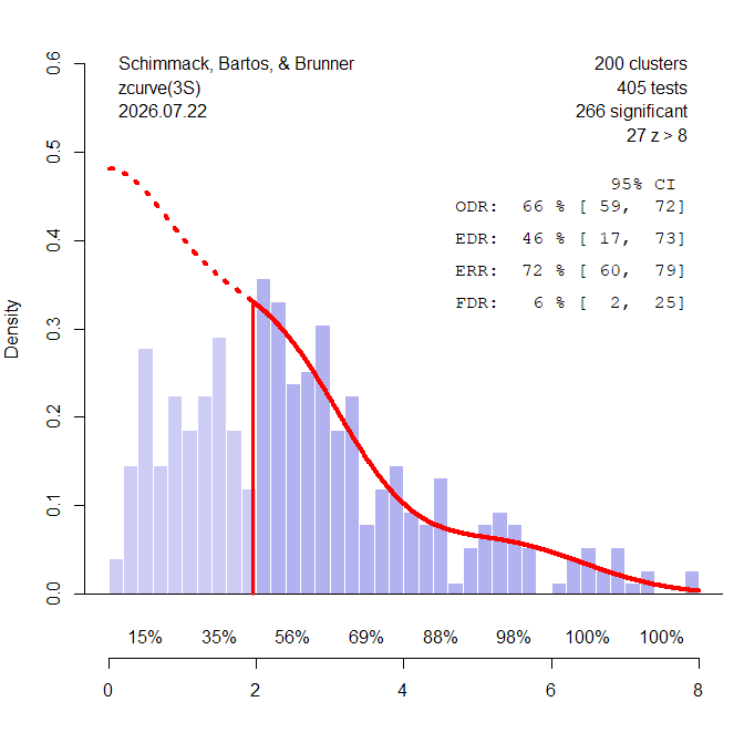
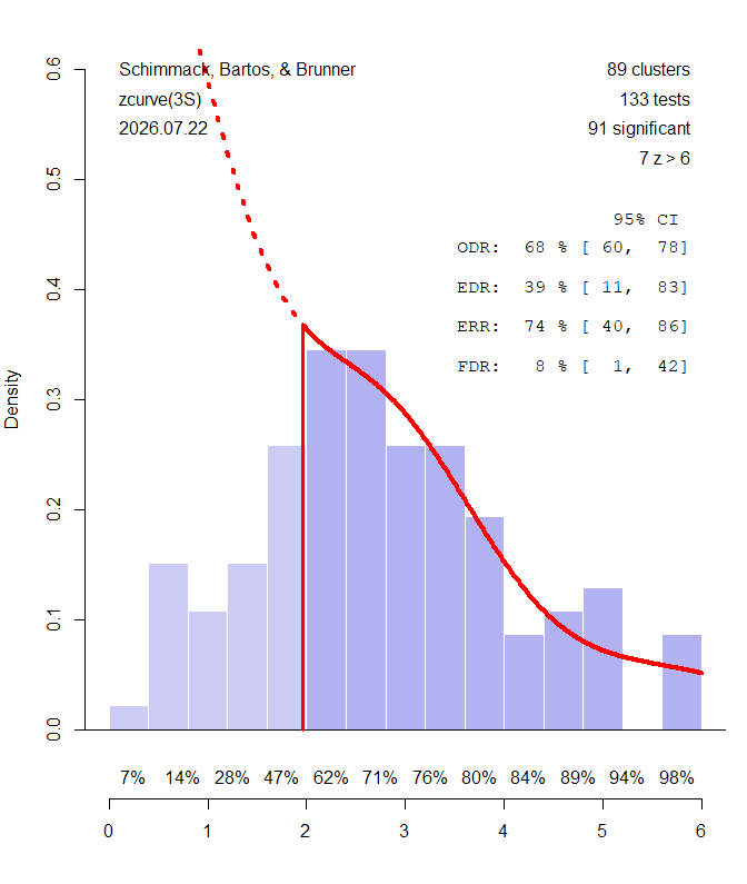
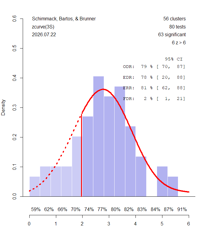
The plot confirms what the previous models suggested: there is no strong selection for statistical significance among the positive results. The observed discovery rate (ODR) is 66%, whereas zcurve3 estimates an expected discovery rate (EDR) of 46%. Thus, the point estimate suggests some selection for significance, but the confidence interval around the EDR is wide, ranging from 17% to 73%, and includes the observed rate of 66%. Consequently, the data do not provide clear evidence that non-significant results are missing. At the same time, the wide confidence interval means that substantial selection cannot be ruled out.
Zcurve3 also estimates a false discovery rate of only 6%, although the confidence interval is again wide, ranging from 2% to 25%. Thus, the results are inconsistent with an interpretation in which the large number of significant positive findings consists mostly of false positives. This is important because a grand mean close to zero can easily be misinterpreted as evidence that the significant nudging results have disappeared after correction for publication bias. That is not what these results show. They suggest that most significant results were obtained with a true effect.
Finally, zcurve3 estimates an expected replication rate (ERR) of 72%, 95% CI [60%, 79%]. This means that, under exact replication conditions, approximately seven out of ten significant positive results are expected to produce another significant result. Actual replication rates may be lower because replication studies are rarely exact and because effect sizes can vary across populations and contexts.
Replicability also increases sharply with the strength of the original evidence. The local-power estimates shown below the x-axis illustrate that studies with large z-values have a high probability of producing another significant result. Thus, even if the grand mean across all nudging interventions is close to zero, the literature clearly contains individual findings with substantial statistical evidence and high predicted replicability.
Zcurve3 also provides selection-adjusted effect-size estimates. For all positive results, the estimated mean effect is d = .37, 95% CI [.14, .60]. The confidence interval is wide because there is considerable uncertainty about how many nonsignificant positive results are missing and how small their effects are likely to be. Nevertheless, even the lower bound of the confidence interval is clearly above zero.
A statistically more precise estimate can be obtained for the significant positive results that are actually used to fit the z-curve model. Their estimated mean effect is , 95% CI [.47, .72]. This estimate answers a narrower question: what is the average effect size of the positive significant findings on which most published claims about successful nudges are based? For evaluating the credibility and magnitude of these claims, this conditional estimate is more informative than a grand mean that averages significant, nonsignificant, positive, and negative effects from fundamentally different interventions.
However, is still only an average. Considerable heterogeneity remains among these effects, , 95% CI [.13, .39]. Thus, I am not claiming that “the effect of nudging is .60.” There is no single effect of nudging. Zcurve3 provides a more meaningful average for a more narrowly defined question, but the remaining heterogeneity still needs to be examined. The next step is therefore not to replace 43 or 0 with 60 as the new answer to everything, but to identify which specific nudges produce credible effects and how large those effects are.
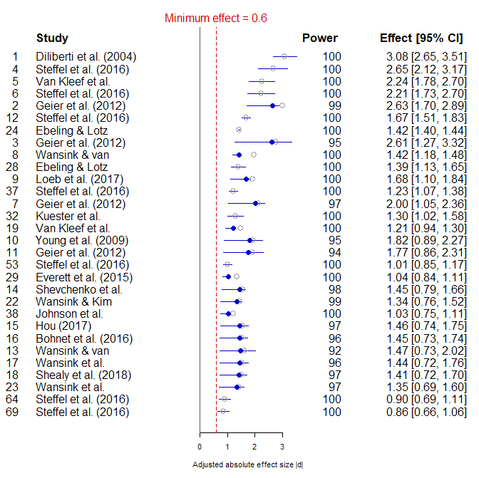
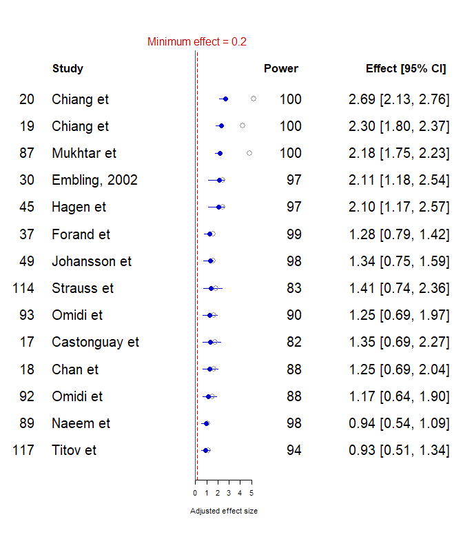
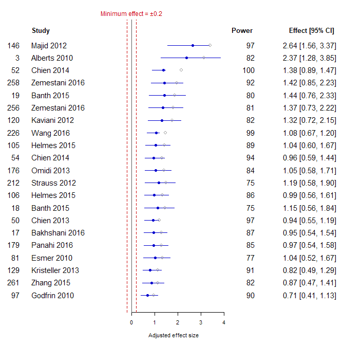
Zcurve3 provides a forest plot that makes it easy to identify particularly promising findings. The plot shows selection-adjusted effect-size estimates in blue, together with confidence intervals that incorporate both sampling error and uncertainty introduced by selection bias. Studies are ranked by the lower bound of their confidence interval rather than simply by their z-value or point estimate. Thus, studies rise to the top only when the data support an effect that is both reasonably large and estimated with sufficient precision. This avoids giving priority merely to very large studies that can produce impressive z-values for substantively trivial effects.
At the top of the forest plot is a study by Diliberti et al. (2004). Its z-value is outside the range used by Zcurve3 for effect-size adjustment, so the plot shows the reported effect size without correction. The estimate is , an enormous standardized effect. Even the lower bound of the confidence interval is . A result of this magnitude stands on its own and does not require a meta-analytic estimate. It deserves careful examination. However, an extreme meta-analytic effect-size estimate should never be trusted at face value. It could reflect a computational error in the original study, a coding error in the meta-analysis, or an unusual feature of the outcome measure. Closer inspection of the original article reveals why this estimate is so large.
Diliberti et al. manipulated portion size on different days in a cafeteria. On days when larger portions were served, customers ate more. The extraordinarily large standardized effect arose from the measure of entrée consumption. Customers who finished their entire entrée all received the same maximum value—the amount of food that had been served. This pile-up at the upper limit compressed the variance in consumption. Because a standardized effect size divides the mean difference by the standard deviation, an unusually small standard deviation can produce an extraordinarily large value of .
The article also reported total caloric intake for the entire meal, an outcome with substantially more variability. The absolute difference between conditions remained large, but the standardized effect was a much more plausible . Thus, the substantive finding is robust: larger portions increased food consumption. However, the estimate exaggerates the practical magnitude of the effect because of the unusually small variance in the outcome measure. It therefore contributes artificial heterogeneity to the meta-analysis—heterogeneity caused by the construction of the effect-size measure rather than by a substantively stronger effect of the intervention. No continuous theoretical moderator of nudging should be expected to explain such an extreme value.
Once the source of an extreme effect size has been identified, it is reasonable either to replace it with a more appropriate effect-size estimate or to exclude it in a sensitivity analysis when estimating the remaining unexplained heterogeneity. This is different from deleting an outlier simply because it is extreme. The reason for treating this value differently is known: is inflated by restricted variance in the particular outcome that was selected to represent the study.
Another question is whether a portion-size manipulation should be included in a meta-analysis of nudging in the first place. Maier et al. (2022) tried to address heterogeneity by conducting separate analyses for six broad domains. For the food domain, the Bayes factor favored a nonzero average effect, although the evidence was weak. In the other five domains, the Bayes factors pointed toward a mean of zero to varying degrees (), although only three reached the conventional 3:1 threshold for moderate evidence. Nevertheless, these results have been summarized as showing that “using more precise estimates, the results revealed evidence against the efficacy of nudges in most domains” (PsyPost). This statement illustrates how easily results from RoBMA can be misinterpreted. A Bayes factor concerns the average effect within a domain. Even a Bayes factor of 1000:1 in favor of a mean of zero would not show that nudges have no effects when the same model estimates substantial heterogeneity. Thus, all reported means should be reported with the estimate of heterogeneity to avoid this misinterpretation.
Maybe the old criticism that heterogeneous meta-analyses compare apples and oranges was right after all (Sharpe, 1997). If apple studies and orange studies have systematically different effect sizes, their average is informative about neither apples nor oranges. Combining them merely creates heterogeneity. When a moderator analysis eventually discovers the apple-orange distinction, researchers report separate estimates for apples and oranges. But they could have done that from the beginning, without first mixing them together and reporting an average effect of “fruit.”
Another question is whether a portion-size manipulation should be included in a meta-analysis of nudging in the first place. Maier et al. (2022) also examined six different domains and found support for an average effect in the food domain. However, their Bayesian statistic pointed towards evidence for the null hypothesis to various degrees (BF01 > 1) in five other domains. This finding has been reported as “using more precise estimates, the results revealed evidence against the efficacy of nudges in most domains” (psypost.org). This claims illustrates how confusing RoBMA results can be and how they are easily misunderstood. Most importantly, even a Bayes-Factor of 1000:1 in favor of a mean of zero in these analysis does not justify the claim that there is no effect when studies also show heterogeneity.
Maybe the old criticism that heterogeneous meta-analyses are like comparisons of apples and oranges was right after all (Sharpe, 1997). If apple studies and orange studies have systematically different effect sizes, their average is informative about neither apples nor oranges. Combining them merely creates heterogeneity. When a moderator analysis eventually discovers the apple-orange distinction, researchers report separate estimates for apples and oranges. But they could have done that from the beginning, without first mixing them together and reporting an average effect of “fruit.”Maybe the old criticism that heterogeneous meta-analyses are like comparisons of apples and oranges was right after all (Sharpe, 1997). If apple studies and orange studies have systematically different effect sizes, their average is informative about neither apples nor oranges. Combining them merely creates heterogeneity. When a moderator analysis eventually discovers the apple-orange distinction, researchers report separate estimates for apples and oranges. But they could have done that from the beginning, without first mixing them together and reporting an average effect of “fruit.”
This points to an even more fundamental problem with averaging positive and negative population effects. Suppose eating an apple a day keeps the doctor away, whereas eating an orange a day makes people sick. Both are real effects. They receive positive or negative signs only because of a convention about which direction is desirable or consistent with a theoretical prediction. If the two effects are equal in magnitude but opposite in sign, their average is zero. But this does not imply that there is no effect. It implies that two real effects cancel mathematically when they are averaged. The scientifically useful conclusion would be to eat apples and avoid oranges—not that “fruit has no effect.”
Meta-analyses in medicine often take a much narrower approach. Rather than combining fundamentally different treatments and outcomes under a broad label, they typically focus on closely related interventions, comparable control conditions, similar populations, and clearly defined outcomes. As a result, many clinically informative meta-analyses contain fewer than 20 studies. That may sound less impressive than a meta-analysis based on more than 200 publications, but in meta-analysis, more is not necessarily better. Often, less is more—except when it comes to the sample sizes of the original studies. A meta-analysis gains credibility from the comparability of the studies, not from the sheer number of papers thrown into it.
The broader lesson is that methods designed to evaluate the credibility of published research must themselves be evaluated critically. Meta-scientists are subject to the same incentives as other scientists, and sophisticated statistical methods do not eliminate the need to examine assumptions, alternative explanations, and the full implications of a fitted model. In this case, focusing on a grand mean close to zero obscured substantial heterogeneity, little evidence of selection for statistical significance, and considerable evidence for positive and potentially replicable effects. A credibility revolution should make scientific claims more carefully calibrated, not merely replace one headline number with another.
Selected References
Bartoš, F., & Schimmack, U. (2022). Z-curve 2.0: Estimating replication rates and discovery rates. Meta-Psychology, 6, Article e0000130. https://doi.org/10.15626/MP.2022.2981
Maier, M., Bartoš, F., Stanley, T. D., Shanks, D. R., Harris, A. J. L., & Wagenmakers, E.-J. (2022). No evidence for nudging after adjusting for publication bias. Proceedings of the National Academy of Sciences, 119(31), e2200300119. https://doi.org/10.1073/pnas.2200300119
Sharpe D. (1997). Of apples and oranges, file drawers and garbage: why validity issues in meta-analysis will not go away. Clinical psychology review, 17(8), 881–901. https://doi.org/10.1016/s0272-7358(97)00056-1
Szászi, B., Higney, A., Charlton, A., Gelman, A., Ziano, I., Aczel, B., Goldstein, D. G., Yeager, D. S., & Tipton, E. (2022). No reason to expect large and consistent effects of nudge interventions. Proceedings of the National Academy of Sciences, 119(31), e2200732119. https://doi.org/10.1073/pnas.2200732119
A RoBMA estimate near zero is not, by itself, evidence that there is no effect. It is a model-averaged posterior estimate that can be pulled toward zero by the prior for the effect under and then pulled toward zero again by posterior weight on the point-null model. Therefore, a RoBMA estimate near zero does not imply that the true average effect is zero, or even close to zero.
Moreover, if RoBMA also finds substantial heterogeneity, even a true average effect of zero should not be interpreted as evidence that “there is no effect.” It means only that positive and negative population effects balance so that their average is zero. Individual effects may still be substantial. Thus, the point-null hypothesis for the mean is not equivalent to a no-effect hypothesis when effects are heterogeneous.
Finally, model averaging does not guarantee that the resulting average is closer to the truth. It averages estimates from models according to their posterior weights, but all of those models may rely on incorrect or weakly identified assumptions. It is therefore important to examine the estimates from the individual models, the conditional estimate under , the posterior evidence for heterogeneity, and the sensitivity of the result to alternative prior specifications rather than interpreting the model-averaged estimate alone.
Introduction
Psychology has been trying for decades to become a real science. However, the replication crisis in social psychology has revealed that the scientific practices of empirical psychologists produce many results that cannot be replicated in later studies (Open Science Collaboration, 2015). The realization that published results are not as robust as they appear has been called the credibility crisis. In response to the credibility crisis, methodologists and meta-psychologists have debated the causes of replication failures and proposed solutions to the credibility crisis.
Some suggestions have produced real change that increases credibility. Personally, I would argue that the sharing of data has been the biggest positive change. Before, researchers would state that data are available on request, but requests often resulted in apologies why the data could not be shared (my dog ate my USB stick). Now it is expected and sometimes even requested by journals that data are shared openly. That makes it possible to find errors in the statistical analyses and occasionally even evidence of data tampering. However, when open data reproduce the original result, it still remains unclear what the data tell us about a particular hypothesis or theory. The reason is more complex and rooted in the problem that many psychological effects are weak and that studies often have large amounts of sampling error. Sampling error simply means that random factors influence the results and a new sample would produce different results. Although this problem is not new or specific to psychology, it remains unsolved. That is, the same data can be analyzed with methods that produce different answers. One method may conclude that the data support a hypothesis and another one leads to the opposite conclusion. The main problem is that empirical researchers often lack the training (and motivation) to understand why different methods produce different results.
Nil Hypothesis Testing Is Wrong
The reason why different models produce different results with the same data is that they make different assumptions about the data and that they answer different questions. The problem is that researchers have a simple question (e.g., how much does listening to music during studying decrease test performance,” but there is no simple way to answer this question. Statistical methods answer questions that can be answered and researchers then report these answers as if they answered the actual question.
This indirect approach of drawing inferences from data is enshrined in the nil-hypothesis ritual that still dominates psychology. After allocating students to a condition with music or no music, the means are compared and the sampling error (standard error) is computed. The ratio of the two is used as a measure of how compatible the data are with the nil hypothesis that there is absolutely no difference. Exactly zero, zip, nada. If the test statistic is above a conventional criterion value, the nil hypothesis is rejected in favor of the conclusion “Music influences learning!” This ritual has been criticized more often than anybody can count and it doesn’t even tell us whether music increases of decreases performance. It just says, the effect is not nil (zero). Let’s say, the sign is negative. However, we still do not know how much music decreases performance. Maybe it changes a grade by 1 percentage point, maybe it is 10 percentage points. So, the answer to the question “How much does music decrease performance” is “It is not zero.” The answer is correct, but not the answer we wanted.
Even worse, the answer could be false. Psychologists use a criterion value that produces a false positive result in 5% of all tests in which the nil hypothesis is true; the effect is really exactly zero. An error rate of 5% may seem low, but this does not mean that only 5% of the results reported in textbooks are false. The reason is that textbooks focus on the studies that rejected the nil hypothesis for a good reason. The other studies are simply inconclusive and do not tell us anything about direction or strength of an effect, if we use this statistical approach.
If results are selected because they showed an effect, it remains possible that all of the published results are false rejections of a hypothesis. This is not just a hypothetical concern. Some people have argued that published studies report more false results than true results.
In conclusion, the most widely used statistical approach in empirical psychology makes it possible that most published results are false, and the replication crisis suggested that false positives contribute considerably to replication failures.
Bayesian Salvation?
The credibility crisis created an opportunity for Bayesian statisticians who had long criticized nil-hypothesis significance testing. One attraction of Bayesian hypothesis testing is that it promises something conventional significance testing cannot provide: evidence in favor of the nil hypothesis. A nonsignificant -value does not tell us that the nil hypothesis is true. A Bayes factor, in contrast, can compare a model in which the effect is exactly zero with a model in which the effect can take other values.
This sounds like progress. If psychologists have produced too many false positive results, a method that can distinguish evidence for an effect from evidence for no effect seems useful. The problem is that the ability to produce evidence for the nil hypothesis does not guarantee that the evidence is correct. Just as significance testing can falsely reject a true nil hypothesis, Bayesian hypothesis testing can favor a false nil hypothesis.
Whether this happens depends on the assumptions built into the Bayesian models and their priors.
The Problem of Priors
Bayesian statisticians are aware that prior assumptions influence their results, and they are usually explicit about this. However, the terminology can be misleading to users who are not Bayesian statisticians. Some priors are described as “objective” priors. In everyday language, objective sounds as if the prior is neutral and does not influence the result. That is not what the term means.
An objective prior is better understood as a conventional prior that was chosen without considering the specific subject matter. In this sense, it is similar to using an alpha level of .05 in significance testing. Researchers do not choose .05 because there is something special about their particular hypothesis that makes .05 appropriate. They use it because it has become a convention. Likewise, an objective prior is typically based on a general rule that can be applied across many different research questions.
But standardized does not mean neutral. The prior is still an assumption, and it can influence the result. Different priors applied to the same data can produce different posterior estimates and different conclusions. There is nothing mathematically wrong with this. It is an intended feature of Bayesian statistics. The problem arises when results are presented as if they were produced by the data alone.
A Bayesian result is always conditional on both the data and the prior assumptions used to interpret them. Thus, “objective” does not mean “assumption-free.” It means that the assumption was chosen by a general convention rather than by considering the particular phenomenon being studied.
This is similar to other potentially misleading terms in statistics. “Statistically significant” does not mean that an effect is important. In the same way, an “objective prior” does not mean that the prior has no influence on the result. The technical meaning may be clear to statisticians, while the everyday meaning encourages users to infer more than the term actually implies.
The criticism developed here is therefore not a criticism of Bayesian statistics in general. Bayesian statistics allows researchers to use many different priors, including priors informed by substantive knowledge. The concern is what happens when conventional priors are used without considering whether they make sense for the research question at hand.
One particularly important choice is whether one specific value should receive special prior probability. In Bayesian hypothesis testing, that value is often zero. A model in which the effect is exactly zero is compared with a model in which the effect can take a range of other values. This makes it possible to do something that conventional significance testing cannot do: provide evidence in favor of a nil hypothesis.
That sounds like an important improvement. A nonsignificant p-value does not provide evidence that the effect is zero, whereas a Bayes factor can favor a model in which the effect is fixed at zero.
But this advantage creates the possibility of the opposite error. Conventional significance testing can falsely reject a true nil hypothesis. Bayesian hypothesis testing can favor the nil hypothesis when the true effect is not zero.
Suppose, for example, that psychotherapy has a small positive average benefit. A Bayesian analysis could nevertheless favor a model in which the average effect is exactly zero. The calculation may be mathematically correct, while the conclusion is wrong because the prior and model assumptions were poorly suited to the problem.
Before the credibility crisis, psychologists were highly concerned about low statistical power and failures to detect real effects (Cohen, 1994). More recently, attention has shifted heavily toward false positive results. Both types of error matter. A method that reduces false positives by substantially increasing the risk of falsely concluding that real effects are absent is not necessarily an improvement.
The important question is therefore not whether Bayesian statistics is better or worse than conventional significance testing. The important question is how strongly the conclusion depends on the prior assumptions that were chosen and whether those assumptions make sense for the research question.
This issue becomes especially important for Robust Bayesian Meta-Analysis because its default analysis gives zero a privileged role in more than one way.
Meta-Analysis
Disagreement among statisticians often focuses on the problem of drawing conclusions from a single study. How much did racism and sexism influence the outcome of the 2024 U.S. presidential election? A single study cannot provide a definitive answer, and we cannot repeat the election under identical conditions.
Psychologists are often in a better position because many of the effects they study can be examined repeatedly. Does psychotherapy work? This question has been studied for decades and will continue to be studied. So, it may seem that we can simply combine the results of all available studies in a meta-analysis and get a better answer.
Unfortunately, combining many studies is not as simple as it sounds.
The first problem is that effects vary. Psychotherapy may work differently for different disorders, treatments, populations, therapists, and circumstances. There is therefore no single effect size that describes every situation. At best, a meta-analysis can estimate the average effect and how much effects vary around that average.
The second problem is publication bias. Studies with positive or statistically significant results are more likely to be published than studies with negative or inconclusive results. As a result, the published literature can give an exaggerated impression of the average effect.
This problem was largely ignored for many years, and traditional meta-analyses sometimes produced inflated effect-size estimates, including apparently impressive evidence for implausible phenomena such as extrasensory perception. In response, statisticians have developed a variety of methods that try to detect publication bias and estimate what the average effect might have been if all studies had been available.
Unfortunately, this is a difficult problem. Simulation studies show that publication bias can be hard to detect, especially when it is modest. More importantly, different correction methods can produce very different answers from the same data. One method may estimate an average effect of zero, while another estimates an effect of .20.
The reason is that the methods make different assumptions about how studies came to be published and about the distribution of the missing results. When those assumptions are approximately correct, a method may recover the true effect reasonably well. When they are wrong, the estimate can be badly biased.
The crucial difficulty is that the missing studies are, by definition, missing. The observed data often contain too little information to determine which assumptions about the missing results are correct. Consequently, publication-bias adjustments are not simply estimates produced by the data. They are estimates produced by the data plus assumptions about the data we do not see.
Properly interpreted, the results are therefore conditional: “If the assumptions of Model A are approximately correct, the average effect is close to zero. If the assumptions of Model B are approximately correct, the average effect is closer to .20.
Robust Bayesian Meta Analysis (RoBMA)
Robust Bayesian Model Averaging (RoBMA) offers a solution to the problem that different meta-analytic models can produce different answers. RoBMA fits many models to the same data, gives more weight to models that receive more support from the data, and then averages estimates across these models.
However, RoBMA can move estimates toward zero in two different ways. First, even models that allow for a nonzero average effect use a prior distribution for the size of that effect. When the data provide weak information, this prior can pull the conditional estimate toward its prior mean. For example, a true average effect of .20 might produce a conditional estimate of only .10 if the prior favors smaller effects.
Second, RoBMA also includes models in which the average effect is fixed at exactly zero. When RoBMA remains uncertain about whether the average effect is zero or nonzero, these models receive posterior weight in the final average. If the conditional estimate from the nonzero-effect models is .10 and the zero and nonzero models receive roughly equal weight, the final model-averaged estimate will be approximately .05.
Thus, a true average effect of .20 can first be reduced to .10 by the prior within the nonzero-effect models and then reduced again to .05 by averaging this estimate with models that fix the average at zero. Both steps are mathematically legitimate Bayesian operations. But neither step guarantees that the estimate is moving closer to the true value.
This procedure produces a single number, but it does not make disagreement among the models disappear. If one plausible model produces an estimate near zero and another produces an estimate near .20, this disagreement tells us that the answer depends strongly on assumptions. Averaging the estimates does not resolve that problem. Adding further weight to models that fix the average at zero may move the final estimate closer to zero, but there is no reason why closer to zero must mean closer to the truth.
RoBMA therefore does not eliminate the uncertainty created by conflicting models. It summarizes this uncertainty by averaging across them. The danger is that users may interpret the resulting single estimate as if the disagreement had been resolved. In some situations, the disagreement among individual models is more informative than their average because it reveals how strongly the conclusion depends on assumptions.
Default RoBMA
Default RoBMA gives zero a privileged role in two different ways.
The first prior concerns the size of the average effect when an effect is assumed to exist. RoBMA specifies a distribution of plausible effect sizes, and the default distribution is centered at zero. Before seeing the data, small effects are therefore considered more plausible than large effects, with positive and negative effects treated symmetrically. When the data contain strong information about the average effect, this prior has little influence. When the data contain weak information, however, the estimate remains closer to the center of the prior. Thus, even conditional on the assumption that there is an effect, the default prior can move the estimated effect toward zero.
There is nothing inherently Bayesian about centering this prior at zero. A researcher could specify a prior centered at .10, .20, or some other value. The default of zero is a conventional choice made without substantive information about the particular phenomenon being studied. It may be reasonable in some applications, but it is not neutral: changing the center of the prior can change the estimate when the data are weakly informative.
The second prior gives zero an even more privileged role. RoBMA distinguishes between models in which the average effect is estimated and models in which the average effect is fixed at exactly zero. By default, these two possibilities receive equal prior probability.
A 50:50 split can appear neutral because there are two hypotheses and each receives half of the prior probability. But this appearance is misleading. Zero is only one possible value of the average effect. There is no mathematical reason why exactly zero rather than .01, -.01, or .10 should receive a special probability of 50%. We could construct the same Bayesian model with a spike at .10 and give that value half of the prior probability. The resulting model would then be pulled toward .10 rather than toward zero. Bayesian mathematics permits either choice. The reason for privileging zero must therefore come from the substantive interpretation of zero, not from probability theory itself.
One justification for giving zero special status is parsimony. This makes sense for some statistical problems. If a regression coefficient is exactly zero, the corresponding predictor can be removed from the model. The zero coefficient therefore represents a genuinely simpler model: the predictor does not matter.
This logic is much less convincing for the average of heterogeneous effects in a meta-analysis. If some effects are positive and others are negative, an average of zero does not mean that nothing is happening. It merely means that the positive and negative effects cancel on average. Treating this as a no-effect model would be like calculating the average regression coefficient across many predictors, finding that the positive and negative coefficients average to zero, and concluding that all of the predictors can be ignored.
Thus, even if a point mass at zero can be justified for a single effect or a single predictor, the same parsimony argument does not automatically justify giving special status to a zero average when the individual effects vary.
Nor is there empirical evidence that the average effects studied in psychology have a 50% probability of being exactly zero. The 1:1 prior is a conventional default, not an empirical estimate of how often nil hypotheses are true. Other prior probabilities can be chosen, but there is no generally accepted value that follows from the data themselves.
More importantly, a prior probability for the nil hypothesis is not needed simply to estimate the average effect size. It is needed because RoBMA also asks a categorical question: should the data be attributed to a model in which the average effect is exactly zero or to models in which the average effect is allowed to differ from zero?
These are different questions. Researchers may want to know whether the data discriminate between a point-null model and an alternative model. But the usual goal of a meta-analysis is more straightforward: What is the best estimate of the average effect, and how uncertain is that estimate?
The distinction matters because the answer to the categorical question feeds back into the reported model-averaged effect size. If RoBMA remains uncertain about whether the average is exactly zero, posterior probability remains on the zero model. The conditional estimate from the models that allow an effect is then averaged with zero. Consequently, uncertainty about whether the nil hypothesis is true becomes additional shrinkage of the estimated effect toward zero.
This means that two different prior assumptions can work together. The prior for the size of the effect can pull the conditional estimate toward zero, and the prior probability assigned to the point-null model can then pull the model-averaged estimate toward zero again.
Neither operation is mathematically incorrect. But neither guarantees movement toward the truth.
A Simulation Example
Many meta-analyses in psychology show small average effects together with substantial heterogeneity (van Erp et al., 2017). I used a simple simulation to examine whether RoBMA can produce false evidence for the nil hypothesis under these conditions.
True effect sizes were drawn from a normal distribution with an average effect of and a standard deviation of .40. Thus, the true average effect was clearly nonzero, but individual effects varied widely and could be either positive or negative.
Rather than simulating particular sample sizes, I simulated the standard error of each study directly from a uniform distribution ranging from .05 to .30. True effect sizes and standard errors were independent.
This setup deliberately satisfied two important assumptions of models included in RoBMA. First, true effect sizes followed a normal distribution, which is the population distribution assumed by the random-effects selection models. Second, true effect sizes were independent of their standard errors, so there was no genuine small-study effect of the kind modeled by PET and PEESE.
Publication bias was introduced in a particularly simple way. Only studies with positive observed effect sizes were retained. There was no additional selection for statistical significance and no p-hacking. Selection depended only on the direction of the observed effect.
This form of publication bias is directly relevant to RoBMA because its step-function selection models can include a cutoff at , allowing studies with effects in one direction to have different publication probabilities from studies with effects in the opposite direction. Thus, the simulation did not confront RoBMA with a form of selection that lies outside the model space.
Ironically, the model designed to handle directional selection is central to the problem examined here. Given a normal distribution of heterogeneous effects, an observed literature containing only positive results implies that negative results are missing. RoBMA therefore has to reconstruct the unseen negative part of the distribution.
The difficulty is that the observed positive studies do not uniquely determine where the center of the complete distribution lies. A population centered at .20 with substantial heterogeneity and many missing negative results can generate the observed data. But a population centered much closer to zero, combined with a somewhat different amount of directional selection, can also fit the observed positive tail. Because RoBMA includes models that fix the average effect at zero and gives these models positive prior weight, this ambiguity can move the model-averaged estimate toward zero even when the true average is .20.
This is the key identification problem. The data contain a great deal of information about the studies that were observed, but much less information about the studies that were not observed. As a result, RoBMA can remain uncertain about the true average even when hundreds of studies are available.
That uncertainty creates room for the priors to matter. The prior under the alternative hypothesis can pull the conditional estimate toward its own center, and the separate point-null prior can then pull the model-averaged estimate toward zero again.
The simulation is therefore intentionally favorable to RoBMA in several respects. The true effect distribution is normal, there is no relationship between true effect sizes and standard errors, there is no p-hacking, and the publication process consists of simple directional selection that RoBMA explicitly allows for. Nothing in this setup would lead an applied researcher to expect that default RoBMA should frequently provide evidence for an average effect of exactly zero when the true average effect is .
Simulation Results
Across 100 simulations, the average RoBMA estimate of the average effect size was only d = .065, although the true average was . All credible intervals included zero, whereas only 81% included the true value of .20. Thus, the intervals consistently treated zero as plausible, while failing to include the true effect in 19% of the simulations. The uncertainty intervals therefore do not provide convincing evidence for the true effect and are clearly shifted toward zero.
RoBMA also reports Bayes factors that compare models in which the average effect is exactly zero with models in which it is not. Bayes factors are continuous measures of evidence and do not require a decision to accept or reject the nil hypothesis. In practice, however, conventional cutoffs are often used to describe evidence as favoring one hypothesis or the other. A Bayes factor greater than 3 is commonly interpreted as moderate evidence.
Using this criterion, RoBMA found moderate evidence for a real average effect in only 6% of the simulations. More importantly, it found moderate evidence for the false hypothesis that the average effect was exactly zero in 31% of the simulations. Thus, RoBMA did more than remain uncertain about a small true effect. In about one third of the simulations, it provided evidence in the wrong direction.
RoBMA can also report a conditional estimate that excludes models in which the average effect is fixed at zero. Across simulations, this conditional estimate averaged d = .130. Thus, even within models that assume an effect exists, the estimate had already been pulled substantially from the true value of .20 toward zero.
The default model-averaged estimate was still lower, because RoBMA further down-weights the conditional estimate according to the posterior probability that an effect exists. On average, this posterior probability was only about 40%, below its prior value of 50%. The average model-averaged estimate is not simply , because the conditional estimate and posterior probability vary together across simulations. Nevertheless, the mechanism is clear: substantial posterior probability remains on models that fix the average effect at exactly zero, and these models contribute zero to the final average.
The estimate is therefore moved toward zero twice. First, within models that allow an effect, the true average of .20 is reduced to a conditional estimate of .126. Second, averaging these estimates with models that fix the effect at zero reduces the final reported estimate further, to .064.
The different model families reveal an additional problem. When RoBMA is restricted to the step-function selection models, it reproduces the near-zero estimate. When it is restricted to PET/PEESE regression models, however, it produces an estimate of approximately .
At first sight, the PET/PEESE estimate may appear to be a severe overestimate because the true average across all effects is .20. But PET/PEESE does not model selection by direction. It only adjusts for the part of the observed effect that is associated with standard error—the small-study-effect pattern that often results from selective publication of statistically significant findings.
In this simulation, selection was based on direction rather than significance: only positive observed effects were retained. This selection induced only a small correlation between effect size and standard error, about . The mean observed effect among the selected studies was approximately , whereas the mean true effect among those selected studies was approximately . PET/PEESE detected the small association with standard error and reduced the estimate slightly, from .44 to .42. Thus, under this selection mechanism, PET/PEESE effectively estimates the average effect among the surviving positive studies rather than reconstructing the mean of the complete population.
The contrast between the model families is therefore striking. The step-function models produce an estimate close to zero, whereas PET/PEESE produces an estimate around .42. These are not simply two noisy estimates of the same quantity. They reflect fundamentally different assumptions about what happened to the missing studies and, in this simulation, effectively refer to different quantities.
Ironically, an equal arithmetic average of the step-function estimate of about .06 and the PET/PEESE estimate of about .42 would be approximately .24, close to the true value of .20. But this would be an accident, not a meaningful solution. Nobody is interested in the average of the mean across all effects and the mean among only the positive effects.
RoBMA did not average these two estimates equally. It assigned essentially zero weight to the PET/PEESE models and therefore reported an estimate dominated by the step-function models. The fact that this estimate happened to be much farther from the truth than the PET/PEESE estimate illustrates an important limitation of model averaging: giving more weight to one model does not guarantee that its estimate is closer to the true value.
In sum, this example demonstrates two distinct problems. First, RoBMA can provide evidence that the average effect is exactly zero when the true average is a small positive effect. Second, averaging across models with different assumptions does not guarantee a more accurate or even a more meaningful estimate. In this case, the disagreement between estimates of approximately .06 and .42 is itself important information. It reveals how strongly the answer depends on assumptions about the missing studies. Averaging that disagreement away does not resolve the uncertainty.
Alternative Solution: Mindful Meta-Analysis
RoBMA was developed to address a real problem: different methods for correcting publication bias can produce dramatically different answers from the same data. This blog post shows why automatically averaging these answers does not solve the problem. The models disagree because they make fundamentally different assumptions about how the observed data were generated and about the results that were not observed. Combining their estimates into a single number does not resolve these disagreements. It can merely hide them behind an algorithmic average.
This is similar to the problem Gigerenzer identified in the ritualistic use of nil-hypothesis significance testing. The problem was not the mathematics of significance testing. It was the replacement of scientific reasoning by an automatic procedure: calculate a p-value, compare it with .05, and report the appropriate conclusion. Replacing this ritual with another automatic procedure—fit many Bayesian models, average them, and report one number—does not solve the fundamental problem. Data analysis requires researchers to think about what their models assume and what question they are trying to answer.
In this example, asking about the true average for a hypothetical population of effect sizes that includes negative values when only positive values are observed is the wrong question. The same positive distribution could arise in a fundamentally different way. Imagine that effects were generated directly from a distribution that contained only positive values. No negative results would have been suppressed because no negative effects ever existed. The observed data could look essentially the same, but reconstructing a large number of hypothetical negative results would now be wrong.
This is the fundamental identification problem. From the observed positive results alone, the model cannot know whether negative results once existed and were suppressed or whether the population that generated the data simply contained few or no negative effects. The answer comes from assumptions about the missing part of the distribution, not from direct observation.
In this specific case, a more meaningful question is whether the positive observed results all tested a true nil hypothesis, which is already rejected by the large estimate of heterogeneity that implies at least some of the positive results were obtained with real effects. In this case, the PET-PEESE estimate actually provided the correct answer about the average effect size of the observed results. In contrast, users who focus on the average estimate of RoBMA might arrive at the false conclusion that the true effect size is zero, which ignores the evidence of heterogeneity. When studies are heterogeneous, there is no single effect size to estimate. Thus, even the misleading estimate of zero would require further examination of the positive results as a next step.
In conclusion, meta-analysis requires a lot more thinking than published meta-analyses that focus on the average effect size estimate imply. The devil is not only in the defaults of meta-analytic models, it is also hidden in large estimates of heterogeneity that remains unexplained. If mindless use of p-values got us into the mess, mindless use of Bayesian model averages is not going to get us out of it.
Conclusion: A meta-analysis of clinical trials in Western nations that compare psychotherapy to treatment as usual shows an average effect size of half a standard deviation with 95% of effects ranging from a quarter to three-quarters of a standard deviation. Thus, psychotherapy is an important component of treatment for depression.
Introduction
Psychotherapy works, .
However, a statistically significant result alone does not really help practitioners and patients assess the benefits of psychotherapy. The important question is not “Is the effect greater than zero?” but “How much does psychotherapy help?”
A single study cannot answer this question precisely because psychotherapy studies tend to have relatively small samples and therefore substantial sampling error. Meta-analysis was developed to address this problem. A simple meta-analysis combines the effect-size estimates from individual studies while taking their sampling error (standard errors) into account to obtain a more precise estimate of the average effect. As the number of studies increases, sampling error in the average estimate can become practically negligible.
The headline estimate of psychotherapy effectiveness is about 70% of a standard deviation on a measure of clinical depression such as the Beck Depression Inventory (), with very little sampling error (; Plessen et al., 2023). This suggests that psychotherapy has a substantial positive effect. However, although the average effect can be estimated very precisely, two other sources of uncertainty undermine the usefulness of this estimate: (a) publication bias and (b) variation in true effect sizes across populations, treatments, control conditions, and other study characteristics.
Publication Bias
One problem is publication bias. Studies that show that psychotherapy is effective may be more likely to be published than studies that fail to show an effect. If so, the published literature will exaggerate effectiveness. Plessen et al. (2023) therefore included PET–PEESE, a statistical method designed to estimate the effect after accounting for a possible relationship between effect size and sampling error.
The method exploits the fact that small studies need larger estimated effects to achieve statistical significance, whereas large studies can achieve significance with smaller estimated effects. If statistically significant findings are preferentially published, this creates a relationship between sampling error and observed effect sizes. PET–PEESE uses this relationship to estimate what the effect would be as sampling error approaches zero. Across the PET–PEESE analyses in Plessen et al.’s multiverse, the estimated effect averaged only .
The problem is that publication bias is not the only reason why effect sizes might be related to study size. Small and large studies may differ systematically in other ways. For example, smaller studies might provide more intensive and costly treatments, whereas larger trials might use briefer or online interventions. Control groups, patient populations, and other study characteristics may also differ with study size. If these characteristics genuinely influence treatment effects, PET–PEESE can mistake real differences in treatment effectiveness for publication bias and adjust the effect downward too strongly.
We are therefore left with remarkably different answers to a seemingly simple question. A conventional meta-analysis suggests an effect of , whereas PET–PEESE suggests an effect closer to . Is psychotherapy highly effective, only modestly effective, or somewhere in between?
Fortunately, other methods can help distinguish publication bias from genuine variation in treatment effects. The first aim of this blog post is to use these methods to obtain a more credible estimate of the effectiveness of psychotherapy.
Heterogeneity
The second problem is heterogeneity. The effectiveness of psychotherapy may vary across populations, types of treatment, control conditions, and other study characteristics. In other words, there may be no single effect size that describes the effectiveness of psychotherapy under all conditions. An average can still be calculated, but it may not provide a useful prediction for any particular treatment setting.
In meta-analysis, variation in the true effect sizes across studies is called heterogeneity. In Plessen et al.’s full three-level meta-analysis, the average effect was g = .72, but the between-study variance was tau² = .364, corresponding to tau = .60. Thus, although the average effect was estimated very precisely, the true effects varied substantially from study to study.
Assuming a normal distribution of true effects, approximately 95% of study-level effects would be expected to fall between g = -.46 and g = 1.90. Thus, the same meta-analysis that estimates the average effect very precisely also allows for true effects ranging from moderately favoring the control condition to extremely large benefits of psychotherapy.
This wide range shows why a precisely estimated average does not necessarily answer the question, “How effective is psychotherapy?” An average of g = .72 tells us that psychotherapy is beneficial on average, but it provides little guidance about the effect we should expect in a particular population, treatment, or comparison condition.
To obtain more informative estimates, we need to understand why treatment effects vary across studies. The second aim of this blog post is therefore to identify one or more groups of studies with reasonably similar true effect sizes and to estimate how effective psychotherapy is under more specific conditions.
This goal may seem counterintuitive because a general rule in statistics is that larger samples are more informative. This is clearly true within an individual study: larger samples reduce random sampling error and produce more precise estimates. In meta-analysis, however, simply adding more studies does not necessarily make the answer more informative. Adding studies reduces sampling error in the average effect, but it can also increase heterogeneity if the added studies examine different populations, treatments, countries, or control conditions.
In this sense, less can be more. A meta-analysis of a smaller but more comparable set of studies may provide a more useful estimate than a much larger meta-analysis that averages over systematically different conditions. For example, an estimate of the effectiveness of cognitive behavioral therapy for adults within a particular healthcare setting and relative to a particular control condition may be more informative than a single average that combines different countries, therapies, populations, and comparison groups.
The goal is therefore not to make the meta-analysis as large as possible, but to define groups of studies for which an average effect has a clear and useful interpretation.
Munder et al.’s Meta-Analysis
The Study
I used Munder et al.’s (2022) meta-analysis because it examined a particularly plausible moderator: the treatment received by patients in the control group. In psychotherapy trials, the control condition plays a role similar to the comparison condition in a drug trial. Some patients are assigned to a waitlist and may receive little or no treatment during the study. In other trials, patients in the control group receive treatment as usual (TAU), and psychotherapy is added only for the treatment group. For example, both groups may receive antidepressant medication, while only the treatment group also receives psychotherapy.
Treatment as usual can also vary substantially in intensity and effectiveness. The more effective the treatment received by the control group, the smaller the additional benefit of psychotherapy is likely to be. This means that an average effect size that combines waitlist controls with different forms of treatment as usual may obscure meaningful differences in effectiveness.
Another plausible moderator is the country in which the study was conducted. Even without a specific hypothesis about cultural differences in the treatment of depression, psychological effects often vary across countries and cultures. Country can therefore serve as a useful proxy for differences in culture, healthcare systems, recruitment practices, and other contextual factors that may influence treatment effects.
A third possible moderator is the type of psychotherapy. Although meta-analyses suggest that many forms of psychotherapy are effective, it remains possible that some treatments produce larger effects than others.
The goal is not only to determine whether these moderators predict effect sizes. Even more important is to determine how much heterogeneity remains after accounting for them. If control condition, country, and treatment type explain a substantial portion of the variation across studies, we can obtain more informative estimates for specific sets of conditions—for example, the expected effect of CBT in U.S. studies compared with a waitlist control group.
Random Effects Meta-Analysis
I first analyzed the data with a standard random-effects meta-analysis using the R package metafor. This model estimates the average effect size and the amount of heterogeneity while assuming that the observed studies are not distorted by publication bias. The analysis produced an average effect of g = .72, SE = .08, together with substantial heterogeneity, tau = .67. These results closely replicate the findings of Plessen et al. (2023): psychotherapy appears highly effective on average, but treatment effects vary greatly across studies.
PET
I next applied PET, one of the regression-based methods used by Plessen et al. (2023) to address publication bias. PET tests whether effect-size estimates are related to their standard errors and extrapolates this relationship to a hypothetical study with no sampling error.
The analysis showed a strong relationship between effect sizes and sampling error, b = 3.29, SE = .57. The estimated intercept at zero sampling error was slightly negative, g = -.07, SE = .15, and not significantly different from zero. Taken literally, PET would therefore suggest that there is no convincing evidence for an average psychotherapy effect after correcting for publication bias.
However, this interpretation depends critically on the assumption that the relationship between effect size and sampling error is caused by publication bias. Moreover, substantial heterogeneity remained even after fitting PET, tau = .57. Thus, the model still allows for large positive effects in some studies while simultaneously estimating an average effect close to zero.
zcurve3
To examine publication bias with fewer assumptions about the relationship between effect size and study size, I also analyzed the data with zcurve3. Z-curve converts each effect size and its standard error into a z-value. A two-sided z-value greater than 1.96 is statistically significant. Z-curve uses the distribution of statistical evidence, particularly the significant z-values, to estimate the underlying distribution of evidential strength and to predict how many significant and non-significant results should be observed.
Figure 1 shows that the fitted distribution predicts somewhat more non-significant results than were actually observed. The expected discovery rate—the proportion of statistically significant findings predicted by the model—is only 39%, whereas the observed discovery rate is higher. This pattern is consistent with some selection for statistical significance. However, unlike PET, z-curve is very uncertain about the magnitude of this bias. The 95% confidence interval for the expected discovery rate extends as high as 83%, so the data are also compatible with little or no excess of significant findings.
Z-curve also reveals substantial variation in the strength of evidence across studies. Studies with non-significant z-values have low estimated power, whereas many of the statistically significant studies have moderate to high power, ranging from approximately 62% to 98%. The average estimated power of the significant studies—the Expected Replication Rate—is 74%. Z-curve also estimates the maximum proportion of statistically significant findings that could be false positives. Although the upper bound of the 95% confidence interval reaches 42%, even this conservative bound implies that the majority of statistically significant findings are unlikely to be false positives.
Zcurve3 can also provide estimates on the effect-size scale. The estimated overall mean effect is g = .33, with a wide 95% confidence interval ranging from g = .12 to g = .90. This interval contains both the small PET estimate and substantially larger conventional random-effects estimates. Rather than forcing the data toward one of these answers, zcurve3 makes the uncertainty about publication bias explicit, rather than assuming that bias is large (PET) or that there is no bias (RMA).
Making Sense of Heterogeneity
The z-curve plot shows heterogeneity in the strength of evidence below the x-axis. These values are estimates of local statistical power for studies with z-values in the corresponding ranges. Studies with small z-values have low estimated power and therefore provide little information about the magnitude of the underlying true effect. In the present data, local power is below 50% throughout the non-significant range. Around z = 2, however, estimated local power rises above 50%, reaching 62% for results just above the conventional significance thresho ld and increasing further for larger z-values.
This provides a principled way to distinguish relatively informative from highly uncertain effect-size estimates. Importantly, the criterion is not statistical significance itself. The criterion is estimated local power. In these data, the point at which local power exceeds 50% happens to coincide approximately with the conventional significance threshold. Thus, focusing on the statistically significant results in this particular dataset amounts to focusing on the subset for which zcurve3 estimates that there is more signal than noise.
zcurve3 also estimates the maximum false-positive rate. The upper bound of the 95% confidence interval is 39%. Thus, even under a conservative interpretation, the majority of results in this more informative subset are estimated to reflect a genuine positive treatment effect.
The main advantage of zcurve3 is that it is designed to examine heterogeneity. There are two types of heterogeneity to consider. Heterogeneity in the strength of evidence and heterogeneity in effect sizes.
The z-curve plot shows heterogeneity in the strength of evidence below the x-axis. These values are local power estimates for the corresponding ranges of z-values. Average power is low for non-significant results. These are mostly studies with small samples and large sampling error, and they provide little information about the magnitude of the underlying true effects. In contrast, studies with z-values greater than about 2 have considerably greater evidential strength. For results just above the conventional significance threshold, estimated local power is already 62% and increases further for larger z-values.
zcurve3 also estimates the maximum false-positive rate. The upper limit of the 95% confidence interval is 39%. Thus, even under this conservative estimate, the majority of the significant results are expected to reflect a genuine positive treatment effect. It is therefore possible to identify a subset of studies that provides substantially stronger evidence about treatment effectiveness.
zcurve3 also provides effect-size estimates for subsets of studies defined by their observed z-values. For the statistically significant results, the estimated mean effect size is g = 1.41, but uncertainty is substantial, 95% CI [.56, 2.21]. Heterogeneity among these effects is also very large, tau = .98, with a wide 95% CI [.21, 1.67]. Thus, focusing on studies with stronger evidence does not solve the heterogeneity problem. We still need to ask why some studies produce much larger effects than others. This requires examining potential moderators—that is, study characteristics that explain variation in effect sizes—with the goal of identifying one or more groups of studies for which an average effect size has a meaningful interpretation.
It therefore makes sense to examine studies with strong evidence more closely. A complication is that unusually large observed effects may partly reflect sampling error or selection. zcurve3 addresses this problem by using empirical-Bayes shrinkage to produce adjusted effect-size estimates that pull unusually large observed effects toward more plausible underlying values. Figure 2 shows these adjusted estimates.
The first five effects, representing four studies, still appear unusually large even after this adjustment. These studies may be scientifically interesting and deserve careful examination and replication, but they are not necessarily informative about the average effect in the broader group of studies. Instead, if their unusually large effects arise from study characteristics that are not shared by the remaining studies, combining them with the rest simply increases unexplained heterogeneity.
Chiang et al. provides a useful example. It is the only study from Taiwan in this meta-analysis. Consequently, its exceptionally large effect is perfectly confounded with the individual study: with only one Taiwanese study, we cannot determine whether the effect reflects Taiwan, some other feature of the study, or sampling variation. The study is informative about that particular Taiwanese sample, but it cannot establish a general Taiwanese treatment effect and it contributes little to estimating the effect for a population of Western studies. For that purpose, including it mainly adds heterogeneity that cannot be explained or generalized.
To produce a more homogeneous and interpretable set of studies, I applied several additional restrictions. First, I removed five studies with unique characteristics or questionable reporting that made their unusually large effects difficult to interpret or generalize. Second, I removed studies with large sampling error (SE > .30). This is actually a relatively modest restriction compared with Stanley, Jarrell, and Doucouliagos (2010), who proposed estimating meta-analytic effects from only the most precise 10% of published estimates when publication selection is a concern. Their argument is that highly imprecise studies can contribute more noise than useful information.
I also removed the small number of studies with negative effect-size estimates because there were too few to estimate directional selection bias separately. Finally, I excluded samples from non-Western countries. Previous research has shown that psychological effects often vary across countries and cultures, and the present data also suggested substantial country differences. Combining isolated studies from very different populations into a single average would therefore increase unexplained heterogeneity without producing an estimate that clearly applies to either population.
The following analyses therefore focus on a smaller and more homogeneous set of studies and ask a more specific question: How effective is psychotherapy for depression under reasonably comparable conditions in Western countries?
Refined Sample
Random Effects Meta-Analysis
The average effect-size estimate decreased from g = .72 to g = .50. More importantly, heterogeneity decreased dramatically, from tau = .67 to tau = .22. The corresponding 95% prediction interval ranges from approximately g = .06 to g = .94. Thus, although treatment effects still vary substantially, nearly the entire predicted distribution of true effects is now positive.
I next examined study country, waitlist versus treatment-as-usual (TAU) control groups, and type of treatment as moderators. Individual differences associated with country and treatment type were generally modest. The clearest moderator was the control condition: studies using a waitlist produced effects approximately g = .23 larger (SE = .06) than studies using TAU controls.
More important than any individual moderator coefficient, however, was their combined ability to explain heterogeneity. After accounting for country, control condition, and treatment type, residual heterogeneity decreased further to tau = .13. Centered around an overall effect of approximately g = .50, this corresponds to a range of true effects of roughly g = .24 to g = .76.
This is a much more informative answer to the question of psychotherapy effectiveness. Instead of an average surrounded by effects ranging from negative to extremely large, the refined analysis suggests that under reasonably comparable conditions psychotherapy produces effects ranging from about one-quarter to three-quarters of a standard deviation, with an average of about half a standard deviation.
PET
The PET regression again showed a strong relationship between effect-size estimates and their standard errors, b = 2.23, SE = .52. In PET, this relationship is typically interpreted as evidence that effect-size estimates are increasingly inflated as sampling error increases.
However, when country, control condition, and treatment type were added to the regression, the coefficient for sampling error was reduced by about half, from b = 2.23 to b = 1.10, and was no longer statistically significant (SE = .57).
This result illustrates a fundamental limitation of regression-based tests of publication bias. A correlation between effect-size estimates and standard errors does not reveal why the correlation exists. PET attributes this pattern to publication bias, but the same pattern can arise when small and large studies differ systematically in ways that genuinely affect treatment outcomes.
In these data, much of what initially looked like publication bias could be explained by study characteristics. In other words, the apparent bias signal was partly heterogeneity in disguise.
zcurve3
zcurve3 does not yet allow moderators to be specified directly in the model. However, there are two ways to combine zcurve3 with moderator analyses. One approach is to first fit a random-effects meta-regression, remove the variation explained by the moderators, and then analyze the resulting moderator-adjusted effect sizes with zcurve3. To preserve the overall treatment effect, I added the overall mean effect back to the residuals. Thus, the adjusted effects retain the average psychotherapy effect while removing systematic variation associated with country, control condition, and treatment type.
A second approach is to use the bias-corrected study-level effect-size estimates produced by zcurve3 and analyze these estimates in a conventional meta-regression. Here, I used the first approach.
The z-curve plot of the moderator-adjusted effects shows no evidence of excess significance. The observed discovery rate was 79%, almost identical to the expected discovery rate of 78%. If publication selection had produced a large excess of significant findings, the observed discovery rate should have been substantially higher than the rate predicted from the evidential strength of the studies. Instead, the two estimates differ by only one percentage point.
Visual inspection leads to the same conclusion. The fitted z-curve closely reproduces the observed distribution, including the non-significant results to the left of the significance threshold. Thus, after removing systematic variation associated with the moderators, the strong publication-bias signal suggested by PET is no longer apparent.
The overall mean effect is estimated to be g = .53, 95%CI [.09, .59], but the confidence interval remains relatively wide because zcurve3 continues to allow for the possibility of publication selection. In this model, some non-significant results are inferred rather than directly observed, which creates additional uncertainty about the overall mean. If the model were respecified under the assumption that there is no publication bias and all observed results were analyzed directly, the confidence interval would become much narrower—but the analysis would then essentially reduce to another conventional random-effects meta-analysis.
More informative is the convergence of the point estimates across models with very different assumptions. The conventional random-effects model and the selection model both estimate an average effect of approximately half a standard deviation. The mean among the significant results is similarly estimated at g = .52, and the median is g = .54. Heterogeneity is also small, tau = .09, 95% CI [.06, .21] compared to the heterogeneity for all studies (.98, 95%CI [.21, 1.66]. Thus, the smaller dataset does produce a more informative average estimate.
The agreement between the RMA results and these results with a selection model provides an important robustness check. A model that assumes the observed literature is unbiased and a model that explicitly allows for missing non-significant results arrive at essentially the same estimate of psychotherapy effectiveness.
Step-Function Selection Model
To further examine the robustness of the results, I analyzed the data with a step-function selection model (Hedges & Vevea, 1996; Vevea & Hedges, 1995). Unlike PET, this model does not infer publication bias from a correlation between effect sizes and standard errors. Instead, it allows the probability that a result is observed to differ across ranges of p-values.
I specified selection steps at p = .025, corresponding to statistical significance at p = .05 for a two-sided test, and at p = .50, which separates positive from negative effect-size estimates. Because negative effect-size estimates had already been excluded from this analysis, the estimated weight for this final interval is necessarily close to zero and is not substantively informative.
The selection model estimated an average effect of g = .45, SE = .03, with little remaining heterogeneity, tau = .10, 95% CI [.00, .17]. The model did find some evidence of preferential selection of statistically significant results. The relative weight for non-significant positive results was .54, 95% CI [.27, .99]. In other words, the model estimates that non-significant positive results may have been only about half as likely to be observed as statistically significant results, although there is considerable uncertainty about the magnitude of this selection.
Most importantly, allowing for this degree of publication selection had little effect on the estimated treatment effect. Because most results in this refined sample were statistically significant, the estimated mean was largely determined by studies in the region receiving full selection weight.
Thus, a second selection model, based on very different assumptions from zcurve3, reaches essentially the same conclusion: some publication selection may be present, but correcting for it does not materially change the estimated effect of psychotherapy or the amount of remaining heterogeneity.
Robust Bayesian Model Averaging (RoBMA)
A final robustness analysis used Robust Bayesian Model Averaging (RoBMA). RoBMA is useful here because it does not require us to decide in advance whether publication bias should be modeled with PET–PEESE, a step-function selection model, or not at all. Instead, it simultaneously fits a large set of models—including conventional random-effects models, PET–PEESE models, and several step-function selection models—and gives greater weight to models that are better supported by the data.
In the present data, the PET-type models received little support, whereas the selection models received considerably more weight. Thus, when RoBMA was allowed to choose among competing explanations of publication bias, the data favored the step-function approach rather than the PET interpretation.
The posterior probability that the average treatment effect is different from zero was essentially 1.00. There was also strong evidence for remaining heterogeneity, with a posterior inclusion probability of .94, and some evidence for publication bias, with a posterior inclusion probability of .72. These probabilities tell us whether these components are likely to be present, but not how large they are.
RoBMA reports both unconditional estimates, which average across models that include and exclude a particular component, and conditional estimates based only on models in which that component is present. In this analysis, the estimates were essentially identical because the evidence for a treatment effect was overwhelming. The model-averaged effect size was g = .46, SE = .04, and residual heterogeneity was small, tau = .10, 95% interval [.05, .17].
Most importantly, RoBMA independently reproduced the result obtained with the step-function model: some publication selection may be present, but accounting for it leaves the estimated psychotherapy effect at roughly half a standard deviation, with little remaining heterogeneity.
Discussion
What Have We Learned About Meta-Analysis?
This reanalysis illustrates two problems that can make meta-analytic estimates misleading even when sampling error is very small.
First, evidence of a relationship between effect sizes and standard errors should not automatically be interpreted as publication bias. Regression-based methods such as PET can mistake systematic differences between studies for selective publication. In the present data, PET initially suggested that the psychotherapy effect was close to zero. However, the relationship between effect sizes and standard errors was substantially reduced after country, control condition, and treatment type were included as moderators. What initially looked like publication bias was therefore, at least in part, heterogeneity in disguise.
Selection models that do not rely on this correlation produced a very different conclusion. zcurve3 found no clear evidence of excess significance, while the step-function selection model and RoBMA suggested that some publication selection may nevertheless be present. Importantly, correcting for this possible selection had little effect on the estimated treatment effect. Across these different models, estimates converged at approximately half a standard deviation.
The standard recommendation is therefore to use multiple methods and to include selection models. More importantly, discrepancies need to be examined in terms of the different assumptions that models make. Here this analysis showed that one model with different assumptions led to different results because the assumption was false.
Second, meta-analysis should not simply maximize the number of studies and then report heterogeneity as an unfortunate side effect. A precise average of studies that estimate systematically different effects may have little practical meaning. The goal should be to identify moderators that explain these differences and, where necessary, define more homogeneous groups of studies for which an average effect has a meaningful interpretation.
This sometimes means that less is more (Cohen, 1990). A small number of reasonably comparable studies can provide a more useful estimate than a much larger collection of studies that differ substantially in populations, treatments, control conditions, and settings. Unique studies remain scientifically valuable, but a study representing a population or treatment found nowhere else in the meta-analysis cannot tell us whether its unusual effect generalizes beyond that individual study.
The goal is therefore not to eliminate heterogeneity for its own sake. It is to explain heterogeneity well enough that the resulting average describes a meaningful population of studies.
What Have We Learned About Psychotherapy for Depression?
The substantive conclusion is considerably clearer than the original range of meta-analytic estimates from approximately g = .18 to g = .72 suggested.
For reasonably comparable studies conducted in Western countries, psychotherapy produces an average improvement in depression of approximately half a standard deviation compared with treatment as usual. After accounting for country, control condition, and treatment type, remaining heterogeneity was relatively small. The distribution of true study-level effects was approximately g = .2 to g = .8, suggesting that psychotherapy generally produces effects ranging from small to large rather than effects ranging from harmful to extremely large.
The clearest moderator was the control condition. Effects in studies using a waitlist were approximately .2 standard deviations larger than effects in studies comparing psychotherapy with treatment as usual. Country and treatment type also explained some variation, although their individual differences were generally smaller.
Thus, the best answer to the question “How effective is psychotherapy for depression?” is not a single universal number. For the types of studies examined here, a reasonable estimate is about g = .5 compared with treatment as usual, with somewhat larger effects against waitlist controls and modest variation across countries and treatment types.
These findings also point to the limits of further small psychotherapy trials. Small studies were sufficient to establish that psychotherapy works. They are much less useful for determining whether one therapy works slightly better than another or which patients benefit most. Detecting these smaller differences requires much larger samples in which other study characteristics are held reasonably constant.
The next step therefore is not simply to accumulate more small studies. It is to conduct large, coordinated, multi-site studies that can estimate treatment effects precisely enough to determine which treatments work best, under which conditions, and for which patients.
Conclusion
Psychotherapy works, p<.05, is not a scientific conclusion, even when it is based on a meta-analysis of hundreds of studies. Here I showed that the existing evidence allows for a more informative answer, at least for the conditions represented by studies conducted in Western countries. Compared with treatment as usual, psychotherapy reduces depression symptoms by about half a standard deviation on average. This is a clinically meaningful effect, but it is still an average. Across reasonably comparable studies, typical treatment effects appear to range from roughly one-quarter to three-quarters of a standard deviation. Variation across individual patients is likely to be considerably larger.
Thus, how much psychotherapy will help a particular patient remains uncertain. What the evidence does show is that, under the conditions examined here, true study-level effects that favor the control condition appear to be uncommon. Given the substantial average benefit of psychotherapy for patients with depression, psychotherapy should be offered as a core treatment option.
Americans love acronyms, and none has traveled further in social psychology than WEIRD — Western, Educated, Industrialized, Rich, and Democratic — coined to criticize a discipline for building a science of humanity out of American undergraduates. The critique was fair, but it points in the wrong direction. Being WEIRD is not the problem. It is perfectly legitimate for WEIRD researchers, paid by WEIRD institutions, to study WEIRD people in order to help WEIRD societies — to ask whether a therapy relieves depression in a Western clinic even if it would do nothing in another culture, or even if the disorder as we define it barely exists there. Local knowledge is not lesser knowledge.
The problem is not being WEIRD. It is being WEIRD while claiming to be universal — and psychology keeps making that claim because it has never quite decided whether it is a natural science of universal laws or a social science of particular societies. This essay is about that confusion, the two rituals that keep it in place — the apologetic limitations paragraph and the meta-analytic average that pools everyone into a number belonging to no one — and what becomes possible once we accept that it is fine to be WEIRD.
Philosophy with p-values
Psychology was born from philosophy but wanted to be physics. It took philosophy’s questions — how we perceive, learn, remember, decide — and set out to answer them with the methods of the natural sciences: experiment, measurement, and laws that hold for everyone. Call it philosophy with p-values. For the questions it started with, this worked reasonably well. Basic perception really is close to universal. A Weber fraction measured in Leipzig is likely to look much the same in Toronto; basic visual processes do not change dramatically from one culture to another. In the laboratory of basic processes, one human is often interchangeable enough with another that findings can generalize broadly.
That success was a trap. It made universality the price of admission to scientific psychology: if your findings held for everyone, everywhere, you were doing real science; if they did not, you were doing something softer and less scientific. The standard was manageable while psychology studied processes that are, in fact, close to universal. It became a problem when psychologists turned to everything else — love, prejudice, persuasion, the self — and kept the same standard.
There are two ways to apply a universal method to a variable subject. The first is to deny much of the subject matter. Behaviorism largely did that: mind, meaning, and emotion were pushed aside in favor of observable stimulus and response, which could be studied in a more law-like fashion. Whatever would not fit the method was ruled unscientific and shown the door.
The second way survived behaviorism and is the one we still practice. Instead of changing the questions, we changed the way we studied them. Social psychology adopted the model of the experimental laboratory — controlled experiments, manipulations, deception, participants reduced to “subjects” — so that social life could be studied as though it, too, obeyed general laws.
What psychology was reluctant to consider was another possibility: that the study of social behavior might be a different kind of science, with standards of its own and no need to discover universal laws.
Biology shows that this was a choice, not a necessity. It is a natural science with genuinely universal principles, and no one doubts its scientific credentials. Yet while reproduction is universal, how organisms reproduce varies enormously, and it would be absurd to insist on one detailed theory of sexual behavior spanning salmon, praying mantises, and swans. Biology does not apologize for this. It allows general evolutionary principles to coexist with the study of particular species and ecological contexts. The second does not have to dissolve into the first to count as science.
The False Promise of Experimental Social Psychology
The first challenge to universality came from studies within WEIRD cultures showing that people behave differently in the same situation. Walter Mischel’s Personality and Assessment (1968) argued that behavior could not be predicted very well from broad personality traits. Social psychologists pushed this argument further. Ross (1977) called the tendency to explain behavior in terms of personality while underestimating the situation the fundamental attribution error, and Ross and Nisbett (1991) went so far as to write that “one cannot predict with any accuracy how particular people will respond.” In this way, the search for universal laws of behavior could continue. Personality psychologists marshalled evidence that people really do differ from one another, but experimental social psychology did not respond by making those differences central to its theories. Social psychologists went on manipulating situations in the laboratory and largely treating differences between people as error variance.
The second challenge came from outside the Western laboratory. Beginning in the 1970s and gathering force through the 1980s, cross-cultural psychologists showed that many supposedly universal findings varied systematically from one culture to another — that the mind studied in Michigan was not simply the human mind. In principle, the point was conceded: virtually everyone now agrees that culture shapes cognition and behavior. In practice, much less changed, because studies kept being run in the same few places.
The complaint finally crystallized, decades later, in Henrich, Heine, and Norenzayan’s 2010 article on the “weirdest people in the world” — WEIRD, for Western, Educated, Industrialized, Rich, and Democratic. If anything, WEIRD may make psychology sound more diverse than it was. France is WEIRD, Germany is WEIRD, Sweden is WEIRD, but the standard participant was not drawn from a representative cross-section of Western societies. The empirical base was often much narrower — closer to a WASP monoculture of white, middle-class American college students.
The article was cited everywhere and changed surprisingly little, much like the cross-cultural critique before it. Papers still open with theories stripped of cultural context and test them on WEIRD samples; they simply close, now, with a limitations paragraph acknowledging that the sample was WEIRD and urging further research on other populations — by someone else. The acknowledgment goes in the one section of a paper that rarely changes the interpretation of the findings, and the work proceeds much as before.
And the asymmetry hides in plain sight, even in the names. Other countries mark their journals — the British Journal of this, the Iranian Journal of that — while the journals that set the field’s agenda do not: they are simply Psychological Science or the Journal of Personality and Social Psychology, as if nationality did not apply to them. So an American study in an American journal is readily read as a finding about people, while an Iranian study in an Iranian journal is read as a finding about Iranians. The universality we claim to have renounced still runs underneath — the default setting for one population, and the denial of that status to every other.
So the apology is the wrong response to the right observation. To acknowledge that a sample was WEIRD and then generalize anyway leaves the universalist assumption intact and merely adds a note of caution. The alternative is not to apologize but to specify — to name the population you studied and claim nothing beyond it. There is nothing unscientific about a finding that holds in one society and not another. Whether a result generalizes across cultures is a question to be answered, not a box to be ticked or an assumption to be smuggled in.
Everybody knows that people differ from one another; that does not make anyone weird. What is truly weird is a science of human behavior that ignores this diversity and imagines that behavior can be reduced to a single number — one universal effect of a situation on everyone. The remedy is not complicated: stop making global generalizations and ask instead a specific question about a specific population. Sometimes, in other words, it is perfectly OK to ask a WEIRD question.
It is widely recognized that many psychological studies cannot provide conclusive evidence for an effect, let alone against one. Sample sizes are often too small to show that a result is more than a statistical fluke, or to pin down how large an effect actually is. The proposed solution is meta-analysis: find all the published studies on a topic and combine them to estimate the average effect size. That average is then presented as the true population effect size.
Pooling does solve the problem it was built for. Combine enough studies and the average becomes precise — the sampling error that plagued each small study shrinks toward zero. But a precise average is worth nothing if the quantity it averages over is not one quantity at all. If the true effect varies from study to study — across populations, procedures, and cultures — then pooling delivers an exact estimate of a number that describes no one. And heterogeneous effects are exactly what psychology’s meta-analyses pool.
To see why that is a mistake, and to see it clearly enough that no one can accuse me of being against averages, forget psychology for a moment and consider the average height of 8 billion human beings on this planet. Suppose it is 165 centimeters. There is nothing wrong with the number. It is correct, it is precisely estimated, and it is the honest answer to a well-defined question: what is the mean of the height distribution over all living people? Now try to use it. Design a doorframe? You do not build to the mean; you build to a high percentile, because the mean is silent about the tail and the tail is the entire point. Manufacture clothing? Here the average is not merely useless but actively misleading, because no one is average on every dimension at once, and a garment cut to the mean neck, mean arm, and mean torso fits no actual body.
So the average can be correct, precise, and useless, all at once, with no statistical error anywhere. The uselessness is not a flaw in the estimate. It is a property of the question. And the question carries a hidden assumption — one no one would defend if asked, and that the practice acts on regardless. Put the claim baldly and it is absurd: that there is a single true value and every individual simply equals it, the variation being error. No one believes that. but in a psychological meta-analysis the same assumption slips through, not as a belief anyone holds but as a convention everyone follows: the pooled effect is written up as the effect, cited as the effect, carried into the next study as the effect — as though the number applied to everybody.
So, to summarize, estimating a single average for a heterogeneous set of objects is a weird question that no one would consider meaningful to ask or to answer. But its weirdness is hidden by the universality assumption — that variation between people is mere error variance, and that the truth is a single number applying to everybody. A meta-analysis of mindfulness therapy illustrates that I am not attacking a strawman, but that the problem is real. I picked this meta-analysis because I am interested in the effectiveness of mindfulness therapy for WEIRD people in Canada. I don’t want to generalize to all other meta-analyses, but it is likely that this is not the only meta-analysis that failed to take cultural differences into account.
Does Mindfulness Therapy Work?
Goldberg and colleagues (2018) set out to answer exactly that question with a meta-analysis of mindfulness-based therapy. They collected studies spanning a range of disorders — depression, anxiety, substance use, and more — conducted in different populations and countries and using different mindfulness protocols, from standardized programs like MBSR and MBCT to local adaptations. They then pooled these studies to estimate average effects. For depression compared with passive controls, for example, the estimated effect was d =.6, with a 95% confidence interval from .5 to .7 — a moderate effect, the kind of number that easily becomes “mindfulness works” by the time it reaches a textbook or a clinician.
But look at the question that average answers — “the effect of mindfulness therapy” — and you will recognize the problem from the previous section. It treats “mindfulness therapy,” without further qualification, as though there were a meaningful effect to be estimated across all of these studies. Yet the studies were not one thing. Mindfulness for chronic pain in an American clinic and mindfulness for depression in a Chinese university are no more the same treatment of the same disorder in the same population than a newborn and an adult are the same height. The pool is heterogeneous by construction — across disorders, populations, and therapies at once. Asking for its single average effect is like asking for the average height of everyone on Earth.
I reanalyzed the open data with z-curve3 (Schimmack, 2026), which is designed to model heterogeneous evidence. The first step is to check for publication bias, and there was little evidence of it — unusual in psychological research, but less surprising in a meta-analysis that includes many nonsignificant results. This means that the full set of 214 positive effect-size estimates can be analyzed without a large correction for selective reporting. The studies were, on average, modestly powered: only about 45% reached significance, reflecting a literature that mixes a few well-powered studies with many underpowered ones.
But the decisive quantity is not the average power or even the average effect. It is the spread. z-curve3 estimates not only the mean true effect but also the distribution of true effects across studies. The estimated mean was .47, reassuringly close to Goldberg’s pooled estimate, with a standard deviation of .29. Those numbers imply a 95% prediction interval from about −.10 to 1.10. In other words, the true effect in another study drawn from this literature could plausibly range from a negligible negative effect to an enormous positive one.
That interval is the data refusing the question. If “the effect of mindfulness therapy” were a single useful quantity, the studies would cluster around it and the interval would be narrow. Instead, it spans almost the entire range of plausible effects.
And this is the point where the argument is often lost, so I want to be precise. The average of .47 is not meaningless. It is the correct answer to a narrow and legitimate question: if you drew another study at random from this same mixture of studies, .47 would be your best single guess for its effect. But patients are not looking to enter a lottery whose prize ranges from a small harm to a large benefit. They want to know whether a particular therapy has been shown to work for their problem and in a population like theirs.
There are, in fact, two problems stacked on top of each other. Even within a single population, an average conceals variation between individuals — some patients improve, some do not. I set that problem aside here because the meta-analytic average fails long before we reach it. It is already an average of different population averages, different treatments, and different disorders. It tells us little about how any particular therapy performs for any particular problem in any particular population. The within-population question is hard. This broader question may not even be well posed.
Goldberg and colleagues (2018) set out to answer exactly that question with a meta-analysis of mindfulness-based therapy. They collected studies spanning a range of disorders — depression, anxiety, substance use, and more — conducted on different populations in different countries, using different mindfulness protocols, from standardized programs like MBSR and MBCT to local adaptations, and pooled them into a single estimate. The headline was encouraging: a standardized mean difference somewhere between .46 and .73, a moderate-to-large effect, the kind of number that has become “mindfulness works” by the time it reaches a textbook or a clinician.
But look at the question that average answers — “the effect of mindfulness therapy” — and you will recognize the grammar from the previous section. It treats “mindfulness therapy,” unconditioned, as one homogeneous thing, an effect that exists and the meta-analysis merely measures. The studies it pooled were not one thing. Mindfulness for chronic pain in an American clinic and mindfulness for depression in a Chinese university are no more the same treatment of the same disorder in the same people than a newborn and an adult are the same height. The pool is heterogeneous by construction — across disorders, populations, and therapies at once. Asking for its single average effect is asking for the average height of everyone on Earth.
Hidden Moderators in Plain Sight
A meta-analyst can fairly say that I have described only half the job. Meta-analysts do not just compute an average; they also look for moderators — study features that predict when the effect is larger or smaller. Culture, dosage, type of control group, severity of the disorder: code each study on these characteristics, then test whether they track the effect sizes. This is the right instinct. If effects vary, find out what they vary with. Sometimes this works. But in psychology it often does not, and the reason is partly built into the way the search works.
A moderator analysis can only find variation associated with variables that were actually coded. You choose the study characteristics, code the studies on them, and ask which ones predict the results. That can reveal an explanation only if two things are true: you thought to measure it, and enough studies differ on it for a pattern to emerge. When the real source of variation is something no one thought to code — an unusual outcome measure, a quality problem, a researcher who strongly favored a particular result — the moderator analysis may come back empty.
Then there is variation that does not correspond to any broad study characteristic at all. Imagine making a smoothie with a dozen different fruits. Suppose it tastes off because of a single rotten blueberry — one study in forty with a broken measure, a p-hacked result, or invented data. There may be no useful moderator for that. “Rotten” is not a dimension along which the studies vary; it is a fact about one study. A moderator is a column in a spreadsheet, while a single unusual study is a row. To understand that study, eventually you have to look at the row.
Psychologists already know the shape of this problem from their own statistical tools. Factor analysis looks for variation that is shared across several measures. A strong relationship between just two variables does not ordinarily define a broad factor and may be treated as something specific to that pair. Cluster analysis asks a different question. If two variables correlate at .9, they can form a tight cluster whether or not they belong to any broader dimension. Moderator analysis resembles the factor approach: it looks for systematic variation along dimensions shared by multiple studies. It is less useful for a small pocket of studies that resemble one another for some idiosyncratic reason, and still less useful for a single unusual study. Those patterns become visible only when we stop looking exclusively at columns and start looking at rows.
In a meta-analysis of treatment effectiveness, however, the rotten blueberries are not the only studies we should be looking for. We also want the opposite — studies that provide especially strong and trustworthy evidence that the treatment works. But finding them is harder than sorting a forest plot by observed effect size. Large effects from small studies are especially vulnerable to sampling error, and extreme estimates are often extreme partly because of luck. Rank studies by the effects you happen to observe and you risk promoting the flukes.
This is where z-curve3 can help. It uses information from the distribution of results to shrink noisy study estimates toward more plausible values, correcting for regression to the mean and selective reporting. From the adjusted estimate it can compute a minimum effect size: a conservative lower-bound estimate of how large the effect could reasonably be after sampling error and uncertainty are taken into account. That makes a different kind of claim from the pooled average. The pooled mean asks for the center of the entire collection. The minimum effect size asks what can be said conservatively about one particular study.
And this brings us back to the blueberry. Moderator analysis asks which characteristics explain differences across studies. The corrected forest plot asks a different question: which individual studies provide the strongest evidence after noisy estimates have been pulled back toward more plausible values? The figure shows those studies, along with an estimate of how likely each result is to reach significance again in an exact replication of the same size. These are the promising fruits for a tasty smoothie. You find them not by blending everything together, and not only by coding broad dimensions, but by looking at the studies one at a time.
Do Western Patients Benefit from Eastern Mindfulness Therapy?
The figure shows a forest plot of the studies with the strongest evidence, sorted by their minimum effect size, from a high of 1.56 down to .41. Each study is identified by its first author and year. Look at which studies produced strong evidence of effectiveness on their own. Names like Majid, Zemestani, Kaviani, Omidi, Bakhshani, Panahi, Zhang, Chien, and Wang are Asian names, and closer inspection of the articles confirms it: these were studies of Asian participants. The strong evidence in this literature comes, overwhelmingly, from Iran and China. The pattern was sitting in the 2018 data; it took a 2021 umbrella review to note, across this body of work, that effects tend to run larger in Asian studies (Goldberg et al., 2021).
Given these results, a meta-analysis that pools all studies tells us nothing about the effectiveness of mindfulness therapy in WEIRD or in non-WEIRD samples. The average is too high for the Western patient, whose studies cluster low, and too low for the Iranian and Chinese patient, whose studies cluster high.
It may seem laudable that the meta-analysis included non-WEIRD samples. But dropping them in the blender is what created the heterogeneity that makes the average useless in the first place. The pooled number tells us nothing about either population on its own — it is an average across both that describes neither. And the fix is not complicated. Before you average a set of studies, you owe one check: do their results scatter by luck alone? If the only thing separating the estimates is sampling error, the studies were plausibly measuring one effect, and the average means something. If they scatter by more than luck — if real differences remain after chance is accounted for — then they were never one thing, and no single number should be reported for all of them.
So do Western patients benefit from Eastern mindfulness therapy? This meta-analysis cannot say. This is not a verdict on mindfulness therapy. It is a verdict on a method. There is nothing weird about studying WEIRD samples, if the question is whether mindfulness therapy helps WEIRD patients. What is weird is to mix populations, discover that the effects vary, and then report the average as if it applied to all of them.
Conclusion
Science is a process. While there are universal criteria that distinguish science from other belief systems, the universal aspect of science is to question itself and to learn from mistakes. This process can take time. Meta-analysis emerged in the 1970s to make sense of inconclusive and sometimes conflicting results in a growing literature of empirical studies. Over time, rules for meta-analyses were formulated. Nowadays, meta-analyses are often considered to be the gold standard to make sense of original studies and meta-analyses are highly cited as authoritative sources to make claims like “Mindfulness therapy works.”
Initial meta-analysis often assumed a single effect size. Over time, methods were developed to examine and quantify heterogeneity in population effect sizes. However, meta-analysts are still trying to figure out how to report heterogeneity and what to with it. This essay points out that heterogeneity in effect sizes cannot be ignored. Studies should be combined to reduce sampling error, but not to hide true variation across populations.
More broadly, psychologists need to become more comfortable to study specific populations rather than claiming that their study tests a universal hypothesis and then apologize for the fact that they studied only US Americans or another WEIRD population. Studies that do want to make universal claims (e.g., Ekman’s research on facial expression) do require cross-cultural data, but not all studies have to test universal hypotheses.
Further Readings
Ghai, S. (2021). “It’s time to reimagine sample diversity and retire the WEIRD dichotomy.” Nature Human Behaviour. This is probably the cleanest paper for your purpose. Ghai argues that dividing the world into WEIRD versus non-WEIRD collapses enormous heterogeneity into a binary classification. A sample from India, Nigeria, Chile, and rural China does not become meaningfully similar simply because all are “non-WEIRD.” Nature Human Behaviour article
Clancy, K. B. H., & Davis, J. L. (2019). “Soylent Is People, and WEIRD Is White: Biological Anthropology, Whiteness, and the Limits of the WEIRD.” Annual Review of Anthropology. This is a deeper conceptual critique. They argue that the individual components of WEIRD are poorly operationalized and that treating inhabitants of “WEIRD societies” as homogeneous erases substantial differences within those societies. Their broader argument is that the label can obscure the actual dimensions researchers need to measure. Annual Review article
Muthukrishna et al. (2020). “Beyond Western, Educated, Industrial, Rich, and Democratic (WEIRD) Psychology: Measuring and Mapping Scales of Cultural and Psychological Distance.” Psychological Science. This comes partly from the same intellectual tradition as the original WEIRD paper, but it implicitly identifies a major problem with the acronym: cultural variation is better conceived as multidimensional and continuous rather than as membership in two groups. They develop measures of psychological/cultural distance instead. Paper information and full-text links
Schimmelpfennig et al. (2024). “Methodological concerns underlying a lack of evidence for cultural heterogeneity in the replication of psychological effects.” Communications Psychology. This paper includes Henrich, Heine, and Norenzayan themselves. It explicitly warns against turning the letters of WEIRD into an empirical “WEIRDness” scale. Their point is important: WEIRD was originally a mnemonic/consciousness-raising device, not a theory of which cultural dimensions cause psychological variation. They criticize binary coding and mechanically decomposing countries according to the five letters because this produces classifications with poor theoretical and face validity. Open-access article
Jeffrey Sherman’s “There Is Nothing WEIRD About Basic Research: The Critical Role of Convenience Samples in Psychological Science” in American Psychologist (published online 2024; print 2025). Sherman accepts that psychology has a diversity problem, but challenges the inference that every study therefore requires culturally representative or highly diverse sampling. His argument is that the relevant question is what population a claim is intended to generalize to and what moderators the theory predicts. Convenience sampling can be entirely appropriate for basic research. He also stresses that “WEIRD sample” and “convenience sample” are not the same methodological problem.