Category Archives: Posteriori Power Analysis

The Use of “Post-Hoc Power” Calculations

May 21, 2026Post-Hoc Power, Posteriori Power Analysis, Power, Publication BiasUlrich Schimmack

The concept of statistical power is approaching its one-hundredth birthday, but its impact on inferential statistics has been less impressive than its name suggests. Power was introduced by Neyman and Pearson (1933) as part of a decision-theoretic framework for making principled choices under uncertainty and limited information. It found practical applications in industrial quality control, where decisions often had to be made before all uncertainty could be resolved. In scientific research, however, power was largely ignored for decades. Researchers continued to rely on Fisher’s significance-testing framework, in which statistically significant results were treated as discoveries and nonsignificant results often had little inferential consequence. As a result, statistical practice developed around the control of false positives, while the problem of false negatives received far less attention.

In psychology, Jacob Cohen revived Neyman and Pearson’s concept of power and tried to persuade psychologists that it was not enough to control the probability of false positive results. Researchers also had to consider the probability that a study would produce a statistically significant result if the hypothesis under investigation was true. Low power implied that a study could easily fail to provide evidence for a real effect. Cohen also showed that many studies in psychology had a high probability of producing false negative results for effect sizes that were typical and realistic in psychological research (Cohen, 1962, 1988). Nevertheless, formal power calculations remained rare. For decades, many studies relied on convenience samples with conventional sample sizes, such as 20 undergraduate students per group, rather than on sample sizes justified by the desired probability of detecting an effect.

This changed only after the replication crisis. Long before then, Sterling (1959) had pointed out that success rates of 90% or more in psychology journals were implausible if studies had modest statistical power. Sterling et al. (1995) later showed that the problem had persisted. These high success rates were not evidence that most studies were highly powered; they were evidence that nonsignificant results were being filtered out of the published record. It was therefore not surprising that the first large-scale attempt to replicate a representative sample of psychological studies produced many nonsignificant replication results (Open Science Collaboration, 2015). This sobering finding had been anticipated by Cohen’s power analyses: if original studies were underpowered, many true effects would fail to replicate, and if statistically significant results were selectively published, some original findings would also be false positives. The replication crisis therefore led to a broader recognition that low power and selection bias are not separate problems. Together, they produce a published literature with too many significant results, too many inflated effect sizes, too many unpublished nonsignificant results, and a higher risk that some published discoveries are false positives (Ioannidis, 2005; Simmons et al., 2011).

Over the past decade, dozens of articles about statistical power have been written and it is impossible to mention all of them (see, e.g., Giner-Sorolla et al., 2024, for a recent review). While Cohen’s problem was that power was ignored, the new problem is that a growing literature makes contradictory and confusing claims about statistical power, sometimes by the same authors. The aim of this post is to clarify confusion about the use of power in the context of planning of future and in the use of power to evaluate completed studies.

Post-Hoc Power

The term post hoc is not unique to power analysis. Psychologists are familiar with post-hoc tests that follow complex statistical analyses. For example, a three-way interaction in an ANOVA does not reveal the specific pattern of means that produced the interaction. To interpret the result, researchers typically follow up the omnibus test with lower-order interactions, simple effects, or pairwise comparisons. In this context, post hoc does not mean invalid. It means that the analysis is conducted after a broader result has been obtained, often to clarify its meaning.

In power analysis, post-hoc power usually refers to the calculation of power using the effect-size estimate from a completed study. Dozens of articles have warned against this practice. However, the main reason for the warning is often poorly communicated.

Previous discussions have recognized that post-hoc power is not automatically invalid. O’Keefe emphasized that labels such as post hoc and observed power are often imprecise, and Giner-Sorolla et al. (2024) cautioned that criticisms of observed power should not be generalized to all power analyses conducted after data collection.

However, these discussions do not address the deeper asymmetry in the treatment of power. A priori power analysis is often treated as unconditionally desirable, whereas post-hoc power is treated as suspect. This contrast is unwarranted whenever both calculations rely on empirical effect-size estimates from completed studies. In that case, both calculations inherit the same uncertainty about the population effect size, but the uncertainty about true power in a priori power analyses has been neglected, leading to the imbalanced perception that power analysis is useful to plan studies, but not to evaluate the outcome of studies.

True A Priori and Post-Hoc Power are Identical

Sometimes the same authors recommend the use of effect sizes from past studies to plan future studies and warn against the computation of post-hoc power of completed studies (McShane & Böckenholt, 2016; McShane & Böckenholt, 2019). This is paradoxical because the true power of a study does not depend on the timing or the purpose of a power analysis. Moreover, when researchers plan a direct replication of a previous study, the population effect size of the completed study and the planed study are the same. If the replication study has the same sample size as the original study, and uses the same significance criterion, the two studies also have the same power. So, how can it be possible to use the effect size estimate of a completed study to ensure that a replication study has adequate power, while it is impossible to use the same effect size estimate to estimate the true power of the completed study? This is what we might call the McShane/Böckenholt paradox. The same information is used to calculate a power estimate, but we cannot use this information retrospectively, and only use it prospectively.

The Ontological Error

A common objection to post-hoc power calculations is that power is the probability of a future event and therefore loses its meaning once a study has been completed. After all, the study either produced a significant result or it did not. Once the outcome is known, there is no longer any uncertainty about that particular event.

This objection is valid only if the purpose of a power calculation is to predict the already-observed outcome. But that is not the purpose of post-hoc evaluations of power. The aim is not to ask whether the observed result occurred; it did. The aim is to evaluate the observed result in relation to the probability model that generated it. A significant result in a high-powered study is expected. A significant result in a low-powered study is surprising. A long series of significant results from studies with low power is not merely surprising but statistically incredible (Schimmack, 2012).

The occurrence of an event does not change its prior probability. A near accident remains a near accident even if disaster was avoided. A lottery win remains remarkable because it was unlikely before it happened and is unlikely to happen again. The same logic applies to statistical power. If a study had only a 10% probability of producing a significant result, a researcher who obtains a significant result was lucky. Observing the lucky outcome does not make it any less lucky.

In statistical terms, events must be distinguished from probabilities. Events are observed outcomes; probabilities are properties of the data-generating process. If 10 coin flips produce 10 heads and zero tails, this does not imply that the probability of heads was 100%. The observed outcome is evidence that can be evaluated against alternative probability models. Indeed, this is the logic of many statistical tests, including chi-square tests, which compare observed frequencies to theoretically expected frequencies. The real ontological error is therefore not the use of probability after an event has occurred. It is the conflation of the observed event with the probability that produced it.

For this reason, the strongest version of the ontological objection to post-hoc power is untenable. Meaningful debate remains about how post-hoc power should be estimated, whether observed-effect-size power is too noisy, and whether aggregated power estimates are biased or imprecise. These are statistical and methodological concerns, not ontological ones. Recent discussions of post-hoc power and z-curve have largely shifted toward these issues rather than defending the claim that power becomes meaningless once a study has been completed (Giner-Sorolla et al., 2024; Pek et al., 2026; Soto & Schimmack, 2026; Schimmack & Soto, 2026).

Uncertainty in A Priori Power Calculations

A second criticism of post-hoc power calculations is that they provide unreliable information about the true power of a study. This criticism is valid in one respect: the power of a study depends on the population effect size, which is unknown. A power estimate based on an observed effect size can therefore be highly uncertain. However, this problem is not unique to post-hoc power analysis. The same uncertainty arises whenever an empirical effect-size estimate is used to plan a future study.

Consider an example from McShane and Böckenholt. In their example, the standardized effect-size estimate was d = .40 / .92 = .43. With sample sizes of 52 and 74 participants in the two groups, the standard error of the effect-size estimate was approximately .18. The corresponding 95% confidence interval ranged from d = .07 to d = .80.

We can use these values to ask how lucky the researcher was to obtain a significant result. If the point estimate of d = .43 is used as the assumed population effect size, the estimated power of the study is 65%. However, this is not the true power of the study. It is only an estimate based on an uncertain estimate of the population effect size. If the lower bound of the confidence interval is used instead, d = .07, the estimated power is only 6%. If the upper bound is used, d = .80, the estimated power is 99%. Thus, the implied power of the completed study ranges from 6% to 99%. This wide interval has been used to argue that post-hoc power calculations based on a single observed effect size are uninformative, even if they are not conceptually wrong (McShane & Böckenholt, 2019).

The problem is that the same argument also applies to a priori power analyses. McShane and Böckenholt (2016) proposed a method for planning future sample sizes from the result of a single prior study with d = .40 and SE = .18. Their method applies a downward correction to the original effect-size estimate, yielding an assumed planning effect of approximately d = .36. On this basis, they recommend a replication study with n = 95 participants per condition to achieve 80% power in a one-sided test. Under a conventional two-sided test, however, the same study would have only about 65% power, no more than the completed study. They conclude that their procedure “yields the desired level of power on average and strikes a balance between the point estimate approach that uses too few subjects and thus has too little power on average and the safeguard power approach that uses too many subjects and thus has too much power on average” (p. 52).

This conclusion obscures the central issue. The true power of both the original study and the proposed replication study remains highly uncertain because the population effect size remains unknown. Even if the planned replication study produced the assumed effect size of d = .36 with n = 95 participants per condition, the standard error of d would still be approximately .15. The resulting 95% confidence interval would range from about d = .07 to d = .65. In McShane and Böckenholt’s one-sided framework, this interval implies a power range from roughly 14% to nearly 100%. Under a two-sided test, the corresponding range is approximately 7% to 99%. Thus, even under their own planning assumptions, the power of the proposed replication study would remain highly uncertain.

The broader point is that uncertainty about power follows from uncertainty about the population effect size. This uncertainty does not disappear simply because the calculation is performed before the study rather than after it. If an observed effect-size estimate is too uncertain to evaluate the power of a completed study, the same estimate is equally uncertain when used to plan the power of a future study. It is therefore inconsistent to reject post-hoc power estimates because they are uncertain while endorsing a priori power analyses based on the same uncertain empirical estimates.

The correct conclusion is not that all power calculations are useless. A priori power analyses can be useful for planning studies, just as post-hoc power analyses can be useful for evaluating the evidential value of completed research. But neither type of calculation reveals the true power of a study unless the population effect size is known. In practice, it rarely is. All empirical power calculations are conditional on assumptions about the effect size, model, design, and analysis. The relevant question is therefore not whether a power estimate is uncertain, but whether the assumptions behind it are explicit, plausible, and appropriate for the inferential purpose.

This point is especially important for critiques of post-hoc power. Uncertainty is a valid reason to reject naïve point estimates of power based on a single noisy study. It is not a valid reason to declare post-hoc power uniquely defective. The same uncertainty affects a priori power calculations whenever they rely on uncertain empirical effect-size estimates. McShane and Böckenholt’s argument therefore cuts both ways: if uncertainty invalidates post-hoc power, it also invalidates the empirical a priori power calculations they recommend.

The Abuse of Power Calculations

The most influential criticism of post-hoc power calculations was made by Hoenig and Heisey (2001). Their argument addressed a common misuse of post-hoc power: researchers sometimes calculated observed power after obtaining a nonsignificant result in order to decide whether the result supported the null hypothesis or merely reflected insufficient power. In this setting, a nonsignificant result could have two explanations. The null hypothesis may be true, or the null hypothesis may be false but the study failed to reject it because power was low.

Hoenig and Heisey correctly pointed out that observed power cannot solve this problem. When power is computed from the observed effect size, it is largely a transformation of the same information contained in the test statistic or p-value. Results below the critical value are nonsignificant and tend to yield low observed power. Results above the critical value are significant and tend to yield high observed power. Thus, observed power cannot reveal a pattern in which the study had high power but failed to reject the null, nor can it independently show that a nonsignificant result was a false negative. The calculation recycles the observed result rather than adding independent evidence about the population effect size.

This criticism is valid, but its scope is limited. It shows that naïve observed-power calculations should not be used to interpret a single nonsignificant result. It does not show that post-hoc power is meaningless, false, or conceptually incoherent. The actual problem is that the observed effect size is an uncertain estimate of the population effect size. Because true power is defined by the population effect size, any power calculation based on the observed effect size inherits this uncertainty.

The proper lesson is therefore not that power cannot be evaluated after a study has been completed. The proper lesson is that point estimates of power should not be confused with true power. Confidence intervals make this clear. A point estimate of 80% power may be compatible with a lower bound below 10%, and a point estimate of 20% power may be compatible with an upper bound above 90%. These wide intervals do not show that power is meaningless. They show that a single study often provides insufficient information to estimate its true power with useful precision.

Hoenig and Heisey’s critique is therefore best understood as a warning against overinterpreting noisy point estimates. It is not a categorical argument against post-hoc power analysis. Once uncertainty is acknowledged, the issue becomes the same as in any empirical power calculation: how much information do the data provide about the population effect size, and how precisely can the corresponding power be estimated?

Asymmetrical Uncertainty for Low and High Power

Discussions of post-hoc power usually focus on studies with low or modest power. This focus is understandable. Many researchers work with small samples, noisy measures, and between-subject designs where high power is difficult to achieve. However, this emphasis can create a misleading impression: that post-hoc power calculations are always uninformative. They are not. A single study can provide strong evidence that its true power was high when the observed evidence is very strong.

The reason is that power approaches 1 as the noncentrality parameter increases. For a two-sided test with α = .05, a noncentrality parameter of 2 implies roughly 50% power, a value of 4 implies roughly 98% power, and a value of 6 implies power greater than 99.9%. Thus, if a study produces an observed z-value of 6, the point estimate of power is practically 100%. More importantly, even the lower bound of the confidence interval around the effect size still implies very high power. Because the lower 95% confidence limit is approximately z = 6 − 1.96 = 4.04, the corresponding lower-bound power estimate is still about 98%.

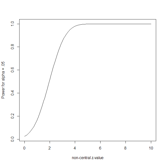
This illustrates an important asymmetry. Low or moderate observed power in a single study is highly uncertain. A point estimate of 20% or 50% power may be compatible with a wide range of true power values. But very high observed power is different. A result with z = 6 is not easily explained by a study with only 50% true power. Under 50% power, the expected z-value is near the significance threshold, not three standard errors above it. Such an extreme result could occur by chance, but it is rare.

This matters because z-values greater than 6 are not uncommon in some areas of research, especially when studies use large samples, precise measures, strong manipulations, or repeated observations. These results are not merely statistically significant. They are highly replicable under the same design and population assumptions. If a replication study fails to reproduce such a finding, the most plausible explanation is often not ordinary sampling error but some substantive difference between the original and replication studies, such as a weaker manipulation, a different population, a changed measurement procedure, or a failure to reproduce the relevant conditions.

The real difficulty concerns low power in literatures with many studies. A single borderline-significant result cannot demonstrate that a study truly had low power, because the effect-size estimate is too uncertain. But a series of significant results from studies that all appear to have low or modest power is informative in a different way. The problem is not that any one study proves low power with precision. The problem is that repeated success becomes increasingly implausible when the studies, taken together, imply low probabilities of success.

In short, post-hoc power estimates from a single study are not uniformly uninformative. They are often weak for borderline results, but they can be informative when observed evidence is very strong. High power can sometimes be demonstrated from a single study. Low power is usually harder to establish from one study and is better diagnosed from patterns across multiple studies.

Average “Post-Hoc Power” As Bias Test

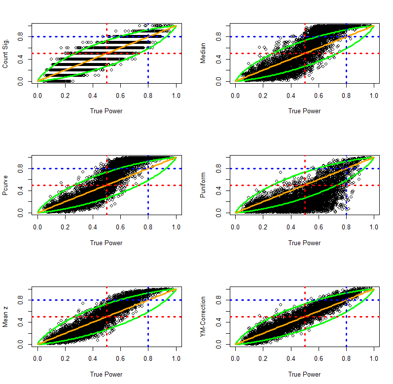
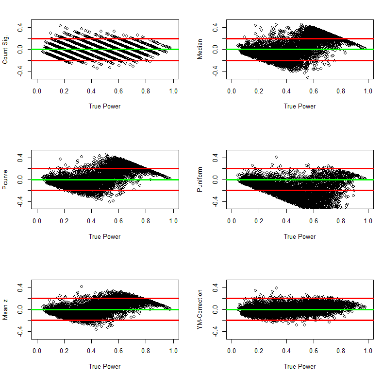
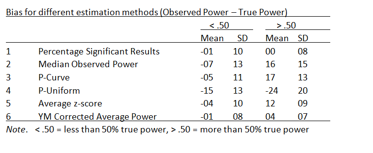
Power analyses of single studies are often uninformative because the population effect size is unknown and the observed effect-size estimate is noisy. This limitation, however, does not generalize to sets of studies. Post-hoc power analyses of multiple studies can be informative because they allow researchers to compare the expected number of significant results with the number of significant results that was actually observed. This comparison is the basis of several bias tests, including tests proposed by Ioannidis and Trikalinos (2007), Francis (2014), Schimmack (2012), and the z-curve selection model (Bartos & Schimmack, 2022; Brunner & Schimmack, 2020).

Before discussing these tests, it is important to distinguish statistical power from the unconditional probability of obtaining a significant result. In the Neyman-Pearson framework, power is the probability of rejecting a false null hypothesis. It is therefore conditional on H0 being false. After a study has been completed, however, we usually do not know whether the tested null hypothesis was true or false. A set of studies may contain some true effects and some true null hypotheses. Consequently, the expected rate of significant results in such a set is not identical to average power in the strict Neyman-Pearson sense. It is the unconditional probability that a study produces a significant result.

Bartoš and Schimmack introduced the term expected discovery rate (EDR) for this unconditional probability. The EDR is related to power, but it is also influenced by the proportion of true null hypotheses that were tested. If all tested hypotheses are false, the EDR corresponds to average power. If some tested hypotheses are true, the EDR is lower because true null hypotheses can produce significant results only as Type I errors (Sterling et al., 1995).

The EDR is useful because it can be compared with the observed discovery rate (ODR), that is, the actual proportion of significant results in a set of studies. When the ODR is much higher than the EDR, the literature contains more significant results than the population effect sizes and sample sizes of the studies could have produced. This discrepancy provides evidence of selection bias, questionable research practices, or other reporting processes that favor significant results.

This use of post-hoc power is especially important because it addresses a problem that conventional publication-bias methods often handle poorly. Funnel plots and regression-based methods can be difficult to interpret when studies are heterogeneous. A relation between sampling error and effect size may reflect publication bias, but it may also reflect real heterogeneity, differences in study design, or differences in the populations and measures used across studies. Power-based bias tests do not require effect sizes to be homogeneous in the same way. They ask a different question: given the estimated probability that each study would produce a significant result, is the observed number of significant results credible? This makes power-based bias tests a valuable complement to funnel-plot and regression-based methods.

The logic is simple. If five studies each had only a 30% probability of producing a significant result, the probability that all five would be significant is .30⁵ = .0024. A set of five significant results is therefore not impossible, but it is statistically surprising. The problem becomes even more severe in literatures with success rates above 90%, which were common in psychology before the replication crisis. In such literatures, the question is not whether a single significant result was lucky. The question is whether the entire pattern of significant results is plausible under the estimated EDR.

Publication bias also creates a problem for a priori power analyses based on completed studies. When studies are selected for significance, their effect-size estimates are inflated. Sample-size planning based on those inflated estimates will therefore overestimate the power of future replication studies. This is precisely what happened in the Reproducibility Project. The replication studies were planned to have high power based on the original published effect sizes, yet the actual success rate was much lower. This discrepancy has often been treated as puzzling, but it is exactly what should be expected when original effect sizes are inflated by selection for significance.

The more important fact is not simply that the replication success rate was 36%. A low replication rate can have many explanations. The more diagnostic fact is that the original journals had success rates above 90%, whereas the expected discovery rate was much lower. This discrepancy reveals that the published literature contained too many significant results. It also explains why the original effect-size estimates were larger than the replication effect-size estimates and why a priori power analyses based on the original studies overstated the true power of the replications.

In short, “post-hoc power” of a set of studies (i.e., the expected discovery rate) has become an important application for power analyses of completed studies. The results of this application of power analysis also have implications for a priori power analyses. A priori power analysis based on meta-analyses of previous studies with publication bias will produce inflated estimates of power and suggest sample sizes that are too small. Estimating and correction biases in these meta-analyses is therefore important to avoid high type-II error rates in replication studies.

Conclusion

After the cognitive revolution of the 1970s, the affective revolution of the 1980s, the implicit revolution of the 1990s, and the neuroscience revolution of the 2000s, psychology underwent a methodological revolution in the 2010s. This revolution revealed serious defects in how psychologists designed studies, analyzed data, and reported results. It also vindicated Cohen’s long-standing warnings about low statistical power. The replication crisis was therefore not a surprise. It was the predictable consequence of a discipline that had embraced small samples despite Cohen’s reminder that “less is more except for sample size.”

Psychological science is now more attentive to statistical power, but misconceptions about power continue to impede progress. Power analysis is increasingly accepted as a tool for planning better studies, yet researchers still disagree about how to choose the population effect size needed for a meaningful a priori power analysis. At the same time, the focus on a priori planning has encouraged the mistaken belief that power becomes irrelevant once a study has been completed. This belief has led to overly broad claims that post-hoc power calculations should not be conducted.

Giner-Sorolla et al. (2024) already recognized legitimate uses of power calculations for completed studies, especially for evaluating the sensitivity of focal tests rather than relying on sample size alone. However, they remained skeptical of observed-power calculations that use the effect-size estimate from the same completed study, because such estimates often add little beyond the p-value and remain highly uncertain.

Here, I marshal a stronger defense of power calculations based on completed studies. First, I argue that uncertainty about the population effect size is not unique to post-hoc power. Sampling error in effect-size estimates affects a priori power calculations just as much as post-hoc power calculations when both rely on empirical estimates from completed studies. Second, I argue that power calculations based on actual results are essential for evaluating the credibility of published literatures. Only the observed results of completed studies can be used to estimate the expected discovery rate and compare it with the observed discovery rate. This comparison is the basis of power-based tests of publication bias. As long as power calculations are restricted to hypothetical effect sizes, they remain planning exercises; they cannot evaluate whether a published literature contains too many significant results. In this sense, a priori power analyses have limited diagnostic consequences because they are not based on the actual pattern of published findings. By contrast, bias tests that estimate expected discovery rates can challenge the credibility of entire literatures with hundreds of statistically significant results (Chen et al., 2025).

The central problem is not whether a power calculation is conducted before or after data are collected. The central problem is uncertainty. All empirical power calculations are affected by random error, and all calculations based on published findings may be affected by systematic error, especially selection bias. A priori power analyses are not exempt from this problem. If they rely on inflated effect-size estimates from selected literatures, they will overestimate the power of future studies. Conversely, post-hoc power analyses can be informative when they are used to evaluate whether published success rates are credible given the estimated probability of significant results.

Thus, the familiar objections to “post-hoc power” identify real problems, but they misdiagnose their source. The problem is not that power is calculated after the study. The problem is that point estimates are often confused with population quantities. Terms such as “effect size” and “power” are frequently used as shorthand for noisy estimates, while the uncertainty around those estimates is ignored. Clearer language would help: researchers should distinguish effect-size estimates from population effect sizes and power estimates from actual power, and they should report point estimates together with confidence intervals whenever possible.

The future of power analysis should therefore not be limited to a priori sample-size planning. Power estimates also have an important diagnostic function. They can reveal when published literatures contain too many significant results, when effect-size estimates are likely to be inflated, and when a priori power analyses based on those estimates are misleading. Properly understood, post-hoc power analysis is not an abuse of power. It is one tool for correcting the very biases that made the replication crisis possible.

An Introduction to Z-Curve: A method for estimating mean power after selection for significance (replicability)

October 19, 2018Observed Power, Post-Hoc Power, Posteriori Power Analysis, Power, Replicability, Z-Curve, ZcurveUlrich Schimmack

UPDATE 5/13/2019 Our manuscript on the z-curve method for estimation of mean power after selection for significance has been accepted for publication in Meta-Psychology. As estimation of actual power is an important tool for meta-psychologists, we are happy that z-curve found its home in Meta-Psychology. We also enjoyed the open and constructive review process at Meta-Psychology. Definitely will try Meta-Psychology again for future work (look out for z-curve.2.0 with many new features).

Z.Curve.1.0.Meta.Psychology.In.Press

Since 2015, Jerry Brunner and I have been working on a statistical tool that can estimate mean (statitical) power for a set of studies with heterogeneous sample sizes and effect sizes (heterogeneity in non-centrality parameters and true power). This method corrects for the inflation in mean observed power that is introduced by the selection for statistical significance. Knowledge about mean power makes it possible to predict the success rate of exact replication studies. For example, if a set of studies with mean power of 60% were replicated exactly (including sample sizes), we would expect that 60% of the replication studies produce a significant result again.

Our latest manuscript is a revision of an earlier manuscript that received a revise and resubmit decision from the free, open-peer-review journal Meta-Psychology. We consider it the most authoritative introduction to z-curve that should be used to learn about z-curve, critic z-curve, or as a citation for studies that use z-curve.

Cite as “submitted for publication”.

Final.Revision.874-Manuscript in PDF-2236-1-4-20180425 mva final (002)

Feel free to ask questions, provide comments, and critic our manuscript in the comments section. We are proud to be an open science lab, and consider criticism an opportunity to improve z-curve and our understanding of power estimation.

R-CODE
Latest R-Code to run Z.Curve (Z.Curve.Public.18.10.28).
[updated 18/11/17] [35 lines of code]
call function mean.power = zcurve(pvalues,Plot=FALSE,alpha=.05,bw=.05)[1]

Z-Curve related Talks
Presentation on Z-curve and application to BS Experimental Social Psychology and (Mostly) WS-Cognitive Psychology at U Waterloo (November 2, 2018)
[Powerpoint Slides]

The Abuse of Hoenig and Heisey: A Justification of Power Calculations with Observed Effect Sizes

January 14, 2016Meta-Analysis, Observed Power, Post-Hoc Power, Posteriori Power Analysis, PowerUlrich Schimmack

In 2001, Hoenig and Heisey wrote an influential article, titled “The Abuse of Power: The Persuasive Fallacy of Power Calculations For Data Analysis.” The article has been cited over 500 times and it is commonly cited as a reference to claim that it is a fallacy to use observed effect sizes to compute statistical power.

In this post, I provide a brief summary of Hoenig and Heisey’s argument. The summary shows that Hoenig and Heisey were concerned with the practice of assessing the statistical power of a single test based on the observed effect size for this effect. I agree that it is often not informative to do so (unless the result is power = .999). However, the article is often cited to suggest that the use of observed effect sizes in power calculations is fundamentally flawed. I show that this statement is false.

The abstract of the article makes it clear that Hoenig and Heisey focused on the estimation of power for a single statistical test. “There is also a large literature advocating that power calculations be made whenever one performs a statistical test of a hypothesis and one obtains a statistically nonsignificant result” (page 1). The abstract informs readers that this practice is fundamentally flawed. “This approach, which appears in various forms, is fundamentally flawed. We document that the problem is extensive and present arguments to demonstrate the flaw in the logic” (p. 1).

Given that method articles can be difficult to read, it is possible that the misinterpretation of Hoenig and Heisey is the result of relying on the term “fundamentally flawed” in the abstract. However, some passages in the article are also ambiguous. In the Introduction Hoenig and Heisey write “we describe the flaws in trying to use power calculations for data-analytic purposes” (p. 1). It is not clear what purposes are left for power calculations if they cannot be used for data-analytic purposes. Later on, they write more forcefully “A number of authors have noted that observed power may not be especially useful, but to our knowledge a fatal logical flaw has gone largely unnoticed.” (p. 2). So readers cannot be blamed entirely if they believed that calculations of observed power are fundamentally flawed. This conclusion is often implied in Hoenig and Heisey’s writing, which is influenced by their broader dislike of hypothesis testing in general.

The main valid argument that Hoenig and Heisey make is that power analysis is based on the unknown population effect size and that effect sizes in a particular sample are contaminated with sampling error. As p-values and power estimates depend on the observed effect size, they are also influenced by random sampling error.

In a special case, when true power is 50%, the p-value matches the significance criterion. If sampling error leads to an underestimation of the true effect size, the p-value will be non-significant and the power estimate will be less than 50%. When sampling error inflates the observed effect size, p-values will be significant and power will be above 50%.

It is therefore impossible to find scenarios where observed power is high (80%) and a result is not significant, p > .05, or where observed power is low (20%) and a result is significant, p < .05. As a result, it is not possible to use observed power to decide whether a non-significant result was obtained because power was low or because power was high but the effect does not exist.

In fact, a simple mathematical formula can be used to transform p-values into observed power and vice versa (I actually got the idea of using p-values to estimate power from Hoenig and Heisey’s article). Given this perfect dependence between the two statistics, observed power cannot add additional information to the interpretation of a p-value.

This central argument is valid and it does mean that it is inappropriate to use the observed effect size of a statistical test to draw inferences about the statistical power of a significance test for the same effect (N = 1). Similarly, one would not rely on a single data point to draw inferences about the mean of a population.

However, it is common practice to aggregate original data points or to aggregated effect sizes of multiple studies to obtain more precise estimates of the mean in a population or the mean effect size, respectively. Thus, the interesting question is whether Hoenig and Heisey’s (2001) article contains any arguments that would undermine the aggregation of power estimates to obtain an estimate of the typical power for a set of studies. The answer is no. Hoenig and Heisey do not consider a meta-analysis of observed power in their discussion and their discussion of observed power does not contain arguments that would undermine the validity of a meta-analysis of post-hoc power estimates.

A meta-analysis of observed power can be extremely useful to check whether researchers’ a priori power analysis provide reasonable estimates of the actual power of their studies.

Assume that researchers in a particular field have to demonstrate that their studies have 80% power to produce significant results when an important effect is present because conducting studies with less power would be a waste of resources (although some granting agencies require power analyses, these power analyses are rarely taken seriously, so I consider this a hypothetical example).

Assume that researchers comply and submit a priori power analysis with effect sizes that are considered to be sufficiently meaningful. For example, an effect of half-a-standard deviation (Cohen’s d = .50) might look reasonable large to be meaningful. Researchers submit their grant applications with a prior power analysis that produce 80% power with an effect size of d = .50. Based on the power analysis, researchers request funding for 128 participants. A researcher plans four studies and needs $50 for each participant. The total budget is $25,600.

When the research project is completed, all four studies produced non-significant results. The observed standardized effect sizes were 0, .20, .25, and .15. Is it really impossible to estimate the realized power in these studies based on the observed effect sizes? No. It is common practice to conduct a meta-analysis of observed effect sizes to get a better estimate of the (average) population effect size. In this example, the average effect size across the four studies is d = .15. It is also possible to show that the average effect size in these four studies is significantly different from the effect size that was used for the a priori power calculation (M1 = .15, M2 = .50, Mdiff = .35, SE = 1/sqrt(512) = .044, t = .35 / .044 = 7.92, p < 1e-13). Using the more realistic effect size estimate that is based on actual empirical data rather than wishful thinking, the post-hoc power analysis yields a power estimate of 13%. The probability of obtaining non-significant results in all four studies is 57%. Thus, it is not surprising that the studies produced non-significant results. In this example, a post-hoc power analysis with observed effect sizes provides valuable information about the planning of future studies in this line of research. Either effect sizes of this magnitude are not important enough and research should be abandoned or effect sizes of this magnitude still have important practical implications and future studies should be planned on the basis of a priori power analysis with more realistic effect sizes.

Another valuable application of observed power analysis is the detection of publication bias and questionable research practices (Ioannidis and Trikalinos; 2007), Schimmack, 2012) and for estimating the replicability of statistical results published in scientific journals (Schimmack, 2015).

In conclusion, the article by Hoenig and Heisey is often used as a reference to argue that observed effect sizes should not be used for power analysis. This post clarifies that this practice is not meaningful for a single statistical test, but that it can be done for larger samples of studies.

Meta-Analysis of Observed Power: Comparison of Estimation Methods

April 1, 2015Median Observed Power, Meta-Analysis, Observed Power, Pcurve, Post-Hoc Power, Posteriori Power Analysis, Publication Bias, Puniform, Questionable Research Practices, r-index, YMCA, Yuan-Maxwell, Yuan-Maxwell Correction, Yuan-Maxwell-Corrected-AverageMeta-Analysis, Meta-Science, replicability, Replication, ScienceUlrich Schimmack

Meta-Analysis of Observed Power

Citation: Dr. R (2015). Meta-analysis of observed power. R-Index Bulletin, Vol(1), A2.

In a previous blog post, I presented an introduction to the concept of observed power. Observed power is an estimate of the true power on the basis of observed effect size, sampling error, and significance criterion of a study. Yuan and Maxwell (2005) concluded that observed power is a useless construct when it is applied to a single study, mainly because sampling error in a single study is too large to obtain useful estimates of true power. However, sampling error decreases as the number of studies increases and observed power in a set of studies can provide useful information about the true power in a set of studies.

This blog post introduces various methods that can be used to estimate power on the basis of a set of studies (meta-analysis). I then present simulation studies that compare the various estimation methods in terms of their ability to estimate true power under a variety of conditions. In this blog post, I examine only unbiased sets of studies. That is, the sample of studies in a meta-analysis is a representative sample from the population of studies with specific characteristics. The first simulation assumes that samples are drawn from a population of studies with fixed effect size and fixed sampling error. As a result, all studies have the same true power (homogeneous). The second simulation assumes that all studies have a fixed effect size, but that sampling error varies across studies. As power is a function of effect size and sampling error, this simulation models heterogeneity in true power. The next simulations assume heterogeneity in population effect sizes. One simulation uses a normal distribution of effect sizes. Importantly, a normal distribution has no influence on the mean because effect sizes are symmetrically distributed around the mean effect size. The next simulations use skewed normal distributions. This simulation provides a realistic scenario for meta-analysis of heterogeneous sets of studies such as a meta-analysis of articles in a specific journal or articles on different topics published by the same author.

Observed Power Estimation Method 1: The Percentage of Significant Results

The simplest method to determine observed power is to compute the percentage of significant results. As power is defined as the long-range percentage of significant results, the percentage of significant results in a set of studies is an unbiased estimate of the long-term percentage. The main limitation of this method is that the dichotomous measure (significant versus insignificant) is likely to be imprecise when the number of studies is small. For example, two studies can only show observed power values of 0, 25%, 50%, or 100%, even if true power were 75%. However, the percentage of significant results plays an important role in bias tests that examine whether a set of studies is representative. When researchers hide non-significant results or use questionable research methods to produce significant results, the percentage of significant results will be higher than the percentage of significant results that could have been obtained on the basis of the actual power to produce significant results.

Observed Power Estimation Method 2: The Median

Schimmack (2012) proposed to average observed power of individual studies to estimate observed power. Yuan and Maxwell (2005) demonstrated that the average of observed power is a biased estimator of true power. It overestimates power when power is less than 50% and it underestimates true power when power is above 50%. Although the bias is not large (no more than 10 percentage points), Yuan and Maxwell (2005) proposed a method that produces an unbiased estimate of power in a meta-analysis of studies with the same true power (exact replication studies). Unlike the average that is sensitive to skewed distributions, the median provides an unbiased estimate of true power because sampling error is equally likely (50:50 probability) to inflate or deflate the observed power estimate. To avoid the bias of averaging observed power, Schimmack (2014) used median observed power to estimate the replicability of a set of studies.

Observed Power Estimation Method 3: P-Curve’s KS Test

Another method is implemented in Simonsohn’s (2014) pcurve. Pcurve was developed to obtain an unbiased estimate of a population effect size from a biased sample of studies. To achieve this goal, it is necessary to determine the power of studies because bias is a function of power. The pcurve estimation uses an iterative approach that tries out different values of true power. For each potential value of true power, it computes the location (quantile) of observed test statistics relative to a potential non-centrality parameter. The best fitting non-centrality parameter is located in the middle of the observed test statistics. Once a non-central distribution has been found, it is possible to assign each observed test-value a cumulative percentile of the non-central distribution. For the actual non-centrality parameter, these percentiles have a uniform distribution. To find the best fitting non-centrality parameter from a set of possible parameters, pcurve tests whether the distribution of observed percentiles follows a uniform distribution using the Kolmogorov-Smirnov test. The non-centrality parameter with the smallest test statistics is then used to estimate true power.

Observed Power Estimation Method 4: P-Uniform

van Assen, van Aert, and Wicherts (2014) developed another method to estimate observed power. Their method is based on the use of the gamma distribution. Like the pcurve method, this method relies on the fact that observed test-statistics should follow a uniform distribution when a potential non-centrality parameter matches the true non-centrality parameter. P-uniform transforms the probabilities given a potential non-centrality parameter with a negative log-function (-log[x]). These values are summed. When probabilities form a uniform distribution, the sum of the log-transformed probabilities matches the number of studies. Thus, the value with the smallest absolute discrepancy between the sum of negative log-transformed percentages and the number of studies provides the estimate of observed power.

Observed Power Estimation Method 5: Averaging Standard Normal Non-Centrality Parameter

In addition to these existing methods, I introduce to novel estimation methods. The first new method converts observed test statistics into one-sided p-values. These p-values are then transformed into z-scores. This approach has a long tradition in meta-analysis that was developed by Stouffer et al. (1949). It was popularized by Rosenthal during the early days of meta-analysis (Rosenthal, 1979). Transformation of probabilities into z-scores makes it easy to aggregate probabilities because z-scores follow a symmetrical distribution. The average of these z-scores can be used as an estimate of the actual non-centrality parameter. The average z-score can then be used to estimate true power. This approach avoids the problem of averaging power estimates that power has a skewed distribution. Thus, it should provide an unbiased estimate of true power when power is homogenous across studies.

Observed Power Estimation Method 6: Yuan-Maxwell Correction of Average Observed Power

Yuan and Maxwell (2005) demonstrated a simple average of observed power is systematically biased. However, a simple average avoids the problems of transforming the data and can produce tighter estimates than the median method. Therefore I explored whether it is possible to apply a correction to the simple average. The correction is based on Yuan and Maxwell’s (2005) mathematically derived formula for systematic bias. After averaging observed power, Yuan and Maxwell’s formula for bias is used to correct the estimate for systematic bias. The only problem with this approach is that bias is a function of true power. However, as observed power becomes an increasingly good estimator of true power in the long run, the bias correction will also become increasingly better at correcting the right amount of bias.

The Yuan-Maxwell correction approach is particularly promising for meta-analysis of heterogeneous sets of studies such as sets of diverse studies in a journal. The main advantage of this method is that averaging of power makes no assumptions about the distribution of power across different studies (Schimmack, 2012). The main limitation of averaging power was the systematic bias, but Yuan and Maxwell’s formula makes it possible to reduce this systematic bias, while maintaining the advantage of having a method that can be applied to heterogeneous sets of studies.

RESULTS

Homogeneous Effect Sizes and Sample Sizes

The first simulation used 100 effect sizes ranging from .01 to 1.00 and 50 sample sizes ranging from 11 to 60 participants per condition (Ns = 22 to 120), yielding 5000 different populations of studies. The true power of these studies was determined on the basis of the effect size, sample size, and the criterion p < .025 (one-tailed), which is equivalent to .05 (two-tailed). Sample sizes were chosen so that average power across the 5,000 studies was 50%. The simulation drew 10 random samples from each of the 5,000 populations of studies. Each sample of a study simulated a between-subject design with the given population effect size and sample size. The results were stored as one-tailed p-values. For the meta-analysis p-values were converted into z-scores. To avoid biases due to extreme outliers, z-scores greater than 5 were set to 5 (observed power = .999).

The six estimation methods were then used to compute observed power on the basis of samples of 10 studies. The following figures show observed power as a function of true power. The green lines show the 95% confidence interval for different levels of true power. The figure also includes red dashed lines for a value of 50% power. Studies with more than 50% observed power would be significant. Studies with less than 50% observed power would be non-significant. The figures also include a blue line for 80% true power. Cohen (1988) recommended that researchers should aim for a minimum of 80% power. It is instructive how accurate estimation methods are in evaluating whether a set of studies met this criterion.

The histogram shows the distribution of true power across the 5,000 populations of studies.

The histogram shows that the simulation covers the full range of power. It also shows that high-powered studies are overrepresented because moderate to large effect sizes can achieve high power for a wide range of sample sizes. The distribution is not important for the evaluation of different estimation methods and benefits all estimation methods equally because observed power is a good estimator of true power when true power is close to the maximum (Yuan & Maxwell, 2005).

The next figure shows scatterplots of observed power as a function of true power. Values above the diagonal indicate that observed power overestimates true power. Values below the diagonal show that observed power underestimates true power.

Visual inspection of the plots suggests that all methods provide unbiased estimates of true power. Another observation is that the count of significant results provides the least accurate estimates of true power. The reason is simply that aggregation of dichotomous variables requires a large number of observations to approximate true power. The third observation is that visual inspection provides little information about the relative accuracy of the other methods. Finally, the plots show how accurate observed power estimates are in meta-analysis of 10 studies. When true power is 50%, estimates very rarely exceed 80%. Similarly, when true power is above 80%, observed power is never below 50%. Thus, observed power can be used to examine whether a set of studies met Cohen’s recommended guidelines to conduct studies with a minimum of 80% power. If observed power is 50%, it is nearly certain that the studies did not have the recommended 80% power.

To examine the relative accuracy of different estimation methods quantitatively, I computed bias scores (observed power – true power). As bias can overestimate and underestimate true power, the standard deviation of these bias scores can be used to quantify the precision of various estimation methods. In addition, I present the mean to examine whether a method has large sample accuracy (i.e. the bias approaches zero as the number of simulations increases). I also present the percentage of studies with no more than 20% points bias. Although 20% bias may seem large, it is not important to estimate power with very high precision. When observed power is below 50%, it suggests that a set of studies was underpowered even if the observed power estimate is an underestimation.

The quantitative analysis also shows no meaningful differences among the estimation methods. The more interesting question is how these methods perform under more challenging conditions when the set of studies are no longer exact replication studies with fixed power.

Homogeneous Effect Size, Heterogeneous Sample Sizes

The next simulation simulated variation in sample sizes. For each population of studies, sample sizes were varied by multiplying a particular sample size by factors of 1 to 5.5 (1.0, 1.5,2.0…,5.5). Thus, a base-sample-size of 40 created a range of sample sizes from 40 to 220. A base-sample size of 100 created a range of sample sizes from 100 to 2,200. As variation in sample sizes increases the average sample size, the range of effect sizes was limited to a range from .004 to .4 and effect sizes were increased in steps of d = .004. The histogram shows the distribution of power in the 5,000 population of studies.

The simulation covers the full range of true power, although studies with low and very high power are overrepresented.

The results are visually not distinguishable from those in the previous simulation.

The quantitative comparison of the estimation methods also shows very similar results.

In sum, all methods perform well even when true power varies as a function of variation in sample sizes. This conclusion may not generalize to more extreme simulations of variation in sample sizes, but more extreme variations in sample sizes would further increase the average power of a set of studies because the average sample size would increase as well. Thus, variation in effect sizes poses a more realistic challenge for the different estimation methods.

Heterogeneous, Normally Distributed Effect Sizes

The next simulation used a random normal distribution of true effect sizes. Effect sizes were simulated to have a reasonable but large variation. Starting effect sizes ranged from .208 to 1.000 and increased in increments of .008. Sample sizes ranged from 10 to 60 and increased in increments of 2 to create 5,000 populations of studies. For each population of studies, effect sizes were sampled randomly from a normal distribution with a standard deviation of SD = .2. Extreme effect sizes below d = -.05 were set to -.05 and extreme effect sizes above d = 1.20 were set to 1.20. The first histogram of effect sizes shows the 50,000 population effect sizes. The histogram on the right shows the distribution of true power for the 5,000 sets of 10 studies.

The plots of observed and true power show that the estimation methods continue to perform rather well even when population effect sizes are heterogeneous and normally distributed.

The quantitative comparison suggests that puniform has some problems with heterogeneity. More detailed studies are needed to examine whether this is a persistent problem for puniform, but given the good performance of the other methods it seems easier to use these methods.

Heterogeneous, Skewed Normal Effect Sizes

The next simulation puts the estimation methods to a stronger challenge by introducing skewed distributions of population effect sizes. For example, a set of studies may contain mostly small to moderate effect sizes, but a few studies examined large effect sizes. To simulated skewed effect size distributions, I used the rsnorm function of the fGarch package. The function creates a random distribution with a specified mean, standard deviation, and skew. I set the mean to d = .2, the standard deviation to SD = .2, and skew to 2. The histograms show the distribution of effect sizes and the distribution of true power for the 5,000 sets of studies (k = 10).

This time the results show differences between estimation methods in the ability of various estimation methods to deal with skewed heterogeneity. The percentage of significant results is unbiased, but is imprecise due to the problem of averaging dichotomous variables. The other methods show systematic deviations from the 95% confidence interval around the true parameter. Visual inspection suggests that the Yuan-Maxwell correction method has the best fit.

This impression is confirmed in quantitative analyses of bias. The quantitative comparison confirms major problems with the puniform estimation method. It also shows that the median, p-curve, and the average z-score method have the same slight positive bias. Only the Yuan-Maxwell corrected average power shows little systematic bias.

To examine biases in more detail, the following graphs plot bias as a function of true power. These plots can reveal that a method may have little average bias, but has different types of bias for different levels of power. The results show little evidence of systematic bias for the Yuan-Maxwell corrected average of power.

The following analyses examined bias separately for simulation with less or more than 50% true power. The results confirm that all methods except the Yuan-Maxwell correction underestimate power when true power is below 50%. In contrast, most estimation methods overestimate true power when true power is above 50%. The exception is puniform which still underestimated true power. More research needs to be done to understand the strange performance of puniform in this simulation. However, even if p-uniform could perform better, it is likely to be biased with skewed distributions of effect sizes because it assumes a fixed population effect size.

Conclusion

This investigation introduced and compared different methods to estimate true power for a set of studies. All estimation methods performed well when a set of studies had the same true power (exact replication studies), when effect sizes were homogenous and sample sizes varied, and when effect sizes were normally distributed and sample sizes were fixed. However, most estimation methods were systematically biased when the distribution of effect sizes was skewed. In this situation, most methods run into problems because the percentage of significant results is a function of the power of individual studies rather than the average power.

The results of these analyses suggest that the R-Index (Schimmack, 2014) can be improved by simply averaging power and then applying the Yuan-Maxwell correction. However, it is important to realize that the median method tends to overestimate power when power is greater than 50%. This makes it even more difficult for the R-Index to produce an estimate of low power when power is actually high. The next step in the investigation of observed power is to examine how different methods perform in unrepresentative (biased) sets of studies. In this case, the percentage of significant results is highly misleading. For example, Sterling et al. (1995) found percentages of 95% power, which would suggest that studies had 95% power. However, publication bias and questionable research practices create a bias in the sample of studies that are being published in journals. The question is whether other observed power estimates can reveal bias and can produce accurate estimates of the true power in a set of studies.

Replicability-Index

Improving the replicability of empirical research