In a blog post on Andrew Gelman’s blog, Erik van Zwet voiced serious concerns about the performance of z-curve, a meta-analytic method to detect selection bias. The main concern was that z-curve failed to detect selection bias in a scenario where most observed data come from high-powered studies (noncentrality parameter z = 4) but some come from tests of true H0 (effect size is zero, z = 0). In some cases, there may only be a couple of false positive results and that provides too little information about the file drawer of missing tests of H0).
The first problem that I already addressed is that EvZ’s criticism was invalid because it generalized from a single unrealistic scenario to all other situations and did not mention that z-curve had been validated and performed well in these situations (Schimmack, 2026).
Another selection bias in EvZ’s criticism of z-curve is that he only examined the performance of z-curve and did not compare it to the performance of other models. One advantage of z-curve is that it works even if there is little or no variation in sample sizes, which is a requirement for all regression based methods like Funnel plots, Eggert regression, or PET/PEESE. Thus, the most relevant competitor for z-curve are selection models like Vevea and Wood’s (2005) random-effects, step-function model implemented in the r-package weightr.
I tested the model using the same simulation design that was used to examine the performance of z-curve with identical data. Here I focus on the EvZ scenario where most statistically significant results come tests with high power (d = .6, N = 200, z ~ 4.24, power ~ 98%). Thus, there are few non-significant results that can be suppressed by publication bias.
All simulations had 70% selection bias. That is only 30% of the non-significant results were reported and the distribution was flat. First I examined the performance of weightr with k = 100 significant results. All 100 simulations failed to provide estimates of the selection weight for non-significant results. With k = 300 significant results, bias was detected 92% of the time. With k = 1,000, bias was detected in all 100 simulations.
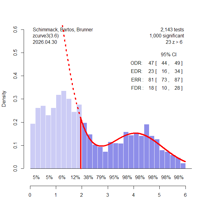
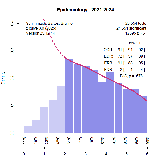
I then examined performance when 20% of the significant results are false positives – and the other 80% come from the same high-powered distribution as before. Figure 1 shows results for a run with k = 1,000 significant results for z-curve. With k = 1,000 z-curve has no problem detecting the selection bias because the distribution of the significant results is clearly bimodal with the mode for the studies with weak power in the non-significant range. Z-curve shows that there are more observed significant results, observed discover rate ODR = 47% than z-curve predicts based on the distribution of the significant results, expected discovery rate, EDR = 23%. The difference is highly significant, p < .000001.
In contrast, the step-function model falsely interprets the higher percentage of non-significant results as evidence that significant results are missing, w(p-value in .025 to .5 range) = 2.24, 95% 2.05 to 2.43. The reason is that the model does not allow for bimodal distributions and assumes a normal distribution of effect sizes, which also implies a normal distribution of z-values when sample sizes are fixed. This problem with the step-function selection model was already reported by Hedges & Vevea (1995). When the simulated data matched the assumed normal distribution, the model worked well. When the distribution did not match the assumed distribution, the model produced bias estimates. The advantage of z-curve is that it does not make a strong distribution assumption and allows for bimodal distributions like the one in Figure 1.
Conclusion
This blog post shows further evidence that EvZ’ expression of concerns about z-curve are biased and do not provide a balanced account of the strengths and weaknesses of z-curve. It is unreasonable to expect a model to perform well in an edge case that also provides problems for other models. In fact, z-curve handles the problem of bimodal distributions better than other models that assume unimodal distributions. If a heterogeneous literature contains a mixture of studies that tested true and false hypotheses, z-curve is actually the superior method and there are no alternatives because most meta-analytic methods were designed to analyze data where all studies are fairly similar and variation in population effect sizes is small. However, many meta-analyses in psychology show evidence of large heterogeneity and the true distribution of effect sizes across studies is unknown. For these kind of data, z-curve is currently the most appropriate statistical tool.
The caliper test is a statistical method for detecting publication bias introduced by Gerber and Malhotra (2008a, 2008b). It tests whether the distribution of test statistics is continuous and approximately locally symmetric around a significance threshold, typically z = 1.96, corresponding to p = .05. The key assumption is that, in the absence of publication bias or p-hacking, the expected density of z-scores in a narrow band just above the threshold should be approximately equal to the expected density just below it. A significant excess of results just above the threshold suggests that researchers or publication processes have shifted results across the boundary, either through selective reporting or analytical flexibility.
Procedure
Published p-values are converted to z-scores (z = Φ⁻¹(1 − p/2)). A caliper of width w is placed symmetrically around the threshold, creating two bins: one from 1.96 to 1.96 + w (just significant) and one from 1.96 − w to 1.96 (just nonsignificant). Under the null hypothesis of no bias, the counts in the two bins should be equal. The test is conducted as a one-sided binomial test with expected probability 0.50. Gerber and Malhotra (2008a) recommended bandwidths of 5%, 10%, 15%, and 20% of the threshold value. A 10% caliper around z = 1.96, for example, compares counts in the intervals [1.764, 1.96) and [1.96, 2.156].
Applications
Gerber and Malhotra applied the caliper test to leading political science journals (APSR, AJPS) and sociology journals (ASR, AJS) and found strong evidence of publication bias (Gerber & Malhotra, 2008a; Gerber & Malhotra, 2008b). The test was subsequently adopted in economics, most notably by Brodeur, Lé, Sangnier, and Zylberberg (2016) and Brodeur, Cook, and Heyes (2020), who documented significant bunching of test statistics just above conventional thresholds across top economics journals. Berning and Weiß (2016) applied the caliper test to German social science journals, again finding evidence of bias. The test has become a standard tool in the meta-science toolkit for discipline-wide assessments of publication practices.
Strengths
The caliper test has several practical advantages. The logic is intuitive and easy to communicate. It requires only test statistics or p-values, not standardized effect sizes, making it applicable to heterogeneous literatures where effect-size metrics vary across studies and designs. For discipline-wide analyses where studies address different research questions with different effects, the caliper test avoids the strong assumptions about comparability or homogeneity required by many other methods.
Limitations
The caliper test’s local-symmetry assumption is exact for normally distributed z-values only when the noncentrality parameter equals the critical value. For the conventional threshold z = 1.96, this corresponds to a study with approximately 50% power. If power is lower, the expected distribution slopes downward across the threshold, producing more just-nonsignificant than just-significant results. If power is higher, the distribution slopes upward across the threshold, producing more just-significant than just-nonsignificant results even in the absence of publication bias. Thus, deviations from caliper symmetry can reflect the power distribution of studies rather than selective publication or p-hacking.
This vulnerability becomes more influential with wider caliper intervals. With negative slopes near the threshold, as in low-powered settings, the assumption of local flatness reduces the power of the caliper test to detect publication bias. With positive slopes near the threshold, as in high-powered settings, there are more observations in the interval above the criterion value than below it even without bias. Thus, the caliper test can falsely identify publication bias when the literature has high power or when the mixture distribution slopes upward around the significance threshold. It is therefore unclear whether positive caliper-test results in some applications reflect bias or the expected shape of the z-value distribution.
Schneck (2017) conducted a Monte Carlo simulation comparing the caliper test to Egger’s test, p-uniform, and the test for excess significance (TES). He found that the 5% caliper maintained acceptable false-positive rates but had low power with fewer than 1,000 studies. The 10% and 15% calipers showed inflated false-positive rates at large K, because wider calipers span a larger portion of the density curve where the local-uniformity assumption can break down. Schneck recommended the 5% caliper for discipline-wide analyses with large K. However, a small caliper does not solve the problem of true asymmetric distributions. With large K, even small departures from local symmetry can be estimated precisely, and the caliper test can become significant even if there is no publication bias.
Simulation studies using z-curve’s heterogeneous effect-size framework reveal the problem more starkly. In a simulation with high average power, fewer than 200 studies, and no bias, the caliper test detected bias 100% of the time. Thus, the test should not be interpreted as evidence of publication bias without inspecting the expected or observed shape of the z-value distribution.
This is not merely a calibration problem that can be fixed by adjusting the significance level or caliper width. Narrower calipers can reduce curvature-induced artifacts, but they cannot remove the conceptual mismatch between what the test assumes, local symmetry, and the actual distribution of z-values when the density slopes across the threshold.
This limitation is not shared by all bias-detection methods. Methods that model the full distribution of z-scores, such as z-curve (Brunner & Schimmack, 2020; Bartoš & Schimmack, 2022), can estimate the expected shape of the z-value distribution under heterogeneous power and selection. The advantage of the caliper test is that it can have high power to detect threshold-related discontinuities in some conditions. Its disadvantage is that it can also provide false evidence of bias when the expected distribution is asymmetric. Therefore, the caliper test should be used together with a plot of the z-value distribution. A positive slope for significant values is a red flag because it violates the local-symmetry assumption of the caliper test.
Summary
The caliper test is a simple, widely used tool for detecting threshold-related publication bias in large literatures. It is most reliable when the expected distribution of test statistics is approximately locally symmetric around the significance threshold in the absence of bias. In literatures where the z-value distribution slopes across the threshold — whether because of high power, low power, or heterogeneous true effects — the test can mistake the expected shape of the distribution for evidence of selective publication or p-hacking. This problem is especially relevant in discipline-wide analyses in the social sciences, where studies often address different hypotheses, use different designs, and have heterogeneous statistical power. Researchers using the caliper test in such settings should interpret positive results with caution and consider model-based alternatives that account for the expected shape of the z-score distribution.
References
Bartoš, F., & Schimmack, U. (2022). Z-curve 2.0: Estimating replication rates and discovery rates. Meta-Psychology, 6, MP.2020.2720.
Berning, C. C., & Weiß, B. (2016). Publication bias in the German social sciences: An application of the caliper test to three top-tier German social science journals. Quality & Quantity, 50, 901–917.
Brodeur, A., Cook, N., & Heyes, A. (2020). Methods matter: p-hacking and publication bias in causal analysis in economics. American Economic Review, 110(11), 3634–3660.
Brodeur, A., Lé, M., Sangnier, M., & Zylberberg, Y. (2016). Star Wars: The empirics strike back. American Economic Journal: Applied Economics, 8(1), 1–32.
Brunner, J., & Schimmack, U. (2020). Estimating population mean power under conditions of heterogeneity and selection for significance. Meta-Psychology, 4, MP.2018.874.
Gerber, A. S., & Malhotra, N. (2008a). Do statistical reporting standards affect what is published? Publication bias in two leading political science journals. Quarterly Journal of Political Science, 3(3), 313–326.
Gerber, A. S., & Malhotra, N. (2008b). Publication bias in empirical sociological research: Do arbitrary significance levels distort published results? Sociological Methods & Research, 37(1), 3–30.
Gerber, A. S., Malhotra, N., Dowling, C. M., & Doherty, D. (2010). Publication bias in two political behavior literatures. American Politics Research, 38(4), 591–613.
Schneck, A. (2017). Examining publication bias — a simulation-based evaluation of statistical tests on publication bias. PeerJ, 5, e4115.
Concerns about research credibility have stimulated the growth of meta-science, a field that examines the reproducibility, robustness, and replicability of scientific findings (Ioannidis, 2005; Munafò et al., 2017). This literature has documented publication bias, low statistical power, inflated effect size estimates, and disappointing replication rates in some areas of research (Button et al., 2013; Ioannidis, 2005; Open Science Collaboration, 2015; Tyner et al., 2026). While initial studies focused on psychology and neuroscience, but a recent article suggested that the problems are more general. Tyner et al. (2026) reported that only about 50% of originally significant claims were successfully replicated.
A replication rate of 50% invites different interpretations. An optimistic interpretation is that most original studies detected effects in the correct direction, but that the average probability of obtaining another significant result in a new sample was only about 50%. In this scenario, selective publication of significant results inflates observed effect sizes, so replication studies often fail even when the original studies were not false positives. Many of the failures are therefore false negatives. A pessimistic interpretation is that many original results were false positives, whereas the remaining studies examined true effects with high power. In that case, the same 50% replication rate could arise from a mixture of null effects and highly powered true effects. Thus, the average replication rate alone is consistent with very different underlying realities.
To move beyond average replication rates, it is necessary to avoid reducing results to a dichotomy of significant versus non-significant. A cutoff at z = 1.96 is useful for decision making, but it discards quantitative information about the strength of evidence. A result with z = 6 provides much stronger evidence for a positive effect than a result with z = 2, just as z = -6 provides much stronger evidence for a negative effect than z = -2. This point is straightforward, but broad evaluations of replication outcomes have largely ignored differences in original evidential strength.
I used z-curve to examine heterogeneity in the strength of evidence across the original significant findings included in the two large replication projects (Brunner & Schimmack, 2020; Bartoš & Schimmack, 2022). Z-curve uses the distribution of significant z-values and corrects for the inflation in observed test statistics introduced by selection for significance. It provides two key estimates. The first is the Expected Replication Rate (ERR), which is the average probability that a significant result would be significant again in an exact replication with a new sample of the same size. The second is the Expected Discovery Rate (EDR), which is the estimated proportion of all studies, including unpublished non-significant ones, that would be expected to yield a significant result.
The EDR can be used to evaluate publication bias and to derive an upper bound on the false discovery rate using Sorić’s (1989) formula. Performance of z-curve has been examined in extensive simulation studies, which show that its 95% confidence intervals perform well when at least 100 significant results are available (Bartoš & Schimmack, 2022). Because z-curve is designed to accommodate heterogeneity in evidential strength, it is especially suitable for a diverse set of studies such as those included in the replication projects. Previous applications have shown substantial variation in ERR and EDR across research areas (Schimmack, 2020; Schimmack & Bartoš, 2023; Soto & Schimmack, 2024; Credé & Sotola, 2024; Sotola, 2022, 2024).”One limitation of previous applications is that they sometimes relied on automatically extracted p-values or focused on specific literatures. The replication projects provide gold-standard test statistics from a representative sample of social science research, avoiding both concerns. This makes it possible to examine heterogeneity in replicability across a broad range of research areas.
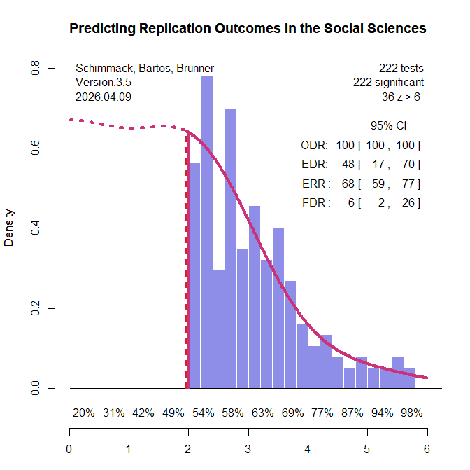
All original studies in the two replication projects were eligible for inclusion. For articles with multiple claims, the focal claim was identified from the abstract using a large language model (see OSF for details and cross-validation). When exact p-values were not reported in the project materials, the original articles were consulted to recover the necessary information. Articles without exact p-values were excluded. Original studies that claimed an effect without meeting the conventional significance threshold of p < .05 were also excluded. A small number of studies were further excluded because the replication reports did not provide sufficient information to evaluate the replication outcome. This screening process yielded k = 222 significant results (k1 = 88, k2 = 134), including k = 130 from psychology and k = 92 from other social sciences. The replication rate in this subset was similar to that in the full set of studies: 43% overall (project 1: 33%, project 2: 49%; psychology: 37%; other social sciences: 51%; see OSF for details). Figure 1 shows the z-curve analysis of these 222 original significant results.
The most striking result is that the expected replication rate (ERR) is substantially higher than the observed replication rate in the replication studies (68% versus 42%). Even the lower bound of the 95% confidence interval for the ERR, 59%, exceeds the observed replication rate. This discrepancy is especially noteworthy because the replication studies often used larger sample sizes than the original studies, which should have increased, not decreased, the probability of obtaining a significant result. Thus, the lower effect sizes observed in the replication studies cannot be attributed to regression to the mean alone. An additional factor appears to be that population effect sizes in the replication studies were systematically smaller than in the original studies.
Z-curve also limits the range of scenarios that are compatible with the data. The estimated EDR of 48% implies that no more than 6% of the significant results can be false positive results (Soric, 1989). Even the lower limit of the EDR confidence interval, 17%, limits the false positive rate to no more than 26%. With 50% replication failures, this suggests that no more than half of the replication failures are false positives. This finding shows the importance of distinguishing clearly between replication rates and false positive rates (Maxwell et al., 2015).
The false positive risk also varies as a function of the significance criterion. Marginally significant results are more likely to be false positives than results with high z-values (Benjamin et al., 2018). Z-curve makes it possible to address Benjamini and Hechtlinger’s (2014) call to control, rather than merely estimate, the science-wise false discovery rate. A stricter alpha criterion reduces the discovery rate, but it reduces the false discovery rate more. Benjamin et al. (2018) suggested reducing the false positive risk by lowering the significance criterion to alpha = .005. A z-curve analysis with this criterion estimated the FDR at 2% and the upper limit of the 95% CI was 6%. This finding provides empirical support for Benjamin et al.’s (2018) suggestion. It also addresses Lakens et al.’s (2018) concern that alpha levels should be justified. Here the strength of evidence provides the justification. In other literatures, alpha = .01 is sufficient to keep the FDR below 5% (Schimmack & Bartoš, 2023; Soto & Schimmack, 2024), but sometimes even alpha = .001 is insufficient to control false positives (Chen et al., 2025; Schimmack, 2025).
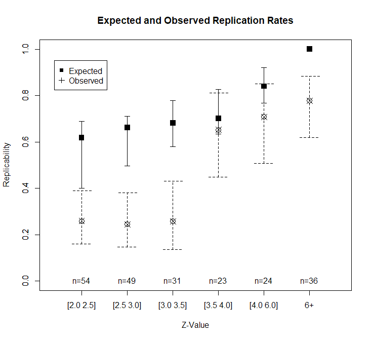
Heterogeneity in strength of evidence also makes it possible to predict replication outcomes as a function of z-values. Figure 1 shows power for z-value intervals below the x-axis. Expected replication rates increase from 54% for just significant results to over 90% for z-values greater than 5. Another 36 z-values have z-values greater than 6 that are practically guaranteed to replicate in exact replication studies. Figure 2 shows the expected replication rates and the observed replication rates for z-value ranges.
Studies with modest evidence (z = 2 to 3.5) replicate at significantly lower rates than expected based on z-curve. As expected, replication rates increase with stronger evidence. Given the small number of observations per bin, it is not possible to test whether z-curve predictions remain too optimistic at moderate z-values. The most surprising finding is that observed replication rates for studies with strong evidence (z > 6) fall below the expected rate.
In exploratory analyses, I examined possible reasons for these surprising replication failures. I used two large language models (ChatGPT and Claude) to score the replication reports of studies with strong original evidence (z > 6). Studies were coded on five dimensions (match of populations, materials, design, time period, and implementation) with scores from 0 to 2 each to produce total scores ranging from 0 to 10. Inter-rater agreement for the total scores was high, ICC(A,1) = .85, 95%CI = .73, .92. I averaged the two scores and used a total of 7 or higher as the criterion for a close match. Of the 24 close replications, 21 were successful (88%). Of the 12 studies that were not close replications, only 6 were successful (50%).
I further examined the three close replications that failed. While Farris et al. (2008) closely matched the original in many aspects, the original participants were from the US and the replication was conducted in the UK. Subsequent studies have replicated the finding with US samples (Farris et al., 2009/2010; Treat et al., 2017), ruling out a simple false positive explanation. The replication failure of Hurst and Kavanagh (2017) likely reflects a sampling problem in the original study. Participants from the general population and users of community mental health services were analyzed in a single analysis, which can inflate effect sizes (Preacher et al., 2005). McDevitt examined the influence of plumbing business names starting with numbers or A to be first in the yellow pages. A replication in 2020 cannot reproduce this effect because google searches replaced yellow pages.
While these exploratory results are based on a small sample, they support the broader claim that original results with strong evidence (z > 6) are likely to replicate in close replications and that failures may stem from meaningful differences in study design.
Conclusion
Z-curve analysis of two major replication projects reveals that replicability in the social sciences is not a single number. The expected replication rate based on the strength of original evidence (68%) substantially exceeds the observed replication rate (42%), indicating that effect size shrinkage beyond statistical regression to the mean contributes to replication failures. The false discovery rate is low (6%), confirming that most replication failures reflect reduced effect sizes rather than false positives. Adjusting the significance criterion to alpha = .005 reduces the estimated false discovery rate to 2%.
The most practically useful finding is that original results with strong evidence (z > 6) are highly replicable when the replication closely matches the original study design (88% success rate). Replication failures among these strong results were attributable to identifiable differences between the original and replication studies — different populations, changed market conditions, or heterogeneous samples. This suggests that the strength of statistical evidence, combined with methodological similarity, is a reliable predictor of replication success.
These findings argue against treating all significant results as equally credible and against interpreting average replication rates as informative about any particular study. Replicability is predictable from information already available in the original publication.
In the interest of open science, this blog post summarizes a private email exchange between Uri Simonsohn — principal developer of p-curve — and me — principal developer of z-curve. The correspondence itself is not reproduced here at Simonsohn’s request. I used AI throughout the communication, and this account of the exchange was written by Claude, who was asked to write it from a neutral third-party perspective. This does not rule out the possibility of bias, but Uri is welcome to use the comment section to share his own perspective — an option that is not available on his own blog, DataColada.
Key Points
I shared simulations showing that p-curve overestimates average power under realistic heterogeneity while z-curve does not. Simonsohn did not challenge these results.
Simonsohn’s own public position since 2018 is that p-curve is biased when some studies have power above 90%. Uncertainty about effect sizes guarantees that real data will include such studies, making bias the norm rather than the exception.
Simonsohn argued that average power is not a meaningful quantity under heterogeneity. If so, the p-curve app should stop displaying it. If average power is meaningful, z-curve estimates it better.
P-curve confidence intervals do not have 95% coverage. Z-curve.3.0 has 95% coverage even with homogeneous data.
Z-curve provides information that p-curve cannot: estimates of average power for all studies (EDR), quantification of publication bias, and bounds on the false discovery risk.
Simonsohn did not address any of these points. His public position remains unchanged from 2018.
I shared simulations showing that p-curve overestimates average power under realistic heterogeneity while z-curve does not. Simonsohn did not challenge these results. Simonsohn’s own public position since 2018 is that p-curve is biased when some studies have power above 90%. Uncertainty about effect sizes guarantees that real data will include such studies, making bias the norm rather than the exception. Simonsohn argued that average power is not a meaningful quantity under heterogeneity. If so, the p-curve app should stop displaying it. If average power is meaningful, z-curve estimates it better. P-curve does not provide confidence intervals for its power estimates. Z-curve does, with 95% coverage validated across a wide range of simulation conditions. Z-curve provides information that p-curve cannot: estimates of average power for all studies (EDR), quantification of publication bias, and bounds on the false discovery risk. Simonsohn did not address any of these points. His public position remains unchanged from 2018.
I shared simulations showing that p-curve overestimates average power under realistic heterogeneity while z-curve does not. Simonsohn did not challenge these results. Simonsohn’s own public position since 2018 is that p-curve is biased when some studies have power above 90%. Uncertainty about effect sizes guarantees that real data will include such studies, making bias the norm rather than the exception. Simonsohn argued that average power is not a meaningful quantity under heterogeneity. If so, the p-curve app should stop displaying it. If average power is meaningful, z-curve estimates it better. P-curve does not provide confidence intervals for its power estimates. Z-curve does, with 95% coverage validated across a wide range of simulation conditions. Z-curve provides information that p-curve cannot: estimates of average power for all studies (EDR), quantification of publication bias, and bounds on the false discovery risk. Simonsohn did not address any of these points. His public position remains unchanged from 2018.
Selection Models: P-Curve and Z-Curve
P-curve and z-curve are both methods that use the distribution of significant p-values to estimate the average statistical power of a set of studies. They share the same goal but differ in a critical respect: p-curve fits a single power parameter to the data, assuming all studies have the same power, while z-curve fits a mixture model that allows power to vary across studies. When power is truly homogeneous, p-curve’s simpler model is more efficient. When power is heterogeneous — as it typically is in meta-analyses of conceptual replications — p-curve produces inflated estimates with confidence intervals that are too narrow (Brunner & Schimmack, 2020). The question at the center of this exchange was whether, and under what conditions, this difference matters in practice.
The Opening: Procedural Deflection
The exchange began when Schimmack presented evidence that p-curve overestimated average power in the Reproducibility Project data. Simonsohn’s initial response did not address the overestimation. Instead, he objected that the data had not been presented in the format of a p-curve disclosure table — a procedural requirement he had developed for auditing p-curve analyses. Schimmack pointed out that the Reproducibility Project had a uniquely transparent selection process, with key findings identified collaboratively and often with input from original authors, making the disclosure table requirement a matter of form rather than substance. Simonsohn did not contest this point but instead pivoted to personal history, characterizing the dispute as a grudge, and closed the conversation with “I will switch gears and return to my current interests.”
The Simulations: A Deck Stacked for P-Curve
Several weeks later, Simonsohn re-engaged by sharing simulation code originally developed for a 2018 blog post (DataColada 67). He reported that z-curve performed worse than p-curve in most scenarios, with the exception of one scenario Schimmack had provided. His conclusion was that “z-curve is generally slightly worse, except when there are extreme power values that bias p-curve but not z-curve.”
Examination of the simulation parameters revealed two problems. First, the effect size distributions used standard deviations of 0.05 to 0.15 in Cohen’s d units, producing near-homogeneous power across studies. Typical meta-analyses in psychology show heterogeneity of 0.3 to 0.4 or higher (van Erp et al., 2017). Under near-homogeneity, p-curve’s assumption is met by design, making the comparison uninformative about realistic conditions. Second, the simulations used only 20 to 25 studies — too few for z-curve’s mixture model to leverage its structural advantage over p-curve’s simpler model.
Rather than confronting these limitations directly, Schimmack conceded that p-curve could outperform z-curve under some conditions and asked Simonsohn to identify the key moderator determining when each method performed better. Simonsohn did not answer this question directly, responding “I have no time right now.”
Discovering the Estimand Distinction
When the exchange resumed, Simonsohn’s responses revealed that he was encountering the distinction between the Expected Replication Rate (ERR) and the Expected Discovery Rate (EDR) for the first time. He wrote: “ah, it seems you do have a different estimand.” This distinction had been published in Brunner and Schimmack (2020) six years earlier and was printed as standard output by the z-curve R package that Simonsohn had been using in his simulations.
Simonsohn further questioned whether p-curve’s estimand was even well-defined under heterogeneity. Schimmack pointed out that this was precisely the problem: p-curve had a clearly defined estimator (fit a single power parameter) but an ill-defined estimand, while z-curve had clearly defined estimands (ERR and EDR) estimated by a more complex model. Under homogeneity the distinction is invisible because ERR equals EDR. Under heterogeneity it is central.
Schimmack also raised concerns about whether Simonsohn’s simulation architecture — which used an inverse CDF method to generate only significant results rather than simulating natural selection for significance — could adequately distinguish between the quantities the two methods were designed to estimate. The full implications of this concern were clarified only later in the exchange, but the immediate practical question remained: when evaluated against the correct benchmark using realistic parameters, which method performed better?
The Decisive Simulation
Schimmack provided modified code using Simonsohn’s own simulation framework with more realistic parameters: 50 studies, mean effect size d = 0.3, standard deviation of d = 0.25, and mean sample size of 40. These values fall well within the range observed in actual psychology meta-analyses.
The results were clear. True average power was 43%. P-curve estimated 50%, overestimating by 7 percentage points. Z-curve estimated 41%, underestimating by only 2 percentage points. The difference in accuracy was statistically significant. Z-curve’s 95% confidence intervals achieved 96% coverage. Uri’s code did not include confidence intervals to examine coverage of p-curve’s confidence intervals, whereas my own simulations showed better coverage for z-curve than for p-curve.
The Retreat to Philosophy
Faced with these results, Simonsohn shifted from methodological engagement to philosophical objection. He argued that p-curve’s bias under heterogeneity had been known since 2018, that he had acknowledged it in print, and that the bias was “not super consequential” because it occurred only with “extreme power values.” He maintained that averaging power across heterogeneous studies was inherently meaningless, that “most meta-analyses are a waste of everyone’s time,” and that the choice between p-curve and z-curve was “second order” compared to problems of study selection.
Schimmack asked Simonsohn to clarify what he meant by studies with power below 90% — whether he referred to true power (a simulation parameter under the researcher’s control) or observed power (a noisy post-hoc estimate). Simonsohn dismissed this as unimportant: “That’s one of the least important things I wrote.”
The Logical Corner
Schimmack identified a logical inconsistency in Simonsohn’s position. If average power was not a meaningful quantity under heterogeneity, then the natural conclusion would be to remove the power estimate from the p-curve app, which continued to display it to users. Most researchers relied on p-curve’s test of evidential value rather than its power estimate. Removing the estimate would be consistent with Simonsohn’s stated views, would eliminate the known bias, and would not change how most researchers used the tool. Researchers who wanted power estimates could use z-curve, which was designed for that purpose.
Simonsohn did not respond to this suggestion.
Final Conclusion
After the exchange documented above, Simonsohn provided a final response reiterating his original positions: that z-curve performs worse in most scenarios, that p-curve’s bias is caused by “extreme values” rather than heterogeneity, and that average power should not be computed at all when studies are heterogeneous. He did not address the simulation results showing p-curve’s significant overestimation under realistic heterogeneity, nor the absence of confidence intervals in p-curve’s output, nor the suggestion to remove the power estimate from the p-curve app. He requested that only his public writings be cited. His public position remains unchanged from 2018.
The exchange revealed a pattern characteristic of methodological disputes in which a method’s developer has strong ownership over it. Each time the argument narrowed to a point where p-curve’s limitations were empirically exposed, the grounds of discussion shifted — from procedural objections, to personal framing, to redefinition of the relevant quantity, to philosophical dismissal of the enterprise itself. The substantive question — which method gives researchers better estimates under realistic conditions — was answered by the simulations but never acknowledged.
Postscript
I was invited to write a tutorial about the differences between p-curve and z-curve in the Journal of Communication Methods and Measures (2021-2026). My graduate student and I wrote a draft (Schimmack & Soto, 2026). The manuscript shows the simulation results for different levels of heterogeneity (Table 1). Uri Simonsohn was invited to write a commentary and declined to do so.
Table 1
Mean Estimated Replication Rate (ERR), Root Mean Square Error (RMSE), and 95% CI Coverage by Heterogeneity (Tau) and Method
Tau
Criterion
True
Density 2.0
EM2.0
EM3.0
EM3- Norm
P-curve
0.05
Mean Est.
43
44
38
40
40
44
RMSE
12
11
10
10
12
Coverage
93
82
94
92
92
0.15
Mean Est.
50
49
43
46
45
50
RMSE
11
11
9
11
11
Coverage
97
93
96
95
92
0.25
Mean Est.
59
57
55
58
57
63
RMSE
10
10
9
10
12
Coverage
98
91
95
96
79
0.35
Mean Est.
65
64
63
66
67
75
RMSE
10
10
9
9
13
Coverage
97
94
98
94
67
0.45
Mean Est.
71
68
67
71
72
82
RMSE
10
9
8
6
13
Coverage
98
96
98
98
58
0.55
Mean Est.
73
71
71
75
76
88
RMSE
7
7
8
5
15
Coverage
99
95
100
99
35
Note. Bold values indicate the best-performing method for each condition and criterion. True = population ERR; Density 2.0 = density-based estimator; EM2.0/EM3.0 = expectation-maximization z-curve variants; EM3-Norm = EM3.0 with normal mixture; P-curve = p-curve power estimator. Coverage = proportion of simulations in which the 95% confidence interval contains the true value; values close to .95 indicate proper calibration, values below .95 indicate that confidence intervals are too narrow.
Power Failure, False Positives, and The Replication Crisis
Scientists have become increasingly skeptical about the credibility of published results (Baker, 2016). The main concern is that scientists were presenting results as objective facts, while the results were often influenced by undisclosed subjective decisions that increased the chances of presenting a desirable result. These degrees of freedom in analyses are now called questionable research practices or p-hacking.
Ioannidis (2005) showed with hypothetical scenarios that questionable research practices combined with low statistical power and testing of many false hypotheses could lead to more false than true discoveries of statistical regularities (i.e., a statistically significant result).
Awareness of this problem has produced thousands of new articles that discuss this problem. It has even created its own new science called meta-science; the scientific study of science. Some articles have gained prominent status and are foundational to meta-science.
For example, the Reproducibility Project in psychology replicated 100 studies. While 97 of these studies reported a statistically significant result, only 36% of the replication studies showed a significant result. The drop in the success rate can be attributed to questionable research practices that inflated effect size estimates to achieve significance. Honest replications did not have this advantage, and the true population effect sizes were often too small to produce significant results.
The true probability of obtaining a statistically significant result is called statistical power (Cohen, 1988; Neyman & Pearson, 1933). In the long run, a set of studies with average true power of 50% are expected to produce 50% significant results, even if all studies test different hypotheses (Brunner & Schimmack, 2020l). Thus, the success rate of the Reproducibility Project implies that the replication studies had about 40% average power. As these studies replicated original studies as closely as possible (and similar sample sizes), this suggests that the average power of the original studies was also around 40%.
This estimate is in line with Cohen’s (1962) seminal estimate of power. Average power around 40% has two implications. First, many attempts to demonstrate an effect in a single study will fail to reject a false null hypothesis that there is no relationship; a false negative result (Cohen, 1988). Concerns about false negatives were the focus of meta-scientific discussions about significance testing in the 1990s (Cohen, 1994).
This shifted, when meta-scientists pointed out the consequences of selection for significance and low power (Ioannidis, 2005; Rosenthal, 1979; Sterling et al., 1995). Low statistical power combined with questionable research practices could result in many false discoveries (i.e., statistically significant results without a real effect). In some scenarios, literatures could be entirely made up of false discoveries (Rosenthal, 1979) or at least more false than true discoveries (Ioannidis, 2005).
Theoretical articles and simulation studies suggested that false positive rates might be uncomfortably high and replication failures seemed to support this suspicion, although replication failures could also just be false negative results (Maxwell, 2016). Thus, actual replication studies often do not settle conflicting interpretations of the evidence. While some researchers see replication failures as evidence that original results cannot be trusted, others point towards the difficulty of replicating actual studies and false negatives as reasons why original results could not be replicated (Gilbert et al., 2016).
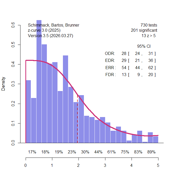
An alternative approach examines false positives for sets of studies rather than a single study. The statistical results of original articles are used to estimate the average power of studies and to use power to evaluate the risk of false positive results. One of the first attempts to do so was Button, Ioannidis, Mokrysz, Nosek, Flint, Robinson, and Munafò’s (2013) article “Power failure: why small sample size undermines the reliability of neuroscience.” The key empirical finding was that median power of 730 studies from 49 meta-analysis was 21%. The article did not provide an empirical estimate of the false positive rate, but it did illustrate implications of the power estimate for false positive rates in various scenarios. The authors suggested that “a major implication is that the likelihood that any nominally significant finding actually reflects a true effect is small” (p. 371). This claim has contribute to concerns that many published significant results are unreliable.
Reexamining The Power Failure
More than ten years later, it is possible to revisit the seminal article with the benefit of hindsight. Advances in the estimation of true power have revealed important conceptual problems that are different from the computation of hypothetical power for the purpose of sample size planning (Brunner & Schimmack, 2020; Soto & Schimmack, 2026).
Cohen defined statistical power as the probability of obtaining a significant result (1988). In the context of sample size planning, however, power is defined as the probability of obtaining a significant result given a hypothetical population effect size greater than zero. This conditional definition of power given a true hypothesis is widely used in the power literature and was also used by Ioannidis (2005) in his calculations of false positive rates.
Assuming only true hypothesis to compute power is reasonable for hypothetical scenarios, but not for the estimation of true power of completed studies. As the population effect size remains unknown after a study produced an effect size estimate, it is not possible to assume an effect size greater than zero. Thus, the true probability of a completed study to produce a significant result is unconditional and independent of the distinction between H0 and H1. Any estimate of average true power is therefore an estimate of the unconditional probability to produce a significant result. This average can contain tests of true null-hypothesis.
The distinction between conditional and unconditional probabilities has important implications for Button’s calculations of false positive rates. The median power of 21% is unconditional, but the false positive calculations assume conditional power. This can lead to inflated estimates of false positive rates. For example, mean power of 20% could be made up of 50% true H0 with a 5% probability to produce a (false) significant results and 50% tests of H1 with 35% power. In this scenario, the false positive rate is 2.5% / (2.5% + 17.5) = 12.5%. Increasing the proportion of true hypothesis that were tested to a 4:1 ratio would increase the conditional power of tests of H1 to 80% to maintain 20% average power. The false positive rate would increase to .04 / (.04 + .15) = 20%. As noted by Soric (1989), we can even compute the maximum false positive rate that is consistent with unconditional mean power assuming conditional power of 1. With mean power of 21%, the maximum ratio of H0 over H1 is 5.25:1 and the maximum false discovery rate is 20%.
Table 1
Maximum False Discovery Rate for 20% Unconditional Power (Soric, 1989)
Not Significant
Significant
Total
H₁ True
.000
.160
.160
H₀ True
.798
.042
.840
Total
.798
.202
1.000
H₀ : H₁ Ratio
5.25 : 1
False Discovery Rate
.208
Note. The table shows the maximum false discovery rate when average unconditional power equals 20%. This maximum occurs when conditional power for true hypotheses (H₁) equals 100%. The false discovery rate equals the proportion of significant results that are false positives: .042 / .202 = .208. Any lower conditional power with the same unconditional power of 20% produces a lower false discovery rate.
The 21% false positive rate overestimates the true false positive rate with 21% median power for two reasons. Soric’s formula assumes that H1 are tested with 100% power. Assuming that many tests of small true effect sizes in small samples have low conditional power, the true false positive rate is below 21%. The second reason is that unconditional power has a skewed distribution with many low power studies and a few high power studies. As a result, mean power will be higher than median power. Button et al.’s provide information about mean power based on their analyses of publication bias that uses mean power. This analysis suggested that 254 of the 730 studies were expected to produce a significant result and the expected percentage of significant results is equivalent to mean power (Brunner & Schimmack, 2020). Thus, mean power was estimated to be 254 / 730 = 35%. Based on Soric’s formula, the maximum false discovery rate with 35% significant results is 10%.
In conclusion, Button et al.’s estimate of unconditional mean power can be used to draw inferences about false positives in the meta-analyses that they examined that do not rely on unknown ratios of true and false hypotheses being tested in neuroscience. Using their data and Soric’s formula suggests that the false positive risk is fairly small.
A Z-Curve Analyses of Button et al.’s Data
Button et al.’s article contribute to a culture of open sharing of data, but that was not the norm when the article was published. Fortunately, Nord et al. (2017) conducted further analyses of the data and shared power estimates for the 730 studies in an Open Science Foundation (OSC) project. The power estimates do not use the effect sizes of individual studies. Rather they use the sample sizes and the meta-analytic effect size to estimate power. This approach corrects for effect size inflation in smaller studies and reduces bias in power estimates. The following analyses used these data. Power estimates based on individual studies are likely to be inflated by publication bias.
Based on these data, 28% of the studies were statistically significant. Mean power was 35%, matching Button et al.’s estimate of mean power, suggesting that Nord et al.’s power values are based on meta-analytic effect sizes.
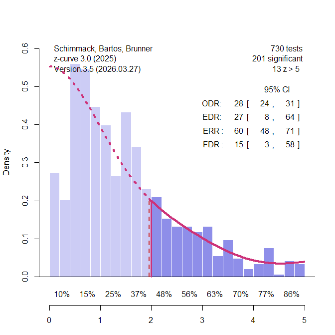
I converted power values into z-values and analyzed the z-values with z-curve.3.0 using the default model (Figure 1).
The observed discovery rate (ODR) is simply the percentage of significant results. More important is the bias-corrected estimate of unconditional mean power for all 730 z-values. Z-curve uses the observed distribution of significant z-values and projects the fitted model into the range of unobserved significant results. As shown in Figure 1, the model predicts the actual distribution of non-significant results fairly well. This suggests that the use of meta-analytic effect sizes adjusted inflated effect size estimates and removed publication bias. The estimated mean power for all studies is called the expected discovery rate (EDR). The EDR estimate is close to the ODR, suggesting further that the data are unbiased.
A key problem of estimating the EDR based on the significant results only is that the confidence interval around the point estimate is very wide. When the data show no major bias, more precise estimates can be obtained by fitting the model to all 730 data (Figure 2).
The key finding is that the point estimate of the false positive risk, FDR = 13% is in line with calculations based on Button’s estimate of mean power. The confidence interval around this estimate limits the FDR at 20%. This is an upper limit because conditional power of studies with significant results is likely to be less than 100%.
In fact, z-curve makes it possible to estimate conditional power of significant studies. First, z-curve estimates unconditional average power of significant studies. This parameter is called the expected replication rate (ERR) because it predicts how many studies would produce a significant result again in a hypothetical replication project that reproduces the original studies exactly with new samples. The ERR is 54% with an upper limit of 60% for the 95% confidence interval. We also know that no more than 20% of these studies are false positives. Assuming 80% true hypotheses, the average conditional power can not be higher than (.60 – .20*.05) / .8 = 74%. Thus, Soric’s assumption of 100% power is conservative, and the false positive rate is likely to be lower.
In conclusion, a z-curve analysis of Nord et al.’s power estimates for Button et al.’s meta-analyses confirms estimates that could have been obtained by applying Soric’s formula to Button et al.’s estimate of mean power. The true rate of false positive results remains unknown, but it is unlikely to be more than 20%.
Heterogeneity Across Research Areas
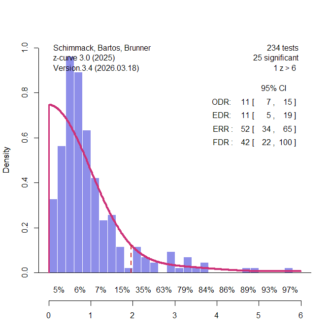
Nord et al. (2017) demonstrated that power varies across different research areas that were included in Button et al.’s sample of meta-analyses. Some of these areas had enough studies to conduct z-curve analyses for these specific areas. The most interesting area are candidate-gene studies that relate genotypic variation in single genes to phenotypes across participants With the benefit of hindsight, it is known that variation in a single gene has trivial effects on complex traits and that many of the significant results in these studies were practically false positive results (Duncan & Keller, 2011). 234 of the 730 studies were from this research area. Figure 3 shows the results. Interestingly, only 11% of the results were statistically significant. Thus, the low average power can be explained by many studies that reported non-significant results. There is no evidence of publication bias in these meta-analyses.
Using Soric’s formula, the low EDR translates into a high false positive risk, 42% and the upper limit of the 95% confidence interval includes 100%. Thus, z-curve confirms that the rare significant results in this literature could be false positive results. Most significant results also are just significant. There are hardly any results that show strong evidence (z > 4) against the null-hypothesis.
In short, a large portion of the 730 studies came from a research area that is known to have produced few significant results. This finding implies that other research areas are producing more credible significant results (Nord et al., 2017).
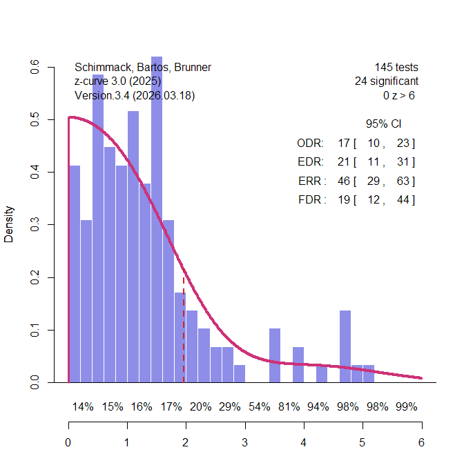
A second set of meta-analyses were clinical trials. Clinical trials have received considerable attention using Cochrane meta-analyses and abstracts in original articles that often report the key statistical result ( (Jager & Leek, 2013; Schimmack & Bartos, 2023, van Zwet et al., 2024). The results suggest that unconditional mean power is around 30% and the false positive risk is between 10% and 20%. These results serve as benchmarks for the z-curve analysis of the 145 clinical trials in Button et al.’s study (Figure 4).
The EDR is somewhat lower, 21%, but the 95% confidence interval includes 30%. The FDR is 19%, but the lower limit of the confidence interval includes 13%. Thus, the results are a bit lower, but mostly consistent with evidence from estimates based on thousands of results. These estimates of the FDR are notably lower than the false positive rates that were predicted by Ioannidis’s scenarios that assumed high rates of true null-hypotheses.
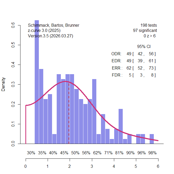
The third domain were studies from psychology. Psychological scientists have examined the credibility of their research in the wake of replication failures (Open Science Collaboration, 2015). Suddenly, only significant results in multiple studies within a single study were no longer attributed to reliable effects, but seen as signs of selection for significance (Schimmack, 2012). Francis (2014) found that over 80% of these multi-study articles showed statistically significant evidence of bias. Large scale multi-lab replication studies failed also showed that effect sizes estimates in these studies could be inflated by a factor of 1,000, shrinking effect sizes from d = .6 to d = .06 (Vohs et al., 2019). A z-curve analysis of a representative sample of studies in social psychology estimated that average unconditional power before selection for significance, EDR = 19%, FDR = 22%. Cohen (1962) already found similar estimates are similar for focal and non-focal results. This was also the case in a survey of emotion research (Soto & Schimmack, 2024). Soto and Schimmack (2024) reported an EDR of 30% and a corresponding FDR = 12% (k sig = 21,628) for all automatically extracted tests, and an EDR of 27%, FDR = 14%, for hand-coded focal tests (k sig = 227). These results serve as a comparison standard for the z-curve of 145 studies classified as psychological research by Nord et al. (2017). The EDR is 49%, FDR = 5%. Even the lower limit of the EDR confidence interval, 39%, implies only 8% false positives. among the significant results.
There are several reasons why these results differ from other findings. First, the focus on meta-analyses leads to an unrepresentative sample of the entire literature. Meta-analyses often include a lot more non-significant results and have less bias than original articles. Second, the specific set of meta-analyses was not representative of the broader literature in psychology. Thus, the results cannot be generalized from the specific studies in Button et al.’s sample to psychology or neuroscience. That would require representative sampling or collecting data from all studies using automatic extraction of test statistics.
Discussion
Button et al.’s (2013) was a first attempt to assess the credibility of empirical results with empirical estimates of power based on meta-analytic effect sizes and sample sizes. The median power was low (21%). The key implications of these finding was that researchers often fail to reject null-hypotheses and may use questionable research practices to report significant results in published articles. Low power and bias could lead to many false positive results. This article added to other concerns about the reliability of findings in neuroscience (Vul et al., 2019).
Most citations took Button et al.’s findings and implications at face value. Nord et al. (2017) pointed out that power and false positive rates varied across research areas. Most notably, candidate gene studies have lower power and a much higher false positive risk. Including these studies in the calculation of median power may have led to false perceptions of other research areas.
Here I presented the first serious critical examination of Button et al.’s methodology and inferences and found several problems that undermine their pessimistic assessment of neuroscience. First, they estimated unconditional power, but their false positive calculations require estimates of conditional power. Second, false positives rates depend on mean power and not median power. Mean power was 35% which is close to the estimate for psychology based on actual replication studies (OSC, 2015). Third, they made unnecessary assumptions about ratios of true and false hypotheses being tested, when unconditional power alone is sufficient to estimate false positive rates (Soric, 1989). Fourth, they relied on meta-analysis to correct for publication bias, but meta-analyses are not representative of the broader literature.
Meta-science is like other sciences. Ideally, critical analyses reveal problems and new innovations address these problems. Power estimation started in the 1960s with Cohen’s seminal article. Cohen (1962) worked with plausible effect sizes, but did not aim to estimate studies true power. Moreover, his work and statistical power were largely ignored (Cohen, 1990; Sedlmeier & Gigenzer, 1989).
Conclusion
The replication crisis stimulated renewed interest in methods that use observed results to draw inferences about the power of actual studies (Ioannidis & Trikalinos, 2007; Francis, 2014; Schimmack, 2012; Simonsohn, Nelson, & Simmons, 2014). This work shifted attention from prospective power calculations to the retrospective assessment of evidential strength in published literatures. Two challenges emerged as central. First, selection bias inflates the observed rate of significant results, requiring methods that correct for selection. Second, power varies across studies, requiring models that allow for heterogeneity rather than assuming a single common effect size or power level. Early approaches addressed selection under simplifying assumptions, typically treating power as homogeneous across studies. As a result, their inferences become unreliable when studies differ in sample size, effect size, or both (Brunner & Schimmack, 2020; Schimmack, 2026).
Z-curve extends this line of work by explicitly modeling both selection and heterogeneity, estimating a distribution of power across studies rather than a single average. This provides a framework for quantifying key properties of the literature, including expected discovery and replication rates, and for linking these quantities to false discovery risk (Sorić, 1989). In this sense, z-curve represents a substantive advance in the empirical assessment of the credibility of published findings. Like earlier contributions such as Button et al., it is unlikely to be the final word, but it is currently the most advanced method to estimate true power for sets of studies with heterogeneity in power and selection bias.
P-curve is a statistical tool that was designed to evaluate the statistical credibility of significant results. When only significant results are published, it is unclear how much selection for significance contributed to the results. In the worst case scenario, all published results are false positives. P-curve uses a variety of approaches to test this worst case scenario. If the null-hypothesis can be rejected, the data are said to have evidential value; that is, at least some of the studies rejected a false null-hypothesis.
P-curve was published without extensive validation research. Critical examination of the method has focussed on the estimate of average power (Brunner, 2018; Brunner & Schimmack, 2020). Average power can quantify the strength of evidence against the null-hypothesis rather than simply rejecting the null-hypothesis of no evidence. For example, a set of studies could have 18% average power, suggesting that some significant results were true positives, but also showing that this literature has many studies with low power.
The problem with p-curve is that, contrary to claims by its developer, it produces inflated estimates of power when studies vary in power. For example, it predicts that 91% of replications should have been successful in the reproducibility project (Open Science Collaboration, 2015), when only 36% of the actual replications were successful. This bias is expected given the large heterogeneity in power across these studies (Schimmack & Soto, 2026). A solution to this problem is to use z-curve (Bartos & Schimmack, 2022; Brunner & Schimmack, 2020). Z-curve is explicitly designed for heterogenous data and performs well with low and high heterogeneity (Schimmack & Soto, 2026).
Morey and Davis-Stober (2025) raised further concerns about the statistical properties of p-curve. Given the similar aims of p-curve and z-curve, it is reasonable to wonder whether z-curve suffers from some of the same problems as p-curve, despite its ability to handle heterogeneity well. I asked Claude AI to examine this question and it concluded that z-curve is built on a fundamentally different approach than p-curve that avoids many of p-curve’s pitfalls. Here is a summary of the evaluation.
Not applicable — z-curve targets power, not effect size
P-curve’s problems go beyond heterogeneity
The most fundamental problem is inadmissibility of the core test of evidential value (EV). The core test — the version currently in the p-curve app — uses a probit transformation that produces a concave acceptance region in the test statistic space. By results from Birnbaum (1954) and Marden (1982), this makes the test inadmissible: its power is dominated by other tests for every possible alternative, including the homogeneous case. The 2015 switch from the log to the probit transformation was motivated by wanting robustness to extreme values, but admissibility requires exactly the property that was engineered out — sensitivity to large individual test statistics.
The compound half p-curve rule introduces nonmonotonicity: increasing the evidence in a single study can flip the procedure from rejection to acceptance and back, multiple times, along a monotonically increasing path. This is a purely structural consequence of the hard boundary at αpc/2 combined with the probit transform, and has nothing to do with whether effect sizes are heterogeneous.
Test LEV, which is supposed to detect “lack of evidential value,” has an additional pathology: arbitrarily large test statistics contribute zero weight to the sum, because they map to log(1) = 0. A single study with a p value just below 0.05 can dominate the test and force rejection regardless of how large every other test statistic is. Six studies with Z = ∞ plus one study at Z = 1.97 yields the same test statistic as six studies at Z = 1.97.
None of these problems affect z-curve. Z-curve uses EM estimation on a mixture of truncated normal distributions, fitting the full shape of the observed z-score distribution above the significance threshold. Large z-scores contribute information proportional to their posterior weight on high-NCP components. The EM likelihood surface is smooth and does not blow up near the truncation boundary. There is no compound decision rule. And because z-curve’s target quantities are replicability (ERR) and discovery rate (EDR) — both functions of noncentrality parameters — there is no conflation of power with effect size.
The Morey and Davis-Stober paper does not mention z-curve. It does not need to. Their formal results simply confirm, from a different direction and with different tools, what simulation studies have shown for years: p-curve’s statistical machinery is not up to the job it advertises. Z-curve was designed from the start to avoid exactly these pitfalls.
In short, z-curve is not just another p-curve. While the aims are similar, the statistical approach and the ability to handle realistic amounts of heterogeneity are very different. Morey and Davis-Stober’s critique is limited to p-curve and does not generalize to z-curve.
Full citation: Soto, M. D., & Schimmack, U. (2024). Credibility of results in emotion science: A Z-curve analysis of results in the journals Cognition & Emotion and Emotion. Cognition and Emotion. https://doi.org/10.1080/02699931.2024.2443016
Purpose of this document: This is a detailed analytical summary written entirely in the summarizer’s own words. It is intended to make the paper’s methods, results, and arguments accessible for discussion and analysis without reproducing copyrighted text. Readers should consult the original article for exact language and figures.
Structured Summary
1. Motivation and Research Question
The paper addresses whether the replication crisis — documented most prominently by the Open Science Collaboration (2015), which found only 36% of psychology results replicated — extends to the emotion research literature specifically. The authors note that the OSC findings were limited to articles from 2008 and may not generalize to emotion research, which has its own dedicated journals and traditions.
The two journals examined are Cognition & Emotion (established 1987) and Emotion (established 2001 by APA). The authors aimed to assess: (a) how much selection bias exists in these journals, (b) what proportion of published results might be false positives, (c) what the expected replication rate is, and (d) whether these indicators have improved over time in response to the replication crisis.
2. Z-Curve Method: How It Works
The paper uses Z-curve 2.0 (Bartoš & Schimmack, 2022), which takes a set of test statistics, converts them to absolute z-scores, and fits a finite mixture model to the distribution of statistically significant z-values (those exceeding 1.96). The method produces four key estimates:
Expected Discovery Rate (EDR): An estimate of the average true power of studies before selection for significance. This represents what proportion of all conducted tests (including unpublished ones) would be expected to reach significance. It is conceptually the mean power across the full population of tests.
Expected Replication Rate (ERR): An estimate of mean power after selection for significance — that is, among published significant results. Because significance selection favors higher-powered studies, ERR is always higher than EDR. The authors frame ERR as an optimistic upper bound on expected replication success.
Observed Discovery Rate (ODR): Simply the proportion of extracted test statistics that were statistically significant at p < .05. Comparing ODR to EDR quantifies selection bias: a large gap indicates that many non-significant results went unreported.
False Discovery Risk (FDR): Computed from the EDR using Soric’s (1989) formula, which gives the maximum proportion of significant results that could be false positives given a particular discovery rate.
The authors explicitly note that ERR overestimates actual replication success (comparing z-curve’s ERR for the OSC dataset to the actual 36% rate), and they recommend interpreting the true replication rate as falling somewhere between EDR and ERR, citing Sotola (2023) for empirical support.
3. Methods
3.1 Test Statistic Extraction
The authors collected the complete set of published articles from both journals (3,831 from C&E covering 1987–2023; 2,323 from Emotion covering 2001–2023). Using custom R code built on the pdftools package (Ooms, 2024), they automatically extracted reported test statistics: F-tests, t-tests, chi-square tests (with df between 1 and 6 only, to exclude SEM model-fit tests), z-tests, and 95% confidence intervals of odds ratios and regression coefficients.
Chi-square tests with df > 6 were excluded because these typically come from structural equation modeling, where rejecting the null indicates poor model fit rather than a substantive finding. Confidence intervals were excluded when reported alongside test statistics to avoid double-counting. Meta-analysis articles were excluded entirely.
The extraction code was designed to handle various notation formats across journals and was iteratively refined. However, the authors acknowledge that the automated process cannot extract statistics from tables or figures, and cannot distinguish between focal and non-focal hypothesis tests.
After exclusions (including test statistics with N < 30, since t-to-z conversion is unreliable at very low df), the final samples were 30,513 z-scores from 1,902 C&E articles and 35,457 z-scores from 1,953 Emotion articles. The majority were F-tests (62% C&E, 53% Emotion) and t-tests (26% C&E, 28% Emotion).
3.2 Statistical Analysis — The Clustering Approach
This is a critical methodological detail. The authors used the zcurve_clustered function with the “b” method. This method works by sampling a single test statistic from each article during model fitting, thereby addressing within-article dependence. This directly addresses concerns about independence violations that arise when multiple test statistics are extracted from the same paper.
The EM algorithm was applied to significant z-values between 1.96 and 6 (values above 6 are treated as having essentially 100% power). The fitted mixture model uses seven discrete components (z = 0 through 6), and the estimated weights are used to compute EDR and ERR. The model then extrapolates the full distribution to estimate what the non-significant portion would look like without selection.
3.3 Time Trend Analysis
Annual z-curve estimates were computed for each publication year and regressed on linear and quadratic predictors of year. The quadratic term tested whether improvements accelerated after 2011 (when the replication crisis became prominent).
3.4 Hand-Coded Focal Tests
To address the limitation that automatic extraction conflates focal and non-focal tests, the authors also present results from 241 hand-coded articles from 2010 and 2020, drawn from an ongoing project covering 30+ journals and 4,000+ studies (Schimmack, 2020). This sample contained 227 significant tests out of 241 total.
4. Results
4.1 Main Z-Curve Estimates
The two journals produced remarkably similar results:
Parameter
Cognition & Emotion
Emotion
ODR
71% [70%, 71%]
70% [70%, 70%]
EDR
30% [14%, 53%]
31% [15%, 53%]
ERR
66% [59%, 73%]
65% [59%, 71%]
FDR
12% [5%, 32%]
12% [5%, 30%]
The ODR-EDR gap (approximately 40 percentage points) provides clear evidence of selection bias in both journals, confirmed visually by a sharp drop in observed z-scores just below the significance threshold of 1.96.
The ERR of approximately 65% suggests that the majority of published significant results should replicate with the same sample size, though the authors stress this is an optimistic estimate. The FDR point estimate of 12% is comparable to medical clinical trial journals (14% per Schimmack & Bartoš, 2023) and substantially lower than the most pessimistic predictions (Ioannidis, 2005). However, the upper bound of the FDR confidence interval (~30%) is high enough to warrant concern.
4.2 Time Trends
Sample sizes (degrees of freedom): Both journals showed significant linear increases over time, with some acceleration (significant quadratic trends). Median within-group df increased from roughly 50 in the early years to over 100 in recent years for Emotion, and showed a particularly sharp increase in C&E’s most recent years.
ODR: Both journals showed significant linear decreases in ODR over time (approximately 0.45 percentage points per year), suggesting that non-significant results are being reported more frequently. However, the quadratic terms were non-significant, meaning this trend preceded the replication crisis rather than being a response to it.
EDR: Both journals showed significant increases in EDR over time, consistent with increasing sample sizes leading to higher power. The combination of decreasing ODR and increasing EDR indicates that selection bias has diminished, though it remains present.
ERR: Increased over time for both journals, with C&E showing a significant acceleration (quadratic trend) suggesting the replication crisis may have prompted improvements.
FDR: Decreased over time as a direct consequence of the increasing EDR.
4.3 Hand-Coded Focal Test Results
The 241 hand-coded focal tests from 2010 and 2020 yielded:
Parameter
Estimate
95% CI
ODR
94%
[91%, 97%]
EDR
27%
[10%, 67%]
ERR
65%
[53%, 75%]
FDR
14%
[3%, 50%]
The ODR for focal tests (94%) is substantially higher than the 70–71% from automatic extraction, confirming that automatic extraction captures many non-focal, non-significant tests that dilute the ODR. However, the EDR, ERR, and FDR estimates are comparable to the automatically extracted results and fall within their confidence intervals. This is an important robustness check: the key z-curve parameters are not substantially altered by the inclusion of non-focal tests.
4.4 Alpha Adjustment Analysis
The authors examined the effect of lowering the significance threshold on discovery rates and false positive risk. Lowering alpha from .05 to .01 retains approximately half of all significant results while reducing FDR to below 5% for most publication years. Further reductions to .005 or .001 have diminishing returns for FDR reduction but increasingly sacrifice power.
5. Discussion and Interpretation
The authors frame their results as relatively encouraging for emotion research compared to worst-case scenarios. Key interpretive points:
The FDR of approximately 12% (though with wide CIs) suggests that most published significant results in emotion journals are not false positives. However, the upper bound of the CI leaves open the possibility of rates up to 30%.
The ERR of 65% predicts that most significant results should replicate with the same sample size, but this is optimistic. Adjusting for the estimated FDR, power for true effects may be approximately 72%, close to the conventional 80% benchmark but with substantial heterogeneity — half of studies have less power than this average.
The authors recommend treating results with p-values between .05 and .01 with skepticism, and suggest that alpha = .01 provides a better balance between false positive risk and power loss for the emotion literature specifically. They emphasize this recommendation is for evaluating existing literature, not as a new publication standard.
On effect sizes, the authors warn that selection bias inflates point estimates, making even meta-analytic effect sizes unreliable unless bias correction is applied. They advocate for honest reporting of all results, including non-significant ones, as essential for accurate meta-analysis.
6. Limitations Acknowledged by the Authors
The authors explicitly discuss several limitations:
Z-curve’s selection model assumes that publication probability is a function of power. In reality, questionable research practices (QRPs) can produce significance without real effects, potentially inflating EDR estimates and underestimating selection bias.
Simulation studies of z-curve performance under QRP-generated data are lacking.
The N > 30 exclusion removes some studies, though supplementary analyses with the full sample show similar results.
Automated extraction cannot distinguish focal from non-focal tests (addressed by the hand-coded analysis).
The automated extraction cannot reliably capture statistics from tables or figures.
7. Key Methodological Features Relevant to the Pek et al. Debate
Several aspects of this paper are directly relevant to criticisms raised by Pek et al.:
Independence assumption: Soto & Schimmack explicitly used zcurve_clustered with the “b” method, which samples one test statistic per article during bootstrapping. This directly addresses the concern about within-article dependence. The method section states this clearly.
Focal vs. non-focal tests: The paper includes both automatic extraction (all tests) and hand-coded focal tests, and shows that the z-curve parameters (EDR, ERR, FDR) are comparable across both approaches. This addresses the concern that including non-focal tests distorts results.
Appropriate caveats: The authors consistently describe ERR as optimistic, characterize the true replication rate as lying between EDR and ERR, acknowledge the wide confidence intervals on EDR and FDR, and explicitly discuss the limitations of the selection model assumption.
Asymmetric interpretation: The paper notes that z-curve evaluations of credibility are asymmetric — low values raise concerns about a literature, but high values do not guarantee credibility.
8. Summary Table of All Z-Curve Estimates
Analysis
N tests
N sig
ODR
EDR [95% CI]
ERR [95% CI]
FDR [95% CI]
C&E (auto)
30,513
21,628
71%
30% [14%, 53%]
66% [59%, 73%]
12% [5%, 32%]
Emotion (auto)
35,457
24,824
70%
31% [15%, 53%]
65% [59%, 71%]
12% [5%, 30%]
Focal (hand-coded)
241
227
94%
27% [10%, 67%]
65% [53%, 75%]
14% [3%, 50%]
Summary prepared for analytical discussion purposes. All descriptions reflect the summarizer’s interpretation of the original work. For exact language, figures, and supplementary analyses, consult the published article.
The pattern is now familiar. I received another anonymous review by Reviewer 2 from a z-curve article that repeated Pek’s concerns about the performance of z-curve. To deal with biased reviewers, journals allow authors to mention potentially biased reviewers. I suggest doing so for Pek. I also suggest sharing a manuscript with me to ensure proper interpretation of results and to make it “reviewer-safe.”
To justify the claim that Pek is biased, researchers can use this rebuttal of Pek’s unscientific claims about z-curve.
Reviewer 2
Reviewer Report:
The manuscript “A review and z-curve analysis of research on the palliative association of system justification” (Manuscript ID 1598066) extends the work of Sotola and Credé (2022), who used Z-curve analysis to evaluate the evidential value of findings related to system justification theory (SJT). The present paper similarly reports estimates of publication bias, questionable research practices (QRPs), and replication rates in the SJT literature using Z-curve. Evaluating how scientific evidence accumulates in the published literature is unquestionably important.
However, there is growing concern about the performance of meta-analytic forensic tools such as p-curve (Simonsohn, Nelson, & Simmons, 2014; see Morey & Davis-Stober, 2025 for a critique) and Z-curve (Brunner & Schimmack, 2020; Bartoš & Schimmack, 2022; see Pek et al., in press for a critique). Independent simulation studies increasingly suggest that these methods may perform poorly under realistic conditions, potentially yielding misleading results.
Justification for a theory or method typically requires subjecting it to a severe test (Mayo, 2019) – that is, assuming the opposite of what one seeks to establish (e.g., a null hypothesis of no effect) and demonstrating that this assumption leads to contradiction. In contrast, the simulation work used to support Z-curve (Brunner & Schimmack, 2020; Bartoš & Schimmack, 2022) relies on affirming belief through confirmation, a well-documented cognitive bias.
Findings from Pek et al. (in press) show that when selection bias is presented in published p-values — the very scenario Z-curve was intended to be applied — estimates of the expected discovery rate (EDR), expected replication rate (ERR), and Sorić’s False Discovery Risk (FDR) are themselves biased.
The magnitude and direction of this bias depend on multiple factors (e.g., number of p-values, selection mechanism of p-values) and cannot be corrected or detected from empirical data alone. The manuscript’s main contribution rests on the assumption that Z-curve yields reasonable estimates of the “reliability of published studies,” operationalized as a high ERR, and that the difference between the observed discovery rate (ODR) and EDR quantifies the extent of QRPs and publication bias.
The paper reports an ERR of .76, 95% CI [.53, .91] and concludes that research on the palliative hypothesis may be more reliable than findings in many other areas of psychology. There are several issues with this claim. First, the assertion that Sotola (2023) validated ERR estimates from the Z-curve reflects confirmation bias – I have not read Röseler (2023) and cannot comment on the argument made in it. The argument rests solely on the descriptive similarly between the ERR produced by Z-curve and the replication rate reported by the Open Science Collaboration (2015). However, no formal test of equivalence was conducted, and no consideration was given to estimate imprecision, potential bias in the estimates, or the conditions under which such agreement might occur by chance.
At minimum, if Z-curve estimates are treated as predicted values, some form of cross-validation or prediction interval should be used to quantify prediction uncertainty. More broadly, because ERR estimates produced by Z-curve are themselves likely biased (as shown in Pek et al., in press), and because the magnitude and direction of this bias are unknown, comparisons about ERR values across literatures do not provide a strong evidential basis for claims about the relative reliability of research areas.
Furthermore, the width of the 95% CI spans roughly half of the bounded parameter space of [0, 1], indicating substantial imprecision. Any claims based on these estimates should thus be contextualized with appropriate caution.
Another key result concerns the comparison of EDR = .52, 95% CO [.14, .92], and ODR = .81, 95% CI = [.69, .90]. The manuscript states that “When these two estimates are highly discrepant, this is consistent with the presence of questionable research practices (QRPS) and publication bias in this area of research (Brunner & Schimmack, 2020).
But in this case, the 95% CIs for the EDR and ODR in this work overlapped quite a bit, meaning that they may not be significantly different…” (p. 22). There are several issues with such a claim. First, Z curve results cannot directly support claims about the presence of QRPs.
The EDR reflects the proportion of significant p values expected under no selection bias, but it does not identify the source of selection bias (e.g., QRPs, fraud, editorial decisions). Using Z curve requires accepting its assumed missing data mechanism—a strong assumption that cannot be empirically validated.
Second, a descriptive comparison between two estimates cannot be interpreted as a formal test of difference (e.g., eyeballing two estimates of means as different does not tell us whether this difference is not driven by sampling variability). Means can be significantly different even if their confidence intervals overlap (Cumming & Finch, 2005).
A formal test of the difference is required. Third, EDR estimates can be biased. Even under ideal conditions, convergence to the population values requires extremely large numbers of studies (e.g., > 3000, see Figure 1 of Pek et al., in press).
The current study only has 64 tests. Thus, even if a formal test of the difference of ODR – EDR was conducted, little confidence could be placed on the result if the EDR estimate is biased and does not reflect the true population value.
Although I am critical of the outputs of Z curve analysis due to its poor statistical performance under realistic conditions, the manuscript has several strengths. These include adherence to good meta analytic practices such as providing a PRISMA flow chart, clearly stating inclusion and exclusion criteria, and verifying the calculation of p values. These aspects could be further strengthened by reporting test–retest reliability (given that a single author coded all studies) and by explicitly defining the population of selected p values. Because there appears to be heterogeneity in the results, a random effects meta analysis may be appropriate, and study level variables (e.g., type of hypothesis or analysis) could be used to explain between study variability. Additionally, the independence of p values has not been clearly addressed; p values may be correlated within articles or across studies. Minor points: The “reliability” of studies should be explicitly defined. The work by Manapat et al. (2022) should be cited in relation to Nagy et al. (2025). The findings of Simmons et al. (2011) applies only to single studies.
However, most research is published in multi-study sets, and follow-up simulations by Wegener at al. (2024) indicate that the Type I error rate is well-controlled when methodological constraints (e.g., same test, same design, same measures) are applied consistently across multiple studies – thus, the concerns of Simmons et al. (2011) pertain to a very small number of published results.
I could not find the reference to Schimmack and Brunner (2023) cited on p. 17.
Rebuttal to Core Claims in Recent Critiques of z-Curve
1. Claim: z-curve “performs poorly under realistic conditions”
Rebuttal
The claim that z-curve “performs poorly under realistic conditions” is not supported by the full body of available evidence. While recent critiques demonstrate that z-curve estimates—particularly EDR—can be biased under specific data-generating and selection mechanisms, these findings do not justify a general conclusion of poor performance.
Z-curve has been evaluated in extensive simulation studies that examined a wide range of empirically plausible scenarios, including heterogeneous power distributions, mixtures of low- and high-powered studies, varying false-positive rates, different degrees of selection for significance, and multiple shapes of observed z-value distributions (e.g., unimodal, right-skewed, and multimodal distributions). These simulations explicitly included sample sizes as low as k ≈ 100, which is typical for applied meta-research in psychology.
Across these conditions, z-curve demonstrated reasonable statistical properties conditional on its assumptions, including interpretable ERR and EDR estimates and confidence intervals with acceptable coverage in most realistic regimes. Importantly, these studies also identified conditions under which estimation becomes less informative—such as when the observed z-value distribution provides little information about missing nonsignificant results—thereby documenting diagnosable scope limits rather than undifferentiated poor performance.
Recent critiques rely primarily on selective adversarial scenarios and extrapolate from these to broad claims about “realistic conditions,” while not engaging with the earlier simulation literature that systematically evaluated z-curve across a much broader parameter space. A balanced scientific assessment therefore supports a more limited conclusion: z-curve has identifiable limitations and scope conditions, but existing simulation evidence does not support the claim that it generally performs poorly under realistic conditions.
2. Claim: Bias in EDR or ERR renders these estimates uninterpretable or misleading
Rebuttal
The critique conflates the possibility of bias with a lack of inferential value. All methods used to evaluate published literatures under selection—including effect-size meta-analysis, selection models, and Bayesian hierarchical approaches—are biased under some violations of their assumptions. The existence of bias therefore does not imply that an estimator is uninformative.
Z-curve explicitly reports uncertainty through bootstrap confidence intervals, which quantify sampling variability and model uncertainty given the observed data. No evidence is presented that z-curve confidence intervals systematically fail to achieve nominal coverage under conditions relevant to applied analyses. The appropriate conclusion is that z-curve estimates must be interpreted conditionally and cautiously, not that they lack statistical meaning.
This claim overgeneralizes results from specific, highly constrained simulation scenarios. The cited sample sizes correspond to conditions in which the observed data provide little identifying information, not to a general requirement for statistical validity.
In applied statistics, consistency in the limit does not imply that estimates at smaller sample sizes are meaningless; it implies that uncertainty must be acknowledged. In the present application, this uncertainty is explicitly reflected in wide confidence intervals. Small sample sizes therefore affect precision, not validity, and do not justify dismissing the estimates outright.
4. Claim: Differences between ODR and EDR cannot support inferences about selection or questionable research practices
Rebuttal
It is correct that differences between ODR and EDR do not identify the source of selection (e.g., QRPs, editorial decisions, or other mechanisms). However, the critique goes further by implying that such differences lack diagnostic value altogether.
Under the z-curve framework, ODR–EDR discrepancies are interpreted as evidence of selection, not of specific researcher behaviors. This inference is explicitly conditional and does not rely on attributing intent or mechanism. Rejecting this interpretation would require demonstrating that ODR–EDR differences are uninformative even under monotonic selection on statistical significance, which has not been shown.
5. Claim: ERR comparisons across literatures lack evidential basis because bias direction is unknown
Rebuttal
The critique asserts that because ERR estimates may be biased with unknown direction, comparisons across literatures lack evidential value. This conclusion does not follow.
Bias does not eliminate comparative information unless it is shown to be large, variable, and systematically distorting rankings across plausible conditions. No evidence is provided that ERR estimates reverse ordering across literatures or are less informative than alternative metrics. While comparative claims should be interpreted cautiously, caution does not imply the absence of evidential content.
6. Claim: z-curve validation relies on “affirming belief through confirmation”
Rebuttal
This characterization misrepresents the role of simulation studies in statistical methodology. Simulation-based evaluation of estimators under known data-generating processes is the standard approach for assessing bias, variance, and coverage across frequentist and Bayesian methods alike.
Characterizing simulation-based validation as epistemically deficient would apply equally to conventional meta-analysis, selection models, and hierarchical Bayesian approaches. No alternative validation framework is proposed that would avoid reliance on model-based simulation.
7. Implicit claim: Effect-size meta-analysis provides a firmer basis for credibility assessment
Rebuttal
Effect-size meta-analysis addresses a different inferential target. It presupposes that studies estimate commensurable effects of a common hypothesis. In heterogeneous literatures, pooled effect sizes represent averages over substantively distinct estimands and may lack clear interpretation.
Moreover, effect-size meta-analysis does not estimate discovery rates, replication probabilities, or false-positive risk, nor does it model selection unless explicitly extended. No evidence is provided that effect-size meta-analysis offers superior performance for evaluating evidential credibility under selective reporting.
Summary
The critiques correctly identify that z-curve is a model-based method with assumptions and scope conditions. However, they systematically extend these points beyond what the evidence supports by:
extrapolating from selective adversarial simulations,
conflating potential bias with lack of inferential value,
overgeneralizing small-sample limitations,
and applying asymmetrical standards relative to conventional methods.
A scientifically justified conclusion is that z-curve provides conditionally informative estimates with quantifiable uncertainty, not that it lacks statistical validity or evidential relevance.
In the 17th century, early telescopic observations of Mars suggested that the planet might be populated. Now imagine a study that aims to examine whether Martians are taller than humans. The problem is obvious: although we may assume that Martians exist, we cannot observe or measure them, and therefore we end up with zero observations of Martian height. Would we blame the t-test for not telling us what we want to know? I hope your answer to this rhetorical question is “No, of course not.”
If you pass this sanity check, the rest of this post should be easy to follow. It responds to criticism by Erik van Zwet (EvZ), hosted and endorsed by Andrew Gelman on his blog,
EvZ imagines a scenario in which z-curve is applied to data generated by two distinct lines of research. One lab conducts studies that test only true null hypotheses. While exact effect sizes of zero may be rare in practice, attempting to detect extremely small effects in small samples is, for all practical purposes, equivalent. A well-known example comes from early molecular genetic research that attempted to link variation in single genes—such as the serotonin transporter gene—to complex phenotypes like Neuroticism. It is now well established that these candidate-gene studies produced primarily false positive results when evaluated with the conventional significance threshold of α = .05.
In response, molecular genetics fundamentally changed its approach. Researchers began testing many genetic variants simultaneously and adopted much more stringent significance thresholds to control the multiple-comparison problem. In the simplified example used here, I assume α = .001, implying an expected false positive rate of only 1 in 1,000 tests. I further assume that truly associated genetic predictors—single nucleotide polymorphisms (SNPs)—are tested in very large samples, such that sampling error is small and true effects yield z-values around 6. This is, of course, a stylized assumption, but it serves to illustrate the logic of the critique.
Figure 1 illustrates a situation with 1,000 studies from each of these two research traditions. Among the 1,000 candidate-gene studies, only one significant result is expected by chance. Among the genome-wide association studies (GWAS), power to reject the null hypothesis at α = .001 is close to 1, although a small number (3–4 out of 1,000) of studies may still fail to reach significance.
At this point, it is essential to distinguish between two scenarios. In the first scenario, all 999 non-significant results are observed and available for analysis. If we could recover the full distribution of results—including non-significant ones—we could fit models to the complete set of z-values. Z-curve can, in principle, be applied to such data, but it was not designed for this purpose.
Z-curve was developed for the second scenario. In this scenario, the light-purple, non-significant results exist only in researchers’ file drawers and are not part of the observed record. This situation—selection for statistical significance—is commonly referred to as publication bias. In psychology, success rates above 90% strongly suggest that statistical significance is a necessary condition for publication (Sterling, 1959). Under such selection, non-significant results provide no observable information, and only significant results remain. In extreme cases, it is theoretically possible that all published significant findings are false positives (Rosenthal, 1979), and in some literatures—such as candidate-gene research or social priming—this possibility is not merely theoretical.
Z-curve addresses uncertainty about the credibility of published significant results by explicitly conditioning on selection for significance and modeling only those results. When success rates approach 90% or higher, there is often no alternative: non-significant results are simply unavailable.
In Figure 1, the light-purple bars represent non-significant results that exist only in file drawers. Z-curve is fitted exclusively to the dark-purple, significant results. Based on these data, the fitted model (red curve), which is centered near the true value of z = 6, correctly infers that the average true power of the studies contributing to the significant results is approximately 99% when α = .001 (corresponding to a critical value of z ≈ 3.3).
Z-curve also estimates the Expected Discovery Rate (EDR). Importantly, the EDR refers to the average power of all studies that were conducted in the process of producing the observed significant results. This conditioning is crucial. Z-curve does not attempt to estimate the total number of studies ever conducted, nor does it attempt to account for studies from populations that could not have produced the observed significant findings. In this example, candidate-gene studies that produced non-significant results—whether published or not—are irrelevant because they did not contribute to the set of significant GWAS results under analysis.
What matters instead is how many GWAS studies failed to reach significance and therefore remain unobserved. Given the assumed power, this number is at most 3–4 out of 1,000 (<1%). Consequently, an EDR estimate of 99% is correct and indicates that publication bias within the relevant population of studies is trivial. Because the false discovery rate is derived from the EDR, the implied false positive risk is effectively zero—again, correctly so for this population.
EvZ’s criticism of z-curve is therefore based on a misunderstanding of the method’s purpose and estimand. He evaluates z-curve against a target that includes large numbers of studies that leave no trace in the observed record and have no influence on the distribution of significant results being analyzed. But no method that conditions on observed significant results can recover information about such studies—nor should it be expected to.
Z-curve is concerned exclusively with the credibility of published significant results. Non-significant studies that originate from populations that do not contribute to those results are as irrelevant to this task as the height of Martians.
Bartoš, F., & Schimmack, U. (2022). Z-curve 2.0: Estimating replication rates and discovery rates. Meta-Psychology, 6, Article e0000130. https://doi.org/10.15626/MP.2022.2981
Brunner, J., & Schimmack, U. (2020). Estimating population mean power under conditions of heterogeneity and selection for significance. Meta- Psychology. MP.2018.874, https://doi.org/10.15626/MP.2018.874
van Zwet, E., Gelman, A., Greenland, S., Imbens, G., Schwab, S., & Goodman, S. N. (2024). A New Look at P Values for Randomized Clinical Trials. NEJM evidence, 3(1), EVIDoa2300003. https://doi.org/10.1056/EVIDoa2300003
The Story of Two Z-Curve Models
Erik van Zwet recently posted a critique of the z-curve method on Andrew Gelman’s blog.
Meaningful discussion of the severity and scope of this critique was difficult in that forum, so I address the issue more carefully here.
van Zwet identified a situation in which z-curve can overestimate the Expected Discovery Rate (EDR) when it is inferred from the distribution of statistically significant z-values. Specifically, when the distribution of significant results is driven primarily by studies with high power, the observed distribution contains little information about the distribution of nonsignificant results. If those nonsignificant results are not reported and z-curve is nevertheless used to infer them from the significant results alone, the method can underestimate the number of missing nonsignificant studies and, as a consequence, overestimate the Expected Discovery Rate (EDR).
This is a genuine limitation, but it is a conditional and diagnosable one. Crucially, the problematic scenarios are directly observable in the data. Problematic data have an increasing or flat slope of the significant z-value distribution and a mode well above the significance threshold. In such cases, z-curve does not silently fail; it signals that inference about missing studies is weak and that EDR estimates should not be trusted.
This is rarely a problem in psychology, where most studies have low power, the mode is at the significance criterion, and the slope decreases, often steeply. This pattern implies a large set of non-significant results and z-curve provides good estimates in these scenarios. It is difficult to estimate distributions of unobserved data, leading to wide confidence intervals around these estimates. However, there is no fixed number of studies that are needed. The relevant question is whether the confidence intervals are informative enough to support meaningful conclusions.
One of the most powerful set of studies that I have actually seen comes from epidemiology, where studies often have large samples to estimate effect sizes precisely. In these studies, power to reject the null hypothesis is actually not really important, but the data serve as a good example of a set of studies with high power, rather than low power as in psychology.
However, even this example shows a decreasing slope and a mode at significance criterion. Fitting z-curve to these data still suggests some selection bias and no underestimation of reported non-significant results. This illustrates how extreme van Zwet’s scenario must be to produce the increasing-slope pattern that undermines EDR estimation.
What about van Zwet’s Z-Curve Method?
It is also noteworthy that van Zwet does not compare our z-curve method (Bartos & Schimmack, 2022; Brunner & Bartos, 2020) to his own z-curve method that was used to analyze z-values from clinical trials (van Zwet et al., 2024).
The article fits a model to the distribution of absolute z-values (ignoring whether results show a benefit or harm to patients). The key differences between the two approaches are that (a) van Zwet et al.’s model uses all z-values and assumes (implicitly) that there is no selection bias, and (b) that true effect sizes are never zero and errors can only be sign errors. Based on these assumptions, the article concludes that no more than 2% of clinical trials produce a result that falsely rejects a true hypothesis. For example, a statistically significant result could be treated as an error only if the true effect has the opposite sign (e.g., the true effect increases smoking, but a significant result is used to claim it reduced smoking).
The advantage of this method is that it is not necessary to estimate the EDR from the distribution of only significant results, but it does so only by assuming that publication bias does not exist. In this case, we can just count the observed non-significant and significant results and use the observed discovery rate to estimate average power and the false positive risk.
The trade-off is clear. z-curve attempts to address selection bias and sometimes lacks sufficient information to do so reliably; van Zwet’s approach achieves stable estimates by assuming the problem away. The former risks imprecision when information is weak; the latter risks bias when its core assumption is violated.
In the example from epidemiology, there is evidence of some publication bias and omission of non-significant results. Using van Zwet’s model would be inappropriate because it would overestimate the true discovery rate. The focus on sign errors alone is also questionable and should be clearly stated as a strong assumption. It implies that significant results in the right direction are not errors, even if effect sizes are close to zero. For example, a significant result that suggests it extends life is considered a true finding, even if the effect size is one day.
False positive rates do not fully solve that problem, but false positive rates that include zero as a hypothetical value for the population effect size are higher and treat small effects close to zero as errors rather than treating half of them as correct rejections of the null hypothesis. For example, an intervention that decreases smoking by 1% of all smokers is not really different from one that increases it by 1%, but a focus on signs treats only the latter one as an error.
In short, van Zwet’s critique identifies a boundary condition for z-curve, not a general failure. At the same time, his own method rests on a stronger and untested assumption—no selection bias—whose violation would invalidate its conclusions entirely. No method is perfect and using a single scenario to imply that a method is always wrong is not a valid argument against any method. By the same logic, van Zwet’s own method could be declared “useless” whenever selection bias exists, which is precisely the point: all methods have scope conditions.
Using proper logic, we suggest that all methods work when assumptions are met. The main point is to test whether they are met or not. We clarified that z-curve estimation of the EDR assumes that enough low powered studies produced significant results to influence the distribution of significant results. If the slope of significant results is not decreasing, this assumption does not hold and z-curve should not be used to estimate the EDR. Similarly, users of van Zwets first method should first test whether selection bias is present and not use it when it does. They should also examine whether they think a proportion of studies could have tested practically true null hypotheses and not use the method when this is a concern.
Finally, the blog post responds to Gelman’s polemic about our z-curve method and earlier work by Jager and Leek (2014), by noting that Gelman’s critic of other methods exist in parallel to his own work (at least co-authorship) that also modeled distribution of z-values to make claims about power and the risk of false inferences. The assumption of this model that selection bias does not exist is peculiar, given Gelman’s typical writing about low power and the negative effects of selection for significance. A more constructive discussion would apply the same critical standards to all methods—including one’s own.
Cookie Consent
We use cookies to improve your experience on our site. By using our site, you consent to cookies.