Correction (2026-07-14) The original post claimed that violations of the normality assumption biases standard random effects estimates. That finding was based on a coding error in the simulation program. The revised post shows the results for simulations with normal distributed effect sizes for H1 and mixtures of H0 and H1. In these simulations only estimates of the weight-function selection model (weightr package) are biased when the unimodal normal distribution assumption is violated.
Introduction
The main purpose of meta-analysis is to combine the results of quantitative studies. The simplest form averages the effect-size estimates of studies. The average is a better estimate of the population effect size because it draws on the combined sample size of the individual studies, and larger samples have less sampling error. A more sophisticated version takes each study’s sampling error into account, weighting studies with larger samples more heavily than those with smaller samples. This weighted average approximates the estimate one would obtain by pooling the raw data, under the assumption that all studies estimate the same effect.
These so-called fixed-effect meta-analyses assume that the samples are all drawn from the same population and that studies used interchangeable procedures, so that they all estimate a single population effect size. This assumption is defensible for a few phenomena grounded in basic sensory or cognitive architecture. Weber’s law, for instance — that the just-noticeable difference between two stimuli is a roughly constant proportion of their magnitude — reflects a property of sensory transduction and varies little across procedures and individuals. But such near-constants are the exception. Most effects in psychology vary with situational and personality factors, within and across cultures. This variation adds real differences in the true effect sizes across studies, over and above sampling error.
In recognition of this true variation, statisticians developed random-effects models (DerSimonian & Laird, 1986). To model the variation in population effect sizes, it is necessary to select a model that describes the unobserved variation in population effect sizes. From a statistical perspective, the easiest model assumes that population effect sizes have a normal distribution. The symmetry of this assumption implies that the estimate obtained from a set of studies is an unbiased estimate of the true average because positive and negative deviations from the average population effect size cancel each other out, just like random sampling errors cancel each other out.
Distribution Assumptions
From a theoretical perspective, it is unlikely that population effect sizes are normally distributed, particularly when the mean effect is small relative to the between-study heterogeneity. The reason is that effects are typically coded so that positive values are consistent with a directional theoretical prediction (e.g., conflicting colors produce slower responses in the Stroop task). While the size of the effect may vary across studies, it is often implausible that the true effect in some studies would be reversed (that conflicting colors would genuinely speed responses). A normal distribution, however, has support over the entire range of effect sizes and therefore always assigns some probability to negative true effects — an implication that is difficult to justify for a directionally predicted effect. When the mean is small relative to the heterogeneity, a normal distribution implies that a non-trivial proportion of true effects are negative, which is often theoretically implausible.
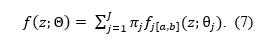
In practice, however, when heterogeneity is small, violations of the normality assumption have small and often negligible effects on meta-analytic estimates of the average effect (Hedges & Vevea, 1996). This helps explain why widely used random-effects models share the assumption that population effect sizes are normally distributed, including standard random-effects meta-analysis (DerSimonian & Laird, 1986) as implemented in commonly used software (Viechtbauer, 2010), selection-model approaches (Vevea & Hedges, 1995; Vevea & Woods, 2005), and the random-effects components of Bayesian model-averaging methods (Bartoš et al., 2023; Maier et al., 2023).
Necessary and Unnecessary Assumptions
It is useful to distinguish between necessary and unnecessary assumptions. All statistical methods require some assumptions to reduce the complex information in data to an interpretable statistic. However, not all assumptions of a model are necessary. In general, models with fewer unnecessary assumptions are preferable because they are robust to violations of these unnecessary assumptions by design. For example, the Pearson correlation coefficient assumes normal distribution of the two variables, whereas rank-order correlations do not. This makes rank-order correlations robust to violations of the normal distribution assumption and it is common practice to prefer rank-order correlations when variables’ distributions are not normal.
In meta-analyses, the assumption that population effect sizes are normally distributed is an unnecessary assumption. The idea of estimating the distribution of effects without assuming a parametric form is not new. Laird (1978) and Lindsay (1983) showed that the mixing distribution in a mixture model can be estimated nonparametrically by maximum likelihood, and that the resulting estimate takes the form of a discrete distribution on a finite set of support points. This provided, in principle, a fully flexible way to model heterogeneity without assuming normality. In practice, however, fitting these models was computationally demanding at the time.
Advances in optimization and computing have since removed these hurdles. Efficient algorithms for estimating mixture models — including modern convex-optimization methods (Koenker & Mizera, 2014; Kim et al., 2020) — now make it possible to fit flexible mixtures quickly and reliably. These developments led to the widespread adoption of nonparametric and empirical-Bayes mixture models in fields that analyze large numbers of effects, most notably genomics (Efron, 2010; Stephens, 2017), where the goal is to characterize the distribution of effects across thousands of tests and to identify which are likely to be real. Similar approaches have been applied in astronomy, education, and other areas that deal with many parallel estimates.
Heterogeneity of Population Effect Sizes
Meta-analysis, however, did not adopt these models, and continued to rely on the normal random-effects model. One reason is that the goal of most meta-analyses has been to estimate a single average effect, for which the shape of the effect-size distribution is largely irrelevant. The additional information provided by a flexible mixture — the structure of the heterogeneity itself — was not part of the question being asked.
This has changed with growing recognition of the distinction between direct and conceptual replication (Zwaan et al., 2018). Experimental psychologists rarely repeat a procedure exactly. Instead, they typically vary paradigms across studies in the belief that this is good scientific practice — probing moderators, boundary conditions, and the generalizability of an effect. As a result, the studies combined in a meta-analysis often estimate genuinely different population effects, and meta-analyses of such conceptual replications frequently show high estimates of heterogeneity (van Erp et al., 2017). In these cases the average effect size is of relatively minor interest, because it merely centers a wide distribution of different population effect sizes — an average across paradigm variants that no single study actually instantiates. The scientifically interesting question is not the average, but how and why the effects differ.
Mixture Models
Mixture models have another advantage over random effects models for meta-analysis. In standard meta-analytic models the population distribution of effect sizes is characterized by the mean and standard deviation of a normal distribution. Importantly, this information is removed from the observed data. It is therefore not possible to use this information to make sense of the heterogeneity in the observed effect size estimates in the data. A large effect size in the data may correspond to a small population effect size because it was inflated by sampling error and vice versa. This explains why heterogeneity often plays a minor role in the interpretation of meta-analyses. Heterogeneity exists, but it cannot be explained.
In contrast, mixture models combined with statistical tools that correct for regression to the mean make it possible to obtain estimates of the population effect size of individual studies. Often these effect size estimates for single studies have large uncertainty (wide confidence intervals), but they can be averaged to identify subgroups of studies with large effect sizes. This makes it possible to explore the heterogeneity in observed studies.
Simulation Study
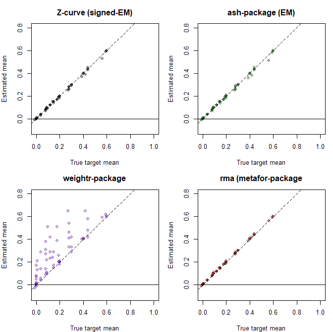
To demonstrate the capabilities and advantages of mixture models over traditional random-effects models, I conducted a simulation study. To isolate the effect of the distributional assumption, the simulation used unbiased data (no publication selection). This removes selection as a confound and allows inclusion of the adaptive-shrinkage mixture model ash (Stephens, 2017), which was developed for genomics and assumes complete, unselected data. The other two models — the weight-function selection model (Vevea & Woods, 2005) and z-curve — model publication bias but reduce to unbiased estimation when no selection is present.
Z-curve is a meta-analytic mixture model (Brunner & Schimmack, 2020; Bartoš & Schimmack, 2022). Version 1 used the noncentrality parameters (ncp) of significant results to estimate the expected replication rate for direct replication studies. Version 2 used the ncp distribution across all studies to estimate the expected discovery rate. Version 3 adds an empirical-Bayes function that estimates population effect sizes by multiplying ncp estimates by their corresponding sampling errors, recovering effects from the latent distribution of noncentrality parameters.
The simulation used fixed sample sizes across studies, which ensures that mixture models fit in the effect-size metric and in the ncp metric produce identical results. Each condition contained k = 1,000 studies; the large k yields small sampling error in the estimates, making systematic biases more visible. The design crossed 4 means and 4 standard deviations of the population effect-size distribution with 4 proportions of true null hypotheses, producing 64 conditions. The population effect sizes when H1 is true were drawn from a normal distribution. However, mixing true H0 and H1 produces non-normal, bimodal distributions. This violates the distribution assumption of standard meta-analytic methods and could produce biased estimates.
These results for the mixture models (z-curve, ash) are not surprising. The models make no distribution assumptions and estimates of the mean closely match the simulated true values (z-curve RMSE = .009; ash RMSE = .010). The weight-function selection model had worse fit (RMSE = .138), but the random effects model fit as well as the mixture models (RMA RMSE = .003).
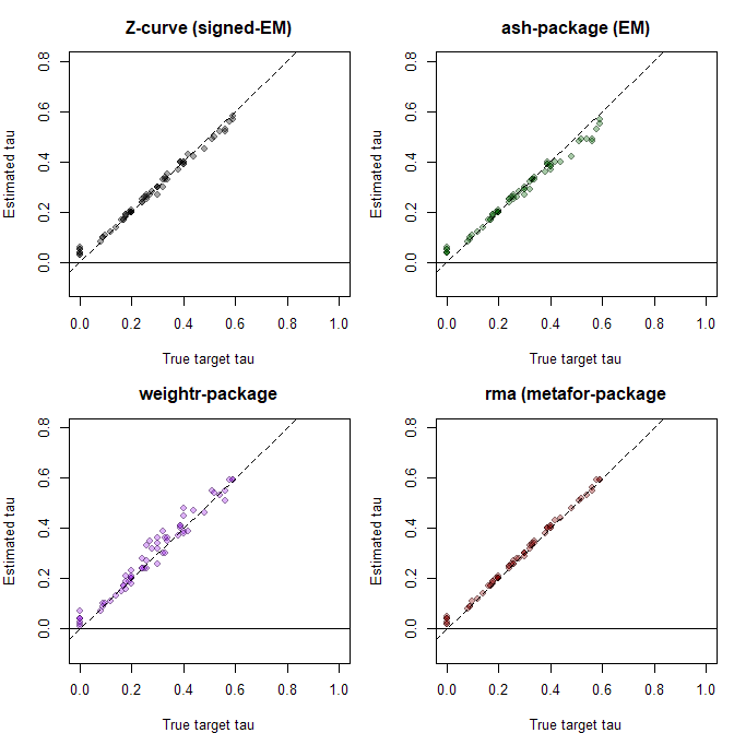
The results for the estimate of heterogeneity (tau) showed that all models estimated heterogeneity well, (z-curve RMSE = .018, ash RMSE = .027, weightr RMSE = .030, RMA RMSE = .013).
The present results show that the random effects model is robust to violations of the normality assumption even when heterogeneity is large and distributions are bimodal. The same cannot be said for the selection model with a normal assumption (weightr). Here the weight parameters to model selection bias can be biased to fit a normal distribution to non-normal observed data. The main implication is that it is possible to improve the performance of selection models by avoiding the normality assumption and modeling the distribution of population effect sizes with a flexible mixture model.
Implications
The present simulation showed that the random-effects model estimates the mean effect well when data are unbiased, even when its distributional assumptions are violated. This is consistent with a substantial prior literature. Simulation studies have repeatedly found that the pooled mean from the normal random-effects model is robust to non-normal random-effects distributions, including skewed and mixture distributions (Yamaguchi et al., 2017; Rubio-Aparicio et al., 2023; Baur et al., 2025). The robustness follows from the estimator itself: the pooled mean is an inverse-variance weighted average, which is consistent for the population mean regardless of the shape of the effect distribution. Large numbers of studies further protect against non-normality (Rubio-Aparicio et al., 2023), and with k = 1,000 the present simulation is in this favorable regime.
Where the normality assumption does matter is not the mean but the characterization of the distribution around it. The same literature finds that non-normality degrades the coverage of confidence and prediction intervals far more than it biases the mean (Baur et al., 2025), and that a symmetric normal model produces a wrongly symmetric prediction interval and a misleading heterogeneity summary when the true distribution is skewed (Yamaguchi et al., 2017). The recognized advantage of flexible mixture and semi-parametric models is therefore not lower bias on the mean but their ability to reveal latent structure — clusters and subgroups of studies — that the mean and a single heterogeneity parameter discard (Baur et al., 2025).
These are real but secondary limitations. The more fundamental problem is one that no distributional flexibility can address: the random-effects model, and the adaptive-shrinkage mixture model (ash) alike, assume that the observed studies are an unbiased sample of the population. In many literatures this assumption is untenable. In psychology, studies with significant results are far more likely to be published; the proportion of significant results often exceeds 90% (Sterling et al., 1995). Such publication bias inflates effect-size estimates, and correcting for it requires modeling the selection process — something neither the random-effects model nor ash attempts. A flexible distribution alone is not enough; what is needed is a model that combines distributional flexibility with a model of selection.
Z-curve occupies this niche: it combines a selection model, which corrects for publication bias, with a flexible mixture model, which captures heterogeneity without a distributional assumption. This is why z-curve outperforms weight-function models when studies are both heterogeneous and affected by publication bias (Schimmack, 2026).
References:
Bartoš, F., Maier, M., Wagenmakers, E.-J., Doucouliagos, H., & Stanley, T. D. (2023). Robust Bayesian meta-analysis: Model-averaging across complementary publication bias adjustment methods. Research Synthesis Methods, 14(1), 99–116.
Böhning, D. (2000). Computer-assisted analysis of mixtures and applications: Meta-analysis, disease mapping and others. Chapman & Hall/CRC.
DerSimonian, R., & Laird, N. (1986). Meta-analysis in clinical trials. Controlled Clinical Trials, 7(3), 177–188.
Hedges, L. V., & Vevea, J. L. (1996). Estimating effect size under publication bias: Small sample properties and robustness of a random effects selection model. Journal of Educational and Behavioral Statistics, 21(4), 299–332.
Laird, N. (1978). Nonparametric maximum likelihood estimation of a mixing distribution. Journal of the American Statistical Association, 73(364), 805–811.
Lindsay, B. G. (1983). The geometry of mixture likelihoods: A general theory. The Annals of Statistics, 11(1), 86–94.
Maier, M., Bartoš, F., & Wagenmakers, E.-J. (2023). Robust Bayesian meta-analysis: Addressing publication bias with model-averaging. Psychological Methods, 28(1), 107–122.
Stephens, M. (2017). False discovery rates: A new deal. Biostatistics, 18(2), 275–294.
Vevea, J. L., & Hedges, L. V. (1995). A general linear model for estimating effect size in the presence of publication bias. Psychometrika, 60(3), 419–435.
Vevea, J. L., & Woods, C. M. (2005). Publication bias in research synthesis: Sensitivity analysis using a priori weight functions. Psychological Methods, 10(4), 428–443.
Viechtbauer, W. (2010). Conducting meta-analyses in R with the metafor package. Journal of Statistical Software, 36(3), 1–48.
Efron, B. (2010). Large-scale inference: Empirical Bayes methods for estimation, testing, and prediction. Cambridge University Press.
Kim, Y., Carbonetto, P., Stephens, M., & Koenker, R. (2020). A fast algorithm for maximum likelihood estimation of mixture proportions using sequential quadratic programming. Journal of Computational and Graphical Statistics, 29(2), 261–273.
Koenker, R., & Mizera, I. (2014). Convex optimization, shape constraints, compound decisions, and empirical Bayes rules. Journal of the American Statistical Association, 109(506), 674–685.
Laird, N. (1978). Nonparametric maximum likelihood estimation of a mixing distribution. Journal of the American Statistical Association, 73(364), 805–811.
Lindsay, B. G. (1983). The geometry of mixture likelihoods: A general theory. The Annals of Statistics, 11(1), 86–94.
To make sense of empirical data, researchers need statistical models, and the choice of model can influence conclusions. It is therefore important to be aware of the assumptions a model makes and, ideally, to test whether those assumptions hold in a particular dataset. This simple truth applies even to the choice of how to describe the average of a variable. As most students learn in a first statistics course, the mean and the median are interchangeable for symmetric distributions but not for skewed ones. In that example, the assumption is easy to check: test the symmetry of the data and pick the better summary.
With more complex models, testing assumptions is harder, and some assumptions cannot be tested at all. In these contexts it is common to leave the influence of assumptions unexamined. It is also awkward to phrase every conclusion as a conditional statement — “assuming the model’s assumptions hold, …” In psychology, correlational researchers are routinely required to flag that any causal claim is conditional on assumptions, or else they are told not to draw conclusions at all. Model-based results, by contrast, are often presented without a careful discussion of the model’s assumptions.
An increasingly popular model for meta-analyses is the step-function selection model (Vevea & Woods, 2005). Like other selection models, it assumes that nonsignificant results often remain unpublished while significant results are published. Other biases may also influence which significant results appear, but most selection models make the simplifying assumption that selection for significance is the key driver of publication bias.
Where selection models differ is in their treatment of nonsignificant results. Models like p-curve and z-curve fit only the significant results and do not condition on the observed nonsignificant ones; they avoid making any assumption about how selection shaped the nonsignificant results. Step-function models instead use the nonsignificant results directly. This can yield more information, but only at the cost of an additional assumption: that the selection process takes a specific form. That extra assumption is the subject of this post — and, as with symmetry and the mean, it is one we can test.
To use non-significant results, step-function models make two assumptions that have to be true to correct for selection bias.
Non-significant and significant effect size estimates come from the same normal distribution of population effect sizes.
Selection bias within a step (a range of p-values) is independent of the p-value.
Taken together, these two assumptions make predictions about the observed p-values within a step. This prediction is easier to test when the p-values are converted into z-values. Essentially, selection bias should influence the frequency of results in a step, but not the shape that one would see without selection bias. This prediction has never been tested, but it is possible to do so using a z-curve plot and z-curve analyses of the data.
Here I use actual data from a meta-analysis of Terror Management Studies that used the step-function model (Chen et al., 2025).
A simple histogram of the z-values shows that there are hardly any negative results (Figure 1). However, Chen et al. specified a model that assumes equal selection bias for all z-values between -1.96 and +1.96. Accordingly, the data imply that there really were more non-significant results with a positive effect than a negative effect. This alone implies that the mean of the population effect sizes is positive. Indeed, the model estimated a mean standardized effect size of .347 standard deviations.
An alternative possibility is that there is a stronger selection bias against negative non-significant results than for positive non-significant results. This assumption can be tested by splitting the step at z = 0 (p = .5, one-tailed) and estimating selection bias separately for positive and negative results. This model produces a dramatically different estimate of the average effect size, suggesting that studies, on average, more often produced a negative result (contrary to predictions) than a positive result, standardized mean difference = -.336.
The change in the sign of the estimate shows how sensitive estimates are to model assumptions. I used z-curve (Brunner & Schimmack, 2020; Bartos & Schimmack, 2022) to test the assumption that the distribution of the positive non-significant results is consistent with the assumptions of the step-function model.
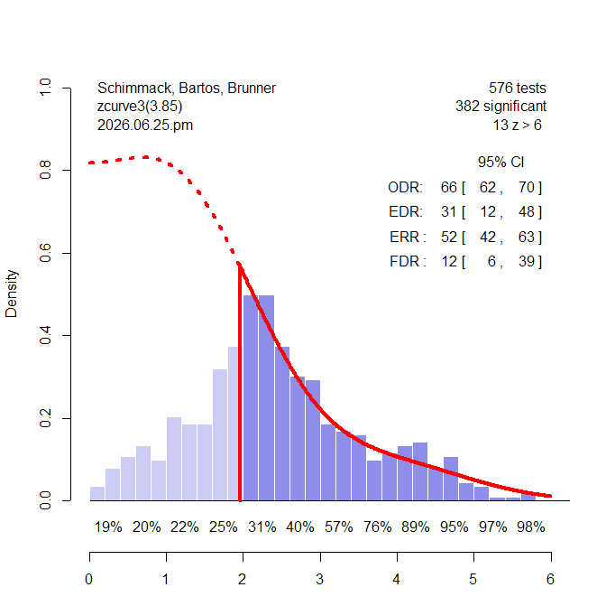
Z-curve fits a finite-mixture model to the distribution of the significant z-values and predicts the distribution of non-significant results from the weights of the mixture components (Figure 2). The z-curve plot shows clear evidence of selection bias. That is there are more observed significant results (66%) than the model predicts (31%). However, the important question is whether the distribution of the non-significant positive z-values matches the predicted distribution shape (the red dotted line in Figure 1).
Visual inspection suggests that this is not the case. There are more observed non-significant results close to the significance criterion than close to zero. In contrast, the predicted pattern shows a flat and then decreasing shape from 0 to 1.65 (values between 1.65 and 1.96 are inconclusive because they are often reported as marginally significant results).
To complement visual inspection with a statistical test, z-curve (version 3.85) compares the distributions while holding the overall density constant (i.e., removing selection bias). A negative difference indicates that there are more z-values close to zero than predicted. A positive difference indicates that there are more z-values close to the significance criterion. A bootstrap confidence interval is used to test for statistical significance.
The median difference was z = .15, 95%CI [ .08, .38]. The mean difference was z = .10, 95%CI = [.05 to .26]. This finding is consistent with the observation that observed z-values close to zero are relatively rare. In short, the observed distribution of the non-significant results is inconsistent with at least one of the assumptions of the step-function model.
The test does not reveal which assumption is violated, and in these data both may be. The depletion of nonsignificant results near zero suggests that selection bias varies within the step, contrary to the assumption that selection is constant within a p-value range. Separately, the near-absence of negative results is hard to reconcile with the model’s estimate of large heterogeneity (tau = .96), which produces a prediction interval for population effect sizes from d = −2.20 to 1.54. A lower bound of −2.20 implies that a substantial share of studies have true effects opposite to the prediction — that mortality primes often produce the reverse of the expected effect. That is implausible; more likely, the negative tail is an artifact of assuming a normal distribution. The shape test cannot identify the true distribution of population effect sizes, but it forces meta-analysts to confront the distribution assumption rather than leave it implicit.
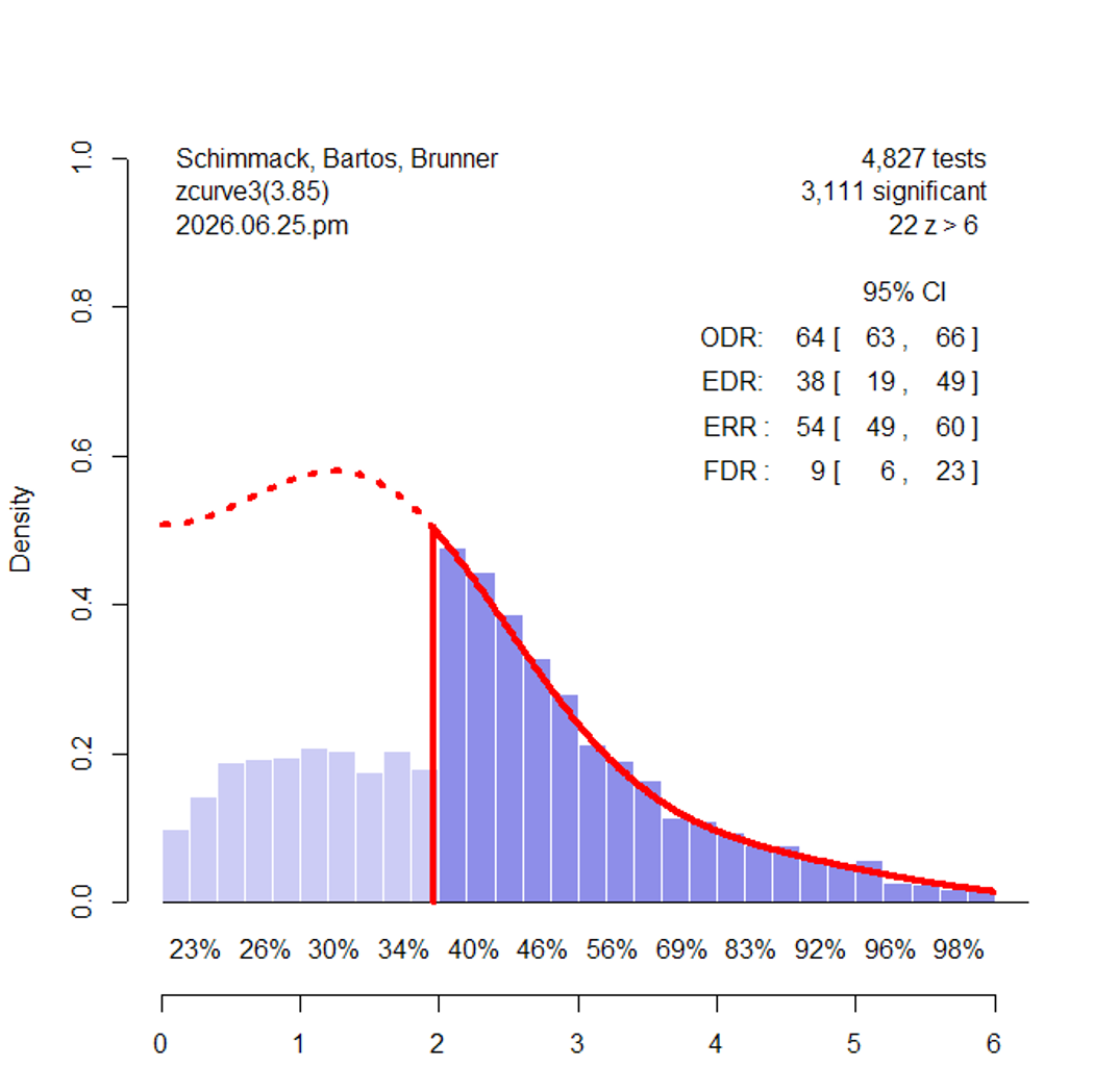
To demonstrate that the shape test works, I used the model weights of the actual data to simulate data without publication bias. I then removed 70% of the non-significant results without changing the distribution of the non-significant results (Figure 2).
Visual inspection shows that the distribution of the non-significant results is more similar to the predicted distribution. The shape test results are consistent with this observation. The median difference is -.05, 95%CI [-.10, .18]. The mean difference is -.04, 95%CI [-.07, .12]. Both confidence intervals include zero.
In sum, step-function models make assumptions about the distribution of population effect sizes and the selection of non-significant results to use observed non-significant results in the estimation of the amount of bias and the average and standard deviation of the population effect sizes. The advantage is that more data reduce random sampling error. The disadvantage is that violations of assumptions can introduce systematic biases. This disadvantage has been neglected in applications of step-function selection models. The ability to test the assumptions has several benefits. First, it draws more attention to the fact that assumptions influence model estimates. Second, shape tests help readers to evaluate the plausibility of the model and to question estimates that are based on data that are inconsistent with assumptions. Third, assumption tests can resolve inconsistencies between estimates obtained with different models. Results based on models that make fewer assumptions or pass assumption tests are more credible than those based on models that do not meet assumptions.
In conclusion, meta-analysts have many tools to analyze their data that often produce inconsistent results. To make sense of these inconsistencies, it is important to understand why they produce inconsistent results. Violated assumptions are one plausible reason and undermine the plausibility of results of these models.
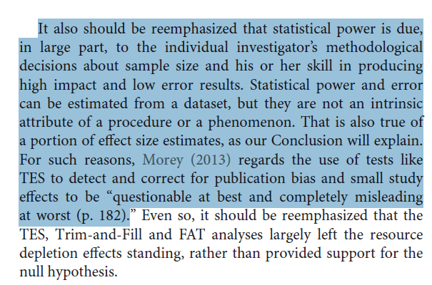
Statistical power is widely known as a tool for planning sample sizes before studies are conducted. Less well known is the use of statistical power after publication to evaluate the credibility of published results in sets of studies, such as meta-analyses.
The basic idea is simple. Statistical power is the probability of obtaining a statistically significant result, typically p < .05. When the null hypothesis is true, this probability equals the alpha criterion, usually 5%. When the null hypothesis is false, power depends on the true population effect size, the sample size, and the significance criterion.
Several publication-bias tests estimate the average power of completed studies and compare it to the actual number of significant results in those studies (Ioannidis & Trikalinos, 2007; Schimmack, 2012). If the observed frequency of significant results is greater than the expected frequency based on average power, this suggests that non-significant results are missing from the published record. This reduces the credibility of the published results. The published literature is less robust than it appears, effect sizes are inflated, and the false-positive risk is higher than the observed success rate suggests.
The negative effects of publication bias on the credibility of published findings are well known and not controversial. Although publication bias is common, there is broad agreement that it is a problem. Publication-bias tests make it possible to detect this problem empirically.
The main challenge for power-based bias tests is estimating the true average power of completed studies. Developing and comparing different estimation methods is an active area of research, but these methods rely on the same basic principle: a set of studies cannot honestly produce substantially more significant results than its average power predicts. With reported success rates above 90% in many psychology journals, power-based tests typically show clear evidence of selection bias.
A few critical articles and blog posts have raised concerns about estimating average true power. However, these criticisms often do not engage with the actual goal of methods that use average power to detect publication bias. For example, McShane et al. acknowledge that average power says “something about replicability if we were able to replicate in the purely hypothetical repeated sampling sense and if we defined success in terms of statistical significance.” McShane objects that this is not useful because new replication studies can differ from original studies. But the purpose of computing average power in meta-analyses of completed studies is not to plan future studies or predict their exact outcomes. The purpose is to examine the credibility of the completed studies.
If a published literature reports 90% significant results but the completed studies had only 20% average power, the published record does not provide credible evidence for the claim, even if it contains hundreds of significant results. Critics of average-statistical power calculations often ignore this important information. Average power is not merely a planning tool. It is also a diagnostic tool for evaluating whether a published body of evidence is too successful to be credible.
I love talking to ChatGPT because it is actually able to process arguments in a rational manner without motivated biases (at least about topics like average power). The document is a transcript of my discussion with ChatGPT about McShane et al.’s article “Average Power: A Cautionary Note” The article has been cited as “evidence” that average power estimates are useless or even fundamentally flawed. As you can see from the discussion that is an overstatement. Like all estimates of unknown population parameters, it is possible that estimates are biased, but the problems are by no means greater than the problems in estimates of other meta-analytic averages. After offering some arguments in favor of using average power estimates, ChatGPT agrees that it can provide useful information to evaluate the presence of publicatoin bias in original studies and to predict the outcome of replication studies and to evaluate discrepancies in success rates between original and replication studies.
Over the past two decades, social psychological research on prejudice has been dominated by the implicit cognition paradigm (Meissner, Grigutsch, Koranyi, Müller, & Rothermund, 2019). This paradigm is based on the assumption that many individuals of the majority group (e.g., White US Americans) have an automatic tendency to discriminate against members of a stigmatized minority group (e.g., African Americans). It is assumed that this tendency is difficult to control because many people are unaware of their prejudices.
The implicit cognition paradigm also assumes that biases vary across individuals of the majority group. The most widely used measure of individual differences in implicit biases is the race Implicit Association Test (rIAT; Greenwald, McGhee, & Schwartz, 1998). Like any other measure of individual differences, the race IAT has to meet psychometric criteria to be a useful measure of implicit bias. Unfortunately, the race IAT has been used in hundreds of studies before its psychometric properties were properly evaluated in a program of validation research (Schimmack, 2021a, 2021b).
Meta-analytic reviews of the literature suggest that the race IAT is not as useful for the study of prejudice as it was promised to be (Greenwald et al., 1998). For example, Meissner et al. (2019) concluded that “the predictive value for behavioral criteria is weak and their incremental validity over and above self-report measures is negligible” (p. 1).
In response to criticism of the race IAT, Greenwald, Banaji, and Nosek (2015) argued that “statistically small effects of the implicit association test can have societally large effects” (p. 553). At the same time, Greenwald (1975) warned psychologists that they may be prejudiced against the null-hypothesis. To avoid this bias, he proposed that researchers should define a priori a range of effect sizes that are close enough to zero to decide in favor of the null-hypothesis. Unfortunately, Greenwald did not follow his own advice and a clear criterion for a small, but practically significant amount of predictive validity is lacking. This is a problem because estimates have decreased over time from r = .39 (McConnell & Leibold, 2001), to r = .24 in 2009 ( Greenwald, Poehlman, Uhlmann, and Banaji, 2009), to r = .148 in 2013 (Oswald, Mitchell, Blanton, Jaccard, & Tetlock (2013), and r = .097 in 2019 (Greenwald & Lai, 2020; Kurdi et al., 2019). Without a clear criterion value, it is not clear how this new estimate of predictive validity should be interpreted. Does it still provide evidence for a small, but practically significant effect, or does it provide evidence for the null-hypothesis (Greenwald, 1975)?
Measures are not Causes
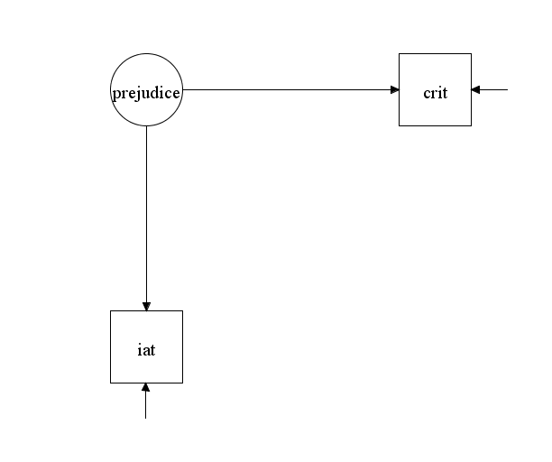
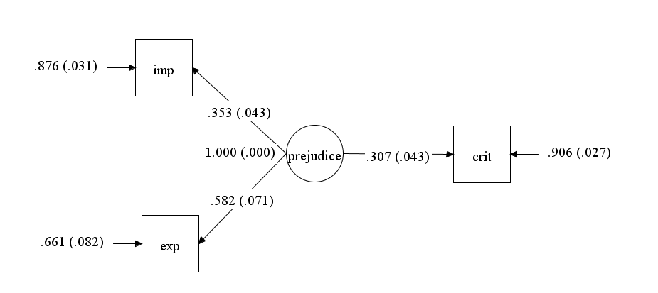
To justify the interpretation of a correlation of r = .1 as small but important, it is important to revisit Greenwald et al.’s (2015) arguments for this claim. Greenwald et al. (2015) interpret this correlation as evidence for an effect of the race IAT on behavior. For example, they write “small effects can produce substantial discriminatory impact also by cumulating over repeated occurrences to the same person” (p. 558). The problem with this causal interpretation of a correlation between two measures is that scores on the race IAT have no influence on individuals’ behavior. This simple fact is illustrated in Figure 1. Figure 1 is a causal model that assumes the race IAT reflects valid variance in prejudice and prejudice influences actual behaviors (e.g., not voting for a Black political candidate). The model makes it clear that the correlation between scores on the race IAT (i.e., the iat box) and scores on a behavioral measures (i.e., the crit box) do not have a causal link (i.e., no path leads from the iat box to the crit box). Rather, the two measured variables are correlated because they both reflect the effect of a third variable. That is, prejudice influences race IAT scores and prejudice influences the variance in the criterion variable.
There is general consensus among social scientists that prejudice is a problem and that individual differences in prejudice have important consequences for individuals and society. The effect size of prejudice on a single behavior has not been clearly examined, but to the extent that race IAT scores are not perfectly valid measures of prejudice, the simple correlation of r = .1 is a lower limit of the effect size. Schimmack (2021) estimated that no more than 20% of the variance in race IAT scores is valid variance. With this validity coefficient, a correlation of r = .1 implies an effect of prejudice on actual behaviors of .1 / sqrt(.2) = .22.
Greenwald et al. (2015) correctly point out that effect sizes of this magnitude, r ~ .2, can have practical, real-world implications. The real question, however, is whether predictive validity of .1 justifies the use of the race IAT as a measure of prejudice. This question has to be evaluated in a comparison of predictive validity for the race IAT with other measures of prejudice. Thus, the real question is whether the race IAT has sufficient incremental predictive validity over other measures of prejudice. However, this question has been largely ignored in the debate about the utility of the race IAT (Greenwald & Lai, 2020; Greenwald et al., 2015; Oswald et al., 2013).
Kurdi et al. (2019) discuss incremental predictive validity, but this discussion is not limited to the race IAT and makes the mistake to correct for random measurement error. As a result, the incremental predictive validity for IATs of b = .14 is a hypothetical estimate for IATs that are perfectly reliable. However, it is well-known that IATs are far from perfectly reliable. Thus, this estimate overestimates the incremental predictive validity. Using Kurdi et al.’s data and limiting the analysis to studies with the race IAT, I estimated incremental predictive validity to be b = .08, 95%CI = .04 to .12. It is difficult to argue that this a practically significant amount of incremental predictive validity. At the very least, it does not justify the reliance on the race IAT as the only measure of prejudice or the claim that the race IAT is a superior measure of prejudice (Greenwald et al., 2009).
The meta-analytic estimate of b = .1 has to be interpreted in the context of evidence of substantial heterogeneity across studies (Kurdi et al., 2019). Kurdi et al. (2019) suggest that “it may be more appropriate to ask under what conditions the two [race IAT scores and criterion variables] are more or less highly correlated” (p. 575). However, little progress has been made in uncovering moderators of predictive validity. One possible explanation for this is that previous meta-analysis may have overlooked one important source of variation in effect sizes, namely publication bias. Traditional meta-analyses may be unable to reveal publication bias because they include many articles and outcome measures that did not focus on predictive validity. For example, Kurdi’s meta-analysis included a study by Luo, Li, Ma, Zhang, Rao, and Han (2015). The main focus of this study was to examine the potential moderating influence of oxytocin on neurological responses to pain expressions of Asian and White faces. Like many neurological studies, the sample size was small (N = 32), but the study reported 16 brain measures. For the meta-analysis, correlations were computed across N = 16 participants separately for two experimental conditions. Thus, this study provided as many effect sizes as it had participants. Evidently, power to obtain a significant result with N = 16 and r = .1 is extremely low, and adding these 32 effect sizes to the meta-analysis merely introduced noise. This may undermine the validity of meta-analytic results ((Sharpe, 1997). To address this concern, I conducted a new meta-analysis that differs from the traditional meta-analyses. Rather than coding as many effects from as many studies as possible, I only include focal hypothesis tests from studies that aimed to investigate predictive validity. I call this a focused meta-analysis.
Focused Meta-Analysis of Predictive Validity
Coding of Studies
I relied on Kurdi et al.’s meta-analysis to find articles. I selected only published articles that used the race IAT (k = 96). The main purpose of including unpublished studies is often to correct for publication bias (Kurdi et al., 2019). However, it is unlikely that only 14 (8%) studies that were conducted remained unpublished. Thus, the unpublished studies are not representative and may distort effect size estimates.
Coding of articles in terms of outcome measures that reflect discrimination yielded 60 studies in 45 articles. I examined whether this selection of studies influenced the results by limiting a meta-analysis with Kurdi et al.’s coding of studies to these 60 articles. The weighted average effect size was larger than the reported effect size, a = .167, se = .022, 95%CI = .121 to .212. Thus, Kurdi et al.’s inclusion of a wide range of studies with questionable criterion variables diluted the effect size estimate. However, there remained substantial variability around this effect size estimate using Kurdi et al.’s data, I2 = 55.43%.
Results
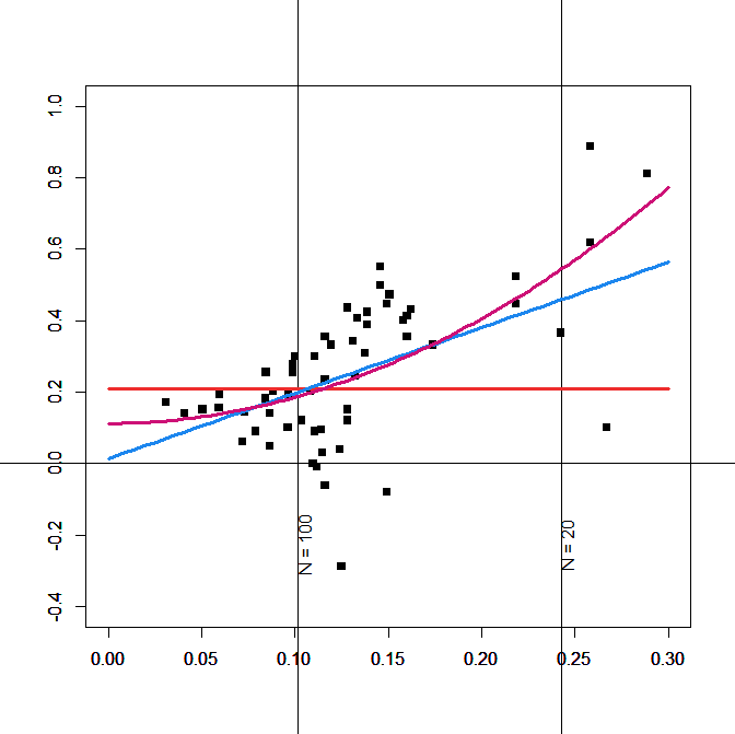
The focused coding produced one effect-size per study. It is therefore not necessary to model a nested structure of effect sizes and I used the widely used metafor package to analyze the data (Viechtbauer, 2010). The intercept-only model produced a similar estimate to the results for Kurdi et al.’s coding scheme, a = .201, se = .020, 95%CI = .171 to .249. Thus, focal coding does seem to produce the same effect size estimate as traditional coding. There was also a similar amount of heterogeneity in the effect sizes, I2 = 50.80%.
However, results for publication bias differed. Whereas Kurdi et al.’s coding shows no evidence of publication bias, focused coding produced a significant relationship emerged, b = 1.83, se = .41, z = 4.54, 95%CI = 1.03 to 2.64. The intercept was no longer significant, a = .014, se = .0462, z = 0.31, 95%CI = -.077 to 95%CI = .105. This would imply that the race IAT has no incremental predictive validity. Adding sampling error as a predictor reduced heterogeneity from I2 = 50.80% to 37.71%. Thus, some portion of the heterogeneity is explained by publication bias.
Stanley (2017) recommends to accept the null-hypothesis when the intercept in the previous model is not significant. However, a better criterion is to compare this model to other models. The most widely used alternative model regresses effect sizes on the squared sampling error (Stanley, 2017). This model explained more of the heterogeneity in effect sizes as reflected in a reduction of unexplained heterogeneity from 50.80% to 23.86%. The intercept for this model was significant, a = .113, se = .0232, z = 4.86, 95%CI = .067 to .158.
Figure 2 shows the effect sizes as a function of sampling error and the regression lines for the three models.
Inspection of Figure 1 provides further evidence that the squared-SE model. The red line (squared sampling error) fits the data better than the blue line (sampling error) model. In particular for large samples, PET underestimates effect sizes.
The significant relationship between sample size (sampling error) and effect sizes implies that large effects in small studies cannot be interpreted at face value. For example, the most highly cited study of predictive validity had only a sample size of N = 42 participants (McConnell & Leibold, 2001). The squared-sampling-error model predicts an effect size estimate of r = .30, which is close to the observed correlation of r = .39 in that study.
In sum, a focal meta-analysis replicates Kurdi et al.’s (2019) main finding that the average predictive validity of the race IAT is small, r ~ .1. However, the focal meta-analysis also produced a new finding. Whereas the initial meta-analysis suggested that effect sizes are highly variable, the new meta-analysis suggests that a large portion of this variability is explained by publication bias.
Moderator Analysis
I explored several potential moderator variables, namely (a) number of citations, (b) year of publication, (c) whether IAT effects were direct or moderator effects, (d) whether the correlation coefficient was reported or computed based on test statistics, and (e) whether the criterion was an actual behavior or an attitude measure. The only statistically significant result was a weaker correlation in studies that predicted a moderating effect of the race IAT, b = -.11, se = .05, z = 2.28, p = .032. However, the effect would not be significant after correction for multiple comparison and heterogeneity remained virtually unchanged, I2 = 27.15%.
During the coding of the studies, the article “Ironic effects of racial bias during interracial interactions” stood out because it reported a counter-intuitive result. in this study, Black confederates rated White participants with higher (pro-White) race IAT scores as friendlier. However, other studies find the opposite effect (e.g., McConnell & Leibold, 2001). If the ironic result was reported because it was statistically significant, it would be a selection effect that is not captured by the regression models and it would produce unexplained heterogeneity. I therefore also tested a model that excluded all negative effect. As bias is introduced by this selection, the model is not a test of publication bias, but it may be better able to correct for publication bias. The effect size estimate was very similar, a = .133, se = .017, 95%CI = .010 to .166. However, heterogeneity was reduced to 0%, suggesting that selection for significance fully explains heterogeneity in effect sizes.
In conclusion, moderator analysis did not find any meaningful moderators and heterogeneity was fully explained by publication bias, including publishing counterintuitive findings that suggest less discrimination by individuals with more prejudice. The finding that publication bias explains most of the variance is extremely important because Kurdi et al. (2019) suggested that heterogeneity is large and meaningful, which would suggest that higher predictive validity could be found in future studies. In contrast, the current results suggest that correlations greater than .2 in previous studies were largely due to selection for significance with small samples, which also explains unrealistically high correlations in neuroscience studies with the race IAT (cf. Schimmack, 2021b).
Predictive Validity of Self-Ratings
The predictive validity of self-ratings is important for several reasons. First, it provides a comparison standard for the predictive validity of the race IAT. For example, Greenwald et al. (2009) emphasized that predictive validity for the race IAT was higher than for self-reports. However, Kurdi et al.’s (2019) meta-analysis found the opposite. Another reason to examine the predictive validity of explicit measures is that implicit and explicit measures of racial attitudes are correlated with each other. Thus, it is important to establish the predictive validity of self-ratings to estimate the incremental predictive validity of the race IAT.
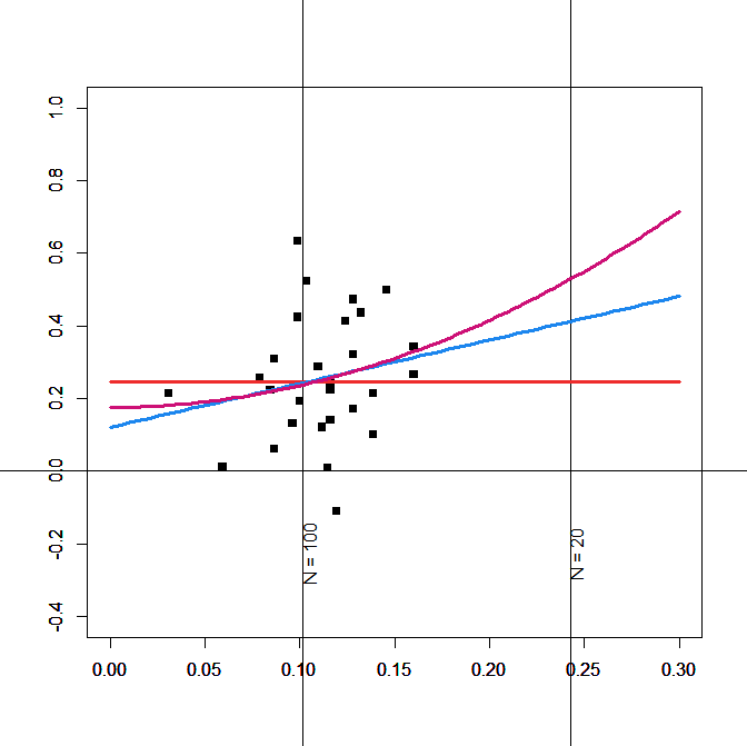
Figure 2 shows the results. The sampling-error model shows a non-zero effect size, but sampling error is large, and the confidence interval includes zero, a = .121, se = .117, 95%CI = -.107 to .350. Effect sizes are also extremely heterogeneous, I2 = 62.37%. The intercept for the squared-sampling-error model is significant, a = .176, se = .071, 95%CI = .036 to .316, but the model does not explain more of the heterogeneity in effect sizes than the squared-sampling-error model, I2 = 63.33%. To remain comparability, I use the squared-sampling error estimate. This confirms Kurdi et al.’s finding that self-ratings have slightly higher predictive validity, but the confidence intervals overlap. For any practical purposes, predictive validity of the race IAT and self-reports is similar. Repeating the moderator analyses that were conducted with the race IAT revealed no notable moderators.
Implicit-Explicit Correlations
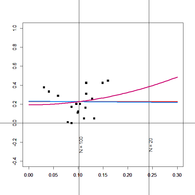
Only 21 of the 60 studies reported information about the correlation between the race IAT and self-report measures. There was no indication of publication bias, and the effect size estimates of the three models converge on an estimate of r ~ .2 (Figure 3). Fortunately, this result can be compared with estimates from large internet studies (Axt, 2017) and a meta-analysis of implicit-explicit correlations (Hofmann et al., 2005). These estimates are a bit higher, r ~ .25. Thus, using an estimate of r = .2 is conservative for a test of the incremental predictive validity of the race IAT.
Incremental Predictive Validity
It is straightforward to estimate the incremental predictive validity of the race IAT and self-reports on the basis of the correlations between race IAT, self-ratings, and criterion variables. However, it is a bit more difficult to provide confidence intervals around these estimates. I used a simulated dataset with missing values to reproduce the correlations and sampling error of the meta-analysis. I then regressed, the criterion on the implicit and explicit variable. The incremental predictive validity for the race IAT was b = .07, se = .02, 95%CI = .03 to .12. This finding implies that the race IAT on average explains less than 1% unique variance in prejudice behavior. The incremental predictive validity of the explicit measure was b = .165, se = .03, 95%CI = .11 to .23. This finding suggests that explicit measures explain between 1 and 4 percent of the variance in prejudice behaviors.
Assuming that there is no shared method variance between implicit and explicit measures and criterion variables and that implicit and explicit measures reflect a common construct, prejudice, it is possible to fit a latent variable model to the correlations among the three indicators of prejudice (Schimmack, 2021). Figure 4 shows the model and the parameter estimates.
According to this model, prejudice has a moderate effect on behavior, b = .307, se = .043. This is consistent with general findings about effects of personality traits on behavior (Epstein, 1973; Funder & Ozer, 1983). The loading of the explicit variable on the prejudice factor implies that .582^2 = 34% of the variance in self-ratings of prejudice is valid variance. The loading of the implicit variable on the prejudice factor implies that .353^2 = 12% of the variance in race IAT scores is valid variance. Notably, similar estimates were obtained with structural equation models of data that are not included in this meta-analysis (Schimmack, 2021). Using data from Cunningham et al., (2001) I estimated .43^2 = 18% valid variance. Using Bar-Anan and Vianello (2018), I estimated .44^2 = 19% valid variance. Using data from Axt, I found .44^2 = 19% valid variance, but 8% of the variance could be attributed to group differences between African American and White participants. Thus, the present meta-analytic results are consistent with the conclusion that no more than 20% of the variance in race IAT scores reflects actual prejudice that can influence behavior.
In sum, incremental predictive validity of the race IAT is low for two reasons. First, prejudice has only modest effects on actual behavior in a specific situation. Second, only a small portion of the variance in race IAT scores is valid.
Discussion
In the 1990s, social psychologists embraced the idea that behavior is often influenced by processes that occur without conscious awareness. This assumption triggered the implicit revolution (Greenwald & Banaji, 2017). The implicit paradigm provided a simple explanation for low correlations between self-ratings of prejudice and implicit measures of prejudice, r ~ .2. Accordingly, many people are not aware how prejudice their unconscious is. The Implicit Association Test seemed to support this view because participants showed more prejudice on the IAT than on self-report measures. First studies of predictive validity also seemed to support this new model of prejudice (McConnell & Leibold, 2001), and the first meta-analysis suggested that implicit bias has a stronger influence on behavior than self-reported attitudes (Greenwald, Poehlman, Uhlmann, & Banaji, 2009, p. 17).
However, the following decade produced many findings that require a reevaluation of the evidence. Greenwald et al. (2009) published the largest test (N = 1057) of predictive validity. This study examined the ability of the race IAT to predict racial bias in the 2008 US presidential election. Although the race IAT was correlated with voting for McCain versus Obama, incremental predictive validity was close to zero and no longer significant when explicit measures were included in the regression model. Then subsequent meta-analyses produced lower estimates of predictive validity and it is no longer clear that predictive validity, especially incremental predictive validity, is high enough to reject the null-hypothesis. Although incremental predictive validity may vary across conditions, no conditions have been identified that show practically significant incremental predictive validity. Unfortunately, IAT proponents continue to make misleading statements based on single studies with small samples. For example, Kurdi et al. claimed that “effect sizes tend to be relatively large in studies on physician–patient interactions” (p. 583). However, this claim was based on a study with just 15 physicians, which makes it impossible to obtain precise effect size estimates about implicit bias effects for physicians.
Beyond Nil-Hypothesis Testing
Just like psychology in general, meta-analyses also suffer from the confusion of nil-hypothesis testing and null-hypothesis testing. The nil-hypothesis is the hypothesis that an effect size is exactly zero. Many methodologists have pointed out that it is rather silly to take the nil-hypothesis at face value because the true effect size is rarely zero (Cohen, 1994). The more important question is whether an effect size is sufficiently different from zero to be theoretically and practically meaningful. As pointed out by Greenwald (1975), effect size estimation has to be complemented with theoretical predictions about effect sizes. However, research on predictive validity of the race IAT lacks clear criteria to evaluate effect size estimates.
As noted in the introduction, there is agreement about the practical importance of statistically small effects for the prediction of discrimination and other prejudiced behaviors. The contentious question is whether the race IAT is a useful measure of dispositions to act prejudiced. Viewed from this perspective, focus on the race IAT is myopic. The real challenge is to develop and validate measures of prejudice. IAT proponents have often dismissed self-reports as invalid, but the actual evidence shows that self-reports have some validity that is at least equal to the validity of the race IAT. Moreover, even distinct self-report measures like the feeling thermometer and the symbolic racism have incremental predictive validity. Thus, prejudice researchers should use a multi-method approach. At present it is not clear that the race IAT can improve the measurement of prejudice (Greenwald et al., 2009; Schimmack, 2021a).
Methodological Implications
This article introduced a new type of meta-analysis. Rather than trying to find as many vaguely related studies and to code as many outcomes as possible, focused meta-analysis is limited to the main test of the key hypothesis. This approach has several advantages. First, the classic approach creates a large amount of heterogeneity that is unique to a few studies. This noise makes it harder to find real moderators. Second, the inclusion of vaguely related studies may dilute effect sizes. Third, the inclusion of non-focal studies may mask evidence of publication bias that is virtually present in all literatures. Finally, focal meta-analysis are much easier to do and can produce results much faster than the laborious meta-analyses that psychologists are used to. Even when classic meta-analysis exist, they often ignore publication bias. Thus, an important task for the future is to complement existing meta-analysis with focal meta-analysis to ensure that published effect sizes estimates are not diluted by irrelevant studies and not inflated by publication bias.
Prejudice Interventions
Enthusiasm about implicit biases has led to interventions that aim to reduce implicit biases. This focus on implicit biases in the real world needs to be reevaluated. First, there is no evidence that prejudice typically operates outside of awareness (Schimmack, 2021a). Second, individual differences in prejudice have only a modest impact on actual behaviors and are difficult to change. Not surprisingly, interventions that focus on implicit bias are not very infective. Rather than focusing on changing individuals’ dispositions, interventions may be more effective by changing situations. In this regard, the focus on internal factors is rather different from the general focus in social psychology on situational factors (Funder & Ozer, 1983). In recent years, it has become apparent that prejudice is often systemic. For example, police training may have a much stronger influence on racial disparities in fatal use of force than individual differences in prejudice of individual officers (Andersen, Di Nota, Boychuk, Schimmack, & Collins, 2021).
Conclusion
The present meta-analysis of the race IAT provides further support for Meissner et al.’s (2019) conclusion that IATs “predictive value for behavioral criteria is weak and their incremental validity over and above self-report measures is negligible” (p. 1). The present meta-analysis provides a quantitative estimate of b = .07. Although researchers can disagree about the importance of small effect sizes, I agree with Meissner that the gains from adding a race IAT to the measurement of prejudice is negligible. Rather than looking for specific contexts in which the race IAT has higher predictive validity, researchers should use a multi-method approach to measure prejudice. The race IAT may be included to further explore its validity, but there is no reason to rely on the race IAT as the single most important measure of individual differences in prejudice.
References
Funder, D.C., & Ozer, D.J. (1983). Behavior as a function of the situation. Journal of Personality and Social Psychology, 44, 107–112.
Kurdi, B., Seitchik, A. E., Axt, J. R., Carroll, T. J., Karapetyan, A., Kaushik, N., et al. (2019). Relationship between the implicit association test and intergroup behavior: a meta-analysis. American Psychologist. 74, 569–586. doi: 10.1037/amp0000364
Viechtbauer, W. (2010). Conducting meta-analyses in R with the metafor package. Journal of Statistical Software, 36(3), 1–48. https://www.jstatsoft.org/v036/i03.
After I posted this post, I learned about a published meta-analysis and new studies of incidental anchoring by David Shanks and colleagues that came to the same conclusion (Shanks et al., 2020).
Introduction
“The most expensive car in the world costs $5 million. How much does a new BMW 530i cost?”
According to anchoring theory, information about the most expensive car can lead to higher estimates for the cost of a BMW. Anchoring effects have been demonstrated in many credible studies since the 1970s (Kahneman & Tversky, 1973).
A more controversial claim is that anchoring effects even occur when the numbers are unrelated to the question and presented incidentally (Criticher & Gilovich, 2008). In one study, participants saw a picture of a football player and were asked to guess how likely it is that the player will sack the football player in the next game. The player’s number on jersey was manipulated to be 54 or 94. The study produced a statistically significant result suggesting that a higher number makes people give higher likelihood judgments. This study started a small literature on incidental anchoring effects. A variation on this them are studies that presented numbers so briefly on a computer screen that most participants did not actually see the numbers. This is called subliminal priming. Allegedly, subliminal priming also produced anchoring effects (Mussweiler & Englich (2005).
Since 2011, many psychologists are skeptical whether statistically significant results in published articles can be trusted. The reason is that researchers only published results that supported their theoretical claims even when the claims were outlandish. For example, significant results also suggested that extraverts can foresee where pornographic images are displayed on a computer screen even before the computer randomly selected the location (Bem, 2011). No psychologist, except Bem, believes these findings. More problematic is that many other findings are equally incredible. A replication project found that only 25% of results in social psychology could be replicated (Open Science Collaboration, 2005). So, the question is whether incidental and subliminal anchoring are more like classic anchoring or more like extrasensory perception.
There are two ways to assess the credibility of published results when publication bias is present. One approach is to conduct credible replication studies that are published independent of the outcome of a study. The other approach is to conduct a meta-analysis of the published literature that corrects for publication bias. A recent article used both methods to examine whether incidental anchoring is a credible effect (Kvarven et al., 2020). In this article, the two approaches produced inconsistent results. The replication study produced a non-significant result with a tiny effect size, d = .04 (Klein et al., 2014). However, even with bias-correction, the meta-analysis suggested a significant, small to moderate effect size, d = .40.
Results
The data for the meta-analysis were obtained from an unpublished thesis (Henriksson, 2015). I suspected that the meta-analysis might have coded some studies incorrectly. Therefore, I conducted a new meta-analysis, using the same studies and one new study. The main difference between the two meta-analysis is that I coded studies based on the focal hypothesis test that was used to claim evidence for incidental anchoring. The p-values were then transformed into fisher-z transformed correlations and and sampling error, 1/sqrt(N – 3), based on the sample sizes of the studies.
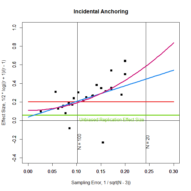
Whereas the old meta-analysis suggested that there is no publication bias, the new meta-analysis showed a clear relationship between sampling error and effect sizes, b = 1.68, se = .56, z = 2.99, p = .003. Correcting for publication bias produced a non-significant intercept, b = .039, se = .058, z = 0.672, p = .502, suggesting that the real effect size is close to zero.
Figure 1 shows the regression line for this model in blue and the results from the replication study in green. We see that the blue and green lines intersect when sampling error is close to zero. As sampling error increases because sample sizes are smaller, the blue and green line diverge more and more. This shows that effect sizes in small samples are inflated by selection for significance.
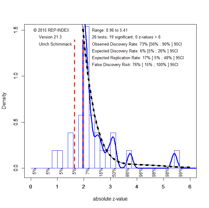
However, there is some statistically significant variability in the effect sizes, I2 = 36.60%, p = .035. To further examine this heterogeneity, I conducted a z-curve analysis (Bartos & Schimmack, 2021; Brunner & Schimmack, 2020). A z-curve analysis converts p-values into z-statistics. The histogram of these z-statistics shows publication bias, when z-statistics cluster just above the significance criterion, z = 1.96.
Figure 2 shows a big pile of just significant results. As a result, the z-curve model predicts a large number of non-significant results that are absent. While the published articles have a 73% success rate, the observed discovery rate, the model estimates that the expected discovery rate is only 6%. That is, for every 100 tests of incidental anchoring, only 6 studies are expected to produce a significant result. To put this estimate in context, with alpha = .05, 5 studies are expected to be significant based on chance alone. The 95% confidence interval around this estimate includes 5% and is limited at 26% at the upper end. Thus, researchers who reported significant results did so based on studies with very low power and they needed luck or questionable research practices to get significant results.
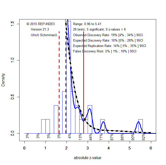
A low discovery rate implies a high false positive risk. With an expected discovery rate of 6%, the false discovery risk is 76%. This is unacceptable. To reduce the false discovery risk, it is possible to lower the alpha criterion for significance. In this case, lowering alpha to .005 produces a false discovery risk of 5%. This leaves 5 studies that are significant.
One notable study with strong evidence, z = 3.70, examined anchoring effects for actual car sales. The data came from an actual auction of classic cars. The incidental anchors were the prices of the previous bid for a different vintage car. Based on sales data of 1,477 cars, the authors found a significant effect, b = .15, se = .04 that translates into a standardized effect size of d = .2 (fz = .087). Thus, while this study provides some evidence for incidental anchoring effects in one context, the effect size estimate is also consistent with the broader meta-analysis that effect sizes of incidental anchors are fairly small. Moreover, the incidental anchor in this study is still in the focus of attention and in some way related to the actual bid. Thus, weaker effects can be expected for anchors that are not related to the question at all (a player’s number) or anchors presented outside of awareness.
Conclusion
There is clear evidence that evidence for incidental anchoring cannot be trusted at face value. Consistent with research practices in general, studies on incidental and subliminal anchoring suffer from publication bias that undermines the credibility of the published results. Unbiased replication studies and meta-analysis suggest that incidental anchoring effects are either very small or zero. Thus, there exists currently no empirical support for the notion that irrelevant numeric information can bias numeric judgments. More research on anchoring effects that corrects for publication bias is needed.
Social psychologists have failed to clean up their act and their literature. Here I show unusually high effect sizes in non-retracted articles by Sanna, who retracted several articles. I point out that non-retraction does not equal credibility and I show that co-authors like Norbert Schwarz lack any motivation to correct the published record. The inability of social psychologists to acknowledge and correct their mistakes renders social psychology a para-science that lacks credibility. Even meta-analyses cannot be trusted because they do not correct properly for the use of questionable research practices.
Introduction
When I grew up, a popular German Schlager was the song “Aber bitte mit Sahne.” The song is about Germans love of deserts with whipped cream. So, when I saw articles by Sanna, I had to think about whipped cream, which is delicious. Unfortunately, articles by Sanna are the exact opposite. In the early 2010s, it became apparent that Sanna had fabricated data. However, unlike the thorough investigation of a similar case in the Netherlands, the extent of Sanna’s fraud remains unclear (Retraction Watch, 2012). The latest count of Sanna’s retracted articles was 8 (Retraction Watch, 2013).
WebOfScience shows 5 retraction notices for 67 articles, which means 62 articles have not been retracted. The question is whether these article can be trusted to provide valid scientific information? The answer to this question matters because Sanna’s articles are still being cited at a rate of over 100 citations per year.
Meta-Analysis of Ease of Retrieval
The data are also being used in meta-analyses (Weingarten & Hutchinson, 2018). Fraudulent data are particularly problematic for meta-analysis because fraud can produce large effect size estimates that may inflate effect size estimates. Here I report the results of my own investigation that focusses on the ease-of-retrieval paradigm that was developed by Norbert Schwarz and colleagues (Schwarz et al., 1991).
The meta-analysis included 7 studies from 6 articles. Two studies produced independent effect size estimates for 2 conditions for a total of 9 effect sizes.
Sanna, L. J., Schwarz, N., & Small, E. M. (2002). Accessibility experiences and the hindsight bias: I knew it all along versus it could never have happened. Memory & Cognition, 30(8), 1288–1296. https://doi.org/10.3758/BF03213410 [Study 1a, 1b]
Sanna, L. J., Schwarz, N., & Stocker, S. L. (2002). When debiasing backfires: Accessible content and accessibility experiences in debiasing hindsight. Journal of Experimental Psychology: Learning, Memory, and Cognition, 28(3), 497–502. https://doi.org/10.1037/0278-7393.28.3.497 [Study 1 & 2]
Sanna, L. J., & Schwarz, N. (2003). Debiasing the hindsight bias: The role of accessibility experiences and (mis)attributions. Journal of Experimental Social Psychology, 39(3), 287–295. https://doi.org/10.1016/S0022-1031(02)00528-0 [Study 1]
Sanna, L. J., Chang, E. C., & Carter, S. E. (2004). All Our Troubles Seem So Far Away: Temporal Pattern to Accessible Alternatives and Retrospective Team Appraisals. Personality and Social Psychology Bulletin, 30(10), 1359–1371. https://doi.org/10.1177/0146167204263784 [Study 3a]
Sanna, L. J., Parks, C. D., Chang, E. C., & Carter, S. E. (2005). The Hourglass Is Half Full or Half Empty: Temporal Framing and the Group Planning Fallacy. Group Dynamics: Theory, Research, and Practice, 9(3), 173–188. https://doi.org/10.1037/1089-2699.9.3.173 [Study 3a, 3b]
Carter, S. E., & Sanna, L. J. (2008). It’s not just what you say but when you say it: Self-presentation and temporal construal. Journal of Experimental Social Psychology, 44(5), 1339–1345. https://doi.org/10.1016/j.jesp.2008.03.017 [Study 2]
When I examined Sanna’s results, I found that all 9 of these 9 effect sizes were extremely large with effect size estimates being larger than one standard deviation. A logistic regression analysis that predicted authorship (With Sanna vs. Without Sanna) showed that the large effect sizes in Sanna’s articles were unlikely to be due to sampling error alone, b = 4.6, se = 1.1, t(184) = 4.1, p = .00004 (1 / 24,642).
These results show that Sanna’s effect sizes are not typical for the ease-of-retrieval literature. As one of his retracted articles used the ease-of retrieval paradigm, it is possible that these articles are equally untrustworthy. As many other studies have investigated ease-of-retrieval effects, it seems prudent to exclude articles by Sanna from future meta-analysis.
These articles should also not be cited as evidence for specific claims about ease-of-retrieval effects for the specific conditions that were used in these studies. As the meta-analysis shows, there have been no credible replications of these studies and it remains unknown how much ease of retrieval may play a role under the specified conditions in Sanna’s articles.
Discussion
The blog post is also a warning for young scientists and students of social psychology that they cannot trust researchers who became famous with the help of questionable research practices that produced too many significant results. As the reference list shows, several articles by Sanna were co-authored by Norbert Schwarz, the inventor of the ease-of-retrieval paradigm. It is most likely that he was unaware of Sanna’s fraudulent practices. However, he seemed to lack any concerns that the results might be too good to be true. After all, he encountered replicaiton failures in his own lab.
“of course, we had studies that remained unpublished. Early on we experimented with different manipulations. The main lesson was: if you make the task too blatantly difficult, people correctly conclude the task is too difficult and draw no inference about themselves. We also had a couple of studies with unexpected gender differences” (Schwarz, email communication, 5/18,21).
So, why was he not suspicious when Sanna only produced successful results? I was wondering whether Schwarz had some doubts about these studies with the help of hindsight bias. After all, a decade or more later, we know that he committed fraud for some articles on this topic, we know about replication failures in larger samples (Yeager et al., 2019), and we know that the true effect sizes are much smaller than Sanna’s reported effect sizes (Weingarten & Hutchinson, 2018).
Hi Norbert, thank you for your response. I am doing my own meta-analysis of the literature as I have some issues with the published one by Evan. More about that later. For now, I have a question about some articles that I came across, specifically Sanna, Schwarz, and Small (2002). The results in this study are very strong (d ~ 1). Do you think a replication study powered for 95% power with d = .4 (based on meta-analysis) would produce a significant result? Or do you have concerns about this particular paradigm and do not predict a replication failure? Best, Uli (email
His response shows that he is unwilling or unable to even consider the possibility that Sanna used fraud to produce the results in this article that he co-authored.
Uli, that paper has 2 experiments, one with a few vs many manipulation and one with a facial manipulation. I have no reason to assume that the patterns won’t replicate. They are consistent with numerous earlier few vs many studies and other facial manipulation studies (introduced by Stepper & Strack, JPSP, 1993). The effect sizes always depend on idiosyncracies of topic, population, and context, which influence accessible content and accessibility experience. The theory does not make point predictions and the belief that effect sizes should be identical across decades and populations is silly — we’re dealing with judgments based on accessible content, not with immutable objects.
This response is symptomatic of social psychologists response to decades of research that has produced questionable results that often fail to replicate (see Schimmack, 2020, for a review). Even when there is clear evidence of questionable practices, journals are reluctant to retract articles that make false claims based on invalid data (Kitayama, 2020). And social psychologist Daryl Bem wants rather be remembered as loony para-psychologists than as real scientists (Bem, 2021).
The problem with these social psychologists is not that they made mistakes in the way they conducted their studies. The problem is their inability to acknowledge and correct their mistakes. While they are clinging to their CVs and H-Indices to protect their self-esteem, they are further eroding trust in psychology as a science and force junior scientists who want to improve things out of academia (Hilgard, 2021). After all, the key feature of science that distinguishes it from ideologies is the ability to correct itself. A science that shows no signs of self-correction is a para-science and not a real science. Thus, social psychology is currently para-science (i.e., “Parascience is a broad category of academic disciplines, that are outside the scope of scientific study, Wikipedia).
The only hope for social psychology is that young researchers are unwilling to play by the old rules and start a credibility revolution. However, the incentives still favor conformists who suck up to the old guard. Thus, it is unclear if social psychology will ever become a real science. A first sign of improvement would be to retract articles that make false claims based on results that were produced with questionable research practices. Instead, social psychologists continue to write review articles that ignore the replication crisis (Schwarz & Strack, 2016) as if repression can bend reality.
Citation and link to the actual article: Bartoš, F. & Schimmack, U. (2022). Z‑curve 2.0: Estimating replication rates and discovery rates. Meta‑Psychology, Volume 6, Issue 4, Article MP.2021.2720. Published September 1, 2022. DOI:https://doi.org/10.15626/MP.2021.2720
Update July 14, 2021
After trying several traditional journals that are falsely considered to be prestigious because they have high impact factors, we are proud to announce that our manuscript “Z-curve 2.0: : Estimating Replication Rates and Discovery Rates” has been accepted for publication in Meta-Psychology. We received the most critical and constructive comments of our manuscript during the review process at Meta-Psychology and are grateful for many helpful suggestions that improved the clarity of the final version. Moreover, the entire review process is open and transparent and can be followed when the article is published. Moreover, the article is freely available to anybody interested in Z-Curve.2.0, including users of the zcurve package (https://cran.r-project.org/web/packages/zcurve/index.html).
Although the article will be freely available on the Meta-Psychology website, the latest version of the manuscript is posted here as a blog post. Supplementary materials can be found on OSF (https://osf.io/r6ewt/)
Z-curve 2.0: Estimating Replication and Discovery Rates
František Bartoš1,2,*, Ulrich Schimmack3 1 University of Amsterdam 2 Faculty of Arts, Charles University 3 University of Toronto, Mississauga
Correspondence concerning this article should be addressed to: František Bartoš, University of Amsterdam, Department of Psychological Methods, Nieuwe Achtergracht 129-B, 1018 VZ Amsterdam, The Netherlands, fbartos96@gmail.com
Submitted to Meta-Psychology. Participate in open peer review by commenting through hypothes.is directly on this preprint. The full editorial process of all articles under review at Meta-Psychology can be found following this link: https://tinyurl.com/mp-submissions
You will find this preprint by searching for the first authors name.
Abstract
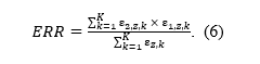
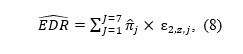
Selection for statistical significance is a well-known factor that distorts the published literature and challenges the cumulative progress in science. Recent replication failures have fueled concerns that many published results are false-positives. Brunner and Schimmack (2020) developed z-curve, a method for estimating the expected replication rate (ERR) – the predicted success rate of exact replication studies based on the mean power after selection for significance. This article introduces an extension of this method, z-curve 2.0. The main extension is an estimate of the expected discovery rate (EDR) – the estimate of a proportion that the reported statistically significant results constitute from all conducted statistical tests. This information can be used to detect and quantify the amount of selection bias by comparing the EDR to the observed discovery rate (ODR; observed proportion of statistically significant results). In addition, we examined the performance of bootstrapped confidence intervals in simulation studies. Based on these results, we created robust confidence intervals with good coverage across a wide range of scenarios to provide information about the uncertainty in EDR and ERR estimates. We implemented the method in the zcurve R package (Bartoš & Schimmack, 2020).
It has been known for decades that the published record in scientific journals is not representative of all studies that are conducted. For a number of reasons, most published studies are selected because they reported a theoretically interesting result that is statistically significant; p < .05 (Rosenthal & Gaito, 1964; Scheel, Schijen, & Lakens, 2021; Sterling, 1959; Sterling et al., 1995). This selective publishing of statistically significant results introduces a bias in the published literature. At the very least, published effect sizes are inflated. In the most extreme cases, a false-positive result is supported by a large number of statistically significant results (Rosenthal, 1979).
Some sciences (e.g., experimental psychology) tried to reduce the risk of false-positive results by demanding replication studies in multiple-study articles (cf. Wegner, 1992). However, internal replication studies provided a false sense of replicability because researchers used questionable research practices to produce successful internal replications (Francis, 2014; John, Lowenstein, & Prelec, 2012; Schimmack, 2012). The pervasive presence of publication bias at least partially explains replication failures in social psychology (Open Science Collaboration, 2015; Pashler & Wagenmakers, 2012, Schimmack, 2020); medicine (Begley & Ellis, 2012; Prinz, Schlange, & Asadullah 2011), and economics (Camerer et al., 2016; Chang & Li, 2015).
In meta-analyses, the problem of publication bias is usually addressed by one of the different methods for its detection and a subsequent adjustment of effect size estimates. However, many of them (Egger, Smith, Schneider, & Minder, 1997; Ioannidis and Trikalinos, 2007; Schimmack, 2012) perform poorly under conditions of heterogeneity (Renkewitz & Keiner, 2019), whereas others employ a meta-analytic model assuming that the studies are conducted on a single phenomenon (e.g., Hedges, 1992; Vevea & Hedges, 1995; Maier, Bartoš & Wagenmakers, in press). Moreover, while the aforementioned methods test for publication bias (return a p-value or a Bayes factor), they usually do not provide a quantitative estimate of selection bias. An exception would be the publication probabilities/ratios estimates from selection models (e.g., Hedges, 1992). Maximum likelihood selection models work well when the distribution of effect sizes is consistent with model assumptions, but can be biased when the distribution when the actual distribution does not match the expected distribution (e.g., Brunner & Schimmack, 2020; Hedges, 1992; Vevea & Hedges, 1995). Brunner and Schimmack (2020) introduced a new method that does not require a priori assumption about the distribution of effect sizes. The z-curve method uses a finite mixture model to correct for selection bias. We extended z-curve to also provide information about the amount of selection bias. To distinguish between the new and old z-curve methods, we refer to the old z-curve as z-curve 1.0 and the new z-curve as z-curve 2.0. Z-curve 2.0 has been implemented in the open statistic program R as the zcurve package that can be downloaded from CRAN (Bartoš & Schimmack, 2020).
Before we introduce z-curve 2.0, we would like to introduce some key statistical terms. We assume that readers are familiar with the basic concepts of statistical significance testing; normal distribution, null-hypothesis, alpha, type-I error, and false-positive result (see Bartoš & Maier, in press, for discussion of some of those concepts and their relation).
Glossary
Power is defined as the long-run relative frequency of statistically significant results in a series of exact replication studies with the same sample size when the null-hypothesis is false. For example, in a study with two groups (n = 50), a population effect size of Cohen’s d = 0.4 has 50.8% power to produce a statistically significant result. Thus, 100 replications of this study are expected to produce approximately 50 statistically significant results. The actual frequency will approach 50.8% as the study is repeated infinitely.
Unconditional power extends the concept of power to studies where the null-hypothesis is true. Typically, power is a conditional probability assuming a non-zero effect size (i.e., the null-hypothesis is false). However, the long-run relative frequency of statistically significant results is also known when the null-hypothesis is true. In this case, the long-run relative frequency is determined by the significance criterion, alpha. With alpha = 5%, we expect that 5 out of 100 studies will produce a statistically significant result. We use the term unconditional power to refer to the long-run frequency of statistically significant results without conditioning on a true effect. When the effect size is zero and alpha is 5%, unconditional power is 5%. As we only consider unconditional power in this article, we will use the term power to refer to unconditional power, just like Canadians use the term hockey to refer to ice hockey.
Mean (unconditional) power is a summary statistic of studies that vary in power. Mean power is simply the arithmetic mean of the power of individual studies. For example, two studies with power = .4 and power = .6, have a mean power of .5.
Discovery rate is a relative frequency of statistically significant results. Following Soric (1989), we call statistically significant results discoveries. For example, if 100 studies produce 36 statistically significant results, the discovery rate is 36%. Importantly, the discovery rate does not distinguish between true or false discoveries. If only false-positive results were reported, the discovery rate would be 100%, but none of the discoveries would reflect a true effect (Rosenthal, 1979).
Selection bias is a process that favors the publication of statistically significant results. Consequently, the published literature has a higher percentage of statistically significant results than was among the actually conducted studies. It results from significance testing that creates two classes of studies separated by the significance criterion alpha. Those with a statistically significant result, p < .05, where the null-hypothesis is rejected, and those with a statistically non-significant result, where the null-hypothesis is not rejected, p > .05. Selection for statistical significance limits the population of all studies that were conducted to the population of studies with statistically significant results. For example, if two studies produce p-values of .20 and .01, only the study with the p-value .01 is retained. Selection bias is often called publication bias. Studies show that authors are more likely to submit findings for publication when the results are statistically significant (Franco, Malhotra & Simonovits, 2014).
Observed discovery rate (ODR) is the percentage of statistically significant results in an observed set of studies. For example, if 100 published studies have 80 statistically significant results, the observed discovery rate is 80%. The observed discovery rate is higher than the true discovery rate when selection bias is present.
Expected discovery rate (EDR) is the mean power before selection for significance; in other words, the mean power of all conducted studies with statistically significant and non-significant results. As power is the long-run relative frequency of statistically significant results, the mean power before selection for significance is the expected relative frequency of statistically significant results. As we call statistically significant results discoveries, we refer to the expected percentage of statistically significant results as the expected discovery rate. For example, if we have two studies with power of .05 and .95, we are expecting 1 statistically significant result and an EDR of 50%, (.95 + .05)/2 = .5.
Expected replication rate (ERR) is the mean power after selection for significance, in other words, the mean power of only the statistically significant studies. Furthermore, since most people would declare a replication successful only if it produces a result in the same direction, we base ERR on the power to obtain a statistically significant result in the same direction. Using the prior example, we assume that the study with 5% power produced a statistically non-significant result and the study with 95% power produced a statistically significant result. In this case, we end up with only one statistically significant result with 95% power. Subsequently, the mean power after selection for significance is 95% (there is almost zero chance that a study with 95% power would produce replication with an outcome in the opposite direction). Based on this estimate, we would predict that 95% of exact replications of this study with the same sample size, and therefore with 95% power, will be statistically significant in the same direction.
As mean power after selection for significance predicts the relative frequency of statistically significant results in replication studies, we call it the expected replication rate. The ERR also corresponds to the “aggregate replication probability” discussed by Miller (2009).
Numerical Example
Before introducing the formal model, we illustrate the concepts with a fictional example. In the example, researchers test 100 true hypotheses with 100% power (i.e., every test of a true hypothesis produces p < .05) and 100 false hypotheses (H0 is true) with 5% power which is determined by alpha = .05. Consequently, the researchers obtain 100 true positive results and 5 false-positive results, for a total of 105 statistically significant results.[1] The expected discovery rate is (1 × 100 + 0.05 × 100)/(100 + 100) = 105/200 = 52.5% which corresponds to the observed discovery rate when all conducted studies are reported.
So far, we have assumed that there is no selection bias. However, let us now assume that 50 of the 95 statistically non-significant results are not reported. In this case, the observed discovery rate increased from 105/200 to 105/150 = 70%. The discrepancy between the EDR, 52.5%, and the ODR, 70%, provides quantitative information about the amount of selection bias.
As shown, the EDR provides valuable information about the typical power of studies and about the presence of selection bias. However, it does not provide information about the replicability of the statistically significant results. The reason is that studies with higher power are more likely to produce a statistically significant result in replications (Brunner & Schimmack, 2020; Miller, 2009). The main purpose of z-curve 1.0 was to estimate the mean power after selection for significance to predict the outcome of exact replication studies. In the example, only 5 of the 100 false hypotheses were statistically significant. In contrast, all 100 tests of the true hypothesis were statistically significant. This means that the mean power after selection for significance is (5 × .025 + 100 × 1)/(5 + 100) = 100.125/105 ≈ 95.4%, which is the expected replication rate.
Formal Introduction
Unfortunately, there is no standard symbol for power, which is usually denoted as 1 – β, with β being the probability of a type-II error. We propose to use epsilon, ε, as a Greek symbol for power because one Greek word for power starts with this letter (εξουσία). We further add subscript 1 or 2, depending on whether the direction of the outcome is relevant or not. Therefore, denotes power of a study regardless of the direction of the outcome and denotes power of a study in a specified direction.
The EDR,
is defined as the mean power (ε2) of a set of K studies, independent on the outcome direction.
Following Brunner and Schimmack (2020), the expected replication rate (ERR) is defined as the ratio of mean squared power and mean power of all studies, statistically significant and non-significant ones. We modify the definition here by taking the direction of the replication study into account.[2] The mean square power in the nominator is used because we are computing the expected relative frequency of statistically significant studies produced by a set of already statistically significant studies – if a study produces a statistically significant result with probability equal to its power, the chance that the same study will again be significant is power squared. The mean power in the denominator is used because we are restricting our selection to only already statistically significant studies which are produced at the rate corresponding to their power (see also Miller, 2009). The ratio simplifies by omitting division by K in both the nominator and denominator to:
which can also be read as a weighted mean power, where each power is weighted by itself. The weights originate from the fact that studies with higher power are more likely to produce statistically significant results. The weighted mean power of all studies is therefore equal to the unweighted mean power of the studies selected for significance (ksig; cf. Brunner & Schimmack, 2020).
If we have a set of studies with the same power (e.g., set of exact replications with the same sample size) that test for an effect with a z-test, the p-values converted to z-statistics follow a normal distribution with mean and a standard deviation equal to 1. Using an alpha level α, the power is the tail area of a standard normal distribution (Φ) centered over a mean, (μz) on the left and right side of the z-scores corresponding to alpha, -1.96 and 1.96 (with the usual alpha = .05),
or the tail area on the right side of the z-score corresponding to alpha, when we are also considering whether the directionality of the effect,
Two-sided p-values do not preserve the direction of the deviation from null and we cannot know whether a z-statistic comes from the lower or upper tail of the distribution. Therefore, we work with absolute values of z-statistics, changing their distribution from normal to folded normal distribution (Elandt, 1961; Leone, Nelson, & Nottingham, 1961).
Figure 1 illustrates the key concepts of z-curve with various examples. The first three density plots in the first row show the sampling distributions for studies with low (ε = 0.3), medium (ε = 0.5), and high (ε = .8) power, respectively. The last density plots illustrate the distribution that is obtained for a mixture of studies with low, medium, and high power with equal frequency (33.3% each). It is noteworthy that all four density distributions have different shapes. While Figure 1 illustrates how differences in power produce differences in the shape of the distributions, z-curve works backward and uses the shape of the distribution to estimate power.
Figure 1. Density (y-axis) of z-statistics (x-axis) generated by studies with different powers (columns) across different stages of the publication process (rows). The first row shows a distribution of z-statistics from z-tests homogeneous in power (the first three columns) or by their mixture (the fourth column). The second row shows only statistically significant z-statistics. The third row visualizes EDR as a proportion of statistically significant z-statistics out of all z-statistics. The fourth row shows a distribution of z-statistics from exact replications of only the statistically significant studies (dashed line for non-significant replication studies). The fifth row visualizes ERR as a proportion of statistically significant exact replications out of statistically significant studies.
Although z-curve can be used to fit the distributions in the first row, we assume that the observed distribution of all z-statistics is distorted by the selection bias. Even if some statistically non-significant p-values are reported, their distribution is subject to unknown selection effects. Therefore, by default z-curve assumes that selection bias is present and uses only the distribution of statistically significant results. This changes the distributions of z-statistics to folded normal distributions that are truncated at the z-score corresponding to the significance criterion, which is typically z = 1.96 for p = .05 (two-tailed). The second row in Figure 1 shows these truncated folded normal distributions. Importantly, studies with different levels of power produce different distributions despite the truncation. The different shapes of truncated distributions make it possible to estimate power by fitting a model to the truncated distribution. The third row of Figure 1 illustrates the EDR as a proportion of statistically significant studies from all conducted studies. We use Equation 3 to re-express EDR (Equation 2), which equals the mean unconditional power, of a set of K heterogenous studies using the means of sampling distributions of their z-statistics, μz,k,
Z-curve makes it possible to estimate the shape of the distribution in the region of statistically non-significant results on the basis of the observed distribution of statistically significant results. That is, after fitting a model to the grey area of the curve, it extrapolates the full distribution.
The fourth row of Figure 1 visualizes a distribution of expected z-statistics if the statistically significant studies were to be exactly replicated (not depicting the small proportion of results in the opposite direction than the original, significant, result). The full line highlights the portion of studies that would produce a statistically significant result, with the distribution of statistically non-significant studies drawn using the dashed line. An exact replication with the same sample size of the studies in the grey area in the second row is not expected to reproduce the truncated distribution again because truncation is a selection process. The replication distribution is not truncated and produces statistically significant and non-significant results. By modeling the selection process, z-curve predicts the non-truncated distributions in the fourth row from the truncated distributions in the second row.
The fifth row of Figure 1 visualizes ERR as a proportion of statistically significant exact replications in the expected direction from a set of the previously statistically significant studies. The ERR (Equation 1) of a set ofheterogeneous studies can be again re-expressed using Equations 3 and 4 with the means of sampling distributions of their z-statistics,
Z-curve 2.0
Z-curve is a finite mixture model (Brunner & Schimmack, 2020). Finite mixture models leverage the fact that an observed distribution of statistically significant z-statistics is a mixture of K truncated folded normal distribution with means and standard deviations 1. Instead of trying to estimate of every single observed z-statistic, a finite mixture model approximates the observed distribution based on K studies with a smaller set of J truncated folded normal distributions, , with J < K components,
Each mixture component j approximates a proportion of observed z-statistics with a probability density function, , of truncated folded normal distribution with parameters – a mean and standard deviation equal to 1. For example, while actual studies may vary in power from 40% to 60%, a mixture model may represent all of these studies with a single component with 50% power.
Z-curve 1.0 used three components with varying means. Extensive testing showed that varying means produced poor estimates of the EDR. Therefore, we switched to models with fixed means and increased the number of components to seven. The seven components are equally spaced by one standard deviation from z = 0 (power = alpha) to 6 (power ~ 1). As power for z-scores greater than 6 is essentially 1, it is not necessary to model the distribution of z-scores greater than 6, and all z-scores greater than 6 are assigned a power value of 1 (Brunner & Schimmack, 2020). The power values implied by the 7 components are .05, .17, .50, .85, .98, .999, .99997. We also tried a model with equal spacing of power, and we tried models with fewer or more components, but neither did improve performance in simulation studies.
We use the model parameter estimates to compute the estimated the EDR and ERR as the weighted average of seven truncated folded normal distributions centered over z = 0 to 6,
Curve Fitting
Z-curve 1.0 used an unorthodox approach to find the best fitting model that required fitting a truncated kernel-density distribution to the statistically significant z-statistics (Brunner & Schimmack, 2020). This is a non-trivial step that may produce some systematic bias in estimates. Z-curve 2.0 makes it possible to fit the model directly to the observed z-statistics using the well-established expectation maximization (EM) algorithm that is commonly used to fit mixture models (Dempster, Laird, & Rubin, 1977, Lee & Scott, 2012). Using the EM algorithm has the advantage that it is a well-validated method to fit mixture models. It is beyond the scope of this article to explain the mechanics of the EM algorithm (cf. Bishop, 2006), but it is important to point out some of its potential limitations. The main limitation is that it may terminate the search for the best fit before the best fitting model has been found. In order to prevent this, we run 20 searches with randomly selected starting values and terminate the algorithm in the first 100 iterations, or if the criterion falls below 1e-3. We then select the outcome with the highest likelihood value and continue until 1000 iterations or a criterion value of 1e-5 is reached. To speed up the fitting process, we optimized the procedure using Rcpp (Eddelbuettel et al., 2011).
Information about point estimates should be accompanied by information about uncertainty whenever possible. The most common way to do so is by providing confidence intervals. We followed the common practice of using bootstrapping to obtain confidence intervals for mixture models (Ujeh et al., 2016). As bootstrapping is a resource-intensive process, we used 500 samples for the simulation studies. Users of the z-curve package can use more iterations to analyze actual data.
Simulations
Brunner and Schimmack (2020) compared several methods for estimating mean power and found that z-curve performed better than three competing methods. However, these simulations were limited to the estimation of the ERR. Here we present new simulation studies to examine the performance of z-curve as a method to estimate the EDR as well. One simulation directly simulated power distributions, the other one simulated t-tests. We report the detailed results of both simulation studies in a Supplement. For the sake of brevity, we focus on the simulation of t-tests because readers can more easily evaluate the realism of these simulations. Moreover, most tests in psychology are t-tests or F-tests and Bruner and Schimmack (2020) already showed that the numerator degrees of freedom of F-tests do not influence results. Thus, the results for t-tests can be generalized to F-tests and z-tests.
The simulation was a complex 4 x 4 x 4 x 3 x 3 design with 576 cells. The first factor of the design that was manipulated was the mean effect size with Cohen’s ds ranging from 0 to 0.6 (0, 0.2, 0.4., 0.6). The second factor in the design was heterogeneity in effect sizes was simulated with a normal distribution around the mean effect size with SDs ranging from 0 to 0.6 (0, 0.2, 0.4., 0.6). Preliminary analysis with skewed distributions showed no influence of skew. The third factor of the design was sample size for between-subject design with N = 50, 100, and 200. The fourth factor of the design was the percentage of true null-hypotheses that ranged from 0 to 60% (0%, 20%, 40%, 60%). The last factor of the design was the number of studies with sets of k = 100, 300, and 1,000 statistically significant studies.
Each cell of the design was run 100 times for a total of 57,600 simulations. For the main effects of this design there were 57,600 / 4 = 14,400 or 57,600 / 3 = 19,200 simulations. Even for two-way interaction effects, the number of simulations is sufficient, 57,600 / 16 = 3,600. For higher interactions the design may be underpowered to detect smaller effects. Thus, our simulation study meets recommendations for sample sizes in simulation studies for main effects and two-way interactions, but not for more complex interaction effects (Morris, White, & Crowther, 2019). The code for the simulations is accessible at https://osf.io/r6ewt/.
Evaluation
For a comprehensive evaluation of z-curve 2.0 estimates, we report bias (i.e., mean distance between estimated and true values), root mean square error (RMSE; quantifying the error variance of the estimator), and confidence interval coverage (Morris et al. 2019).[3] To check the performance of the z-curve across different simulation settings, we analyzed the results of the factorial design using analyses of variance (ANOVAs) for continuous measures and logistic regression for the evaluation of confidence intervals (0 = true value not in the interval, 1 = true value in the interval). The analysis scripts and results are accessible at https://osf.io/r6ewt/.
Results
We start with the ERR because it is essentially a conceptual replication study of Brunner and Schimmack’s (2020) simulation studies with z-curve 1.0.
ERR
Visual inspection of the z-curves ERR estimates plotted against the true ERR values did not show any pathological behavior due to the approximation by a finite mixture model (Figure 3).
Figure 3. Estimated (y-axis) vs. true (x-axis) ERR in simulation U across a different number of studies.
Figure 3 shows that even with k = 100 studies, z-curve estimates are clustered close enough to the true values to provide useful predictions about the replicability of sets of studies. Overall bias was less than one percentage point, -0.88 (SEMCMC = 0.04). This confirms that z-curve has high large-sample accuracy (Brunner & Schimmack, 2020). RMSE decreased from 5.14 (SEMCMC = 0.03) percentage points with k = 100 to 2.21 (SEMCMC = 0.01) percentage points with k = 1,000. Thus, even with relatively small sample sizes of 100 studies, z-curve can provide useful information about the ERR.
The Analysis of Variance (ANOVA) showed no statistically significant 5-way interaction or 4-way interactions. A strong three-way interaction was found for effect size, heterogeneity of effect sizes, and sample size, z = 9.42. Despite the high statistical significance, effect sizes were small. Out of the 36 cells of the 4 x 3 x 3 design, 32 cells showed less than one percentage point bias. Larger biases were found when effect sizes were large, heterogeneity was low, and sample sizes were small. The largest bias was found for Cohen’s d = 0.6, SD = 0, and N = 50. In this condition, ERR was 4.41 (SEMCMC = 0.11) percentage points lower than the true replication rate. The finding that z-curve performs worse with low heterogeneity replicates findings by Brunner and Schimmack (2002). One reason could be that a model with seven components can easily be biased when most parameters are zero. The fixed components may also create a problem when true power is between two fixed levels. Although a bias of 4 percentage points is not ideal, it also does not undermine the value of a model that has very little bias across a wide range of scenarios.
The number of studies had a two-way interaction with effect size, z = 3.8, but bias in the 12 cells of the 4 x 3 design was always less than 2 percentage points. Overall, these results confirm the fairly good large sample accuracy of the ERR estimates.
We used logistic regression to examine patterns in the coverage of the 95% confidence intervals. This time a statistically significant four-way interaction emerged for effect size, heterogeneity of effect sizes, sample size, and the percentage of true null-hypotheses, z = 10.94. Problems mirrored the results for bias. Coverage was low when there were no true null-hypotheses, no heterogeneity in effect sizes, large effects, and small sample sizes. Coverage was only 31.3% (SEMCMC = 2.68) when the percentage of true H0 was 0, heterogeneity of effect sizes was 0, the effect size was Cohen’s d = 0.6, and the sample size was N = 50.
In statistics, it is common to replace confidence intervals that fail to show adequate coverage with confidence intervals that provide good coverage with real data; these confidence intervals are often called robust confidence intervals (Royall, 1996). We suspected that low coverage was related to systematic bias. When confidence intervals are drawn around systematically biased estimates, they are likely to miss the true effect size by the amount of systematic bias, when sampling error pushes estimates in the same direction as the systematic bias. To increase coverage, it is therefore necessary to take systematic bias into account. We created robust confidence intervals by adding three percentage points on each side. This is very conservative because the bias analysis would suggest that only adjustment in one direction is needed.
The logistic regression analysis still showed some statistically significant variation in coverage. The most notable finding was a 2-way interaction for effect size and sample size, z = 4.68. However, coverage was at 95% or higher for all 12 cells of the design. Further inspection showed that the main problem remained scenarios with high effect sizes (d = 0.6) and no heterogeneity (SD = 0), but even with small heterogeneity, SD = 0.2, this problem disappeared. We therefore recommend extending confidence intervals by three percentage points. This is the default setting in the z-curve package, but the package allows researchers to change these settings. Moreover, in meta-analyses of studies with low heterogeneity, alternative methods that are more appropriate for homogeneous methods (e.g., selection models; Hedges, 1992) may be used or the number of components could be reduced.
EDR
Visual inspection of EDRs plotted against the true discovery rates (Figure 4) showed a noticeable increase in uncertainty. This is to be expected as EDR estimates require estimation of the distribution for statistically non-significant z-statistics solely on the basis of the distribution of statistically significant results.
Figure 4. Estimated (y-axis) vs. true (x-axis) EDR across a different number of studies.
Despite the high variability in estimates, they can be useful. With the observed discovery rate in psychology being often over 90% (Sterling, 1959), many of these estimates would alert readers that selection bias is present. A bigger problem is that the highly variable EDR estimates might lack the power to detect selection bias in small sets of studies.
Across all studies, systematic bias was small, 1.42 (SEMCMC = 0.08) for 100 studies, 0.57 (SEMCMC = 0.06) for 300 studies, 0.16 (SEMCMC = 0.05) percentage points for 1000 studies. This shows that the shape of the distribution of statistically significant results does provide valid information about the shape of the full distribution. Consistent with Figure 4, RMSE values were large and remained fairly large even with larger number of studies, 11.70 (SEMCMC = 0.11) for 100 studies, 8.88 (SEMCMC = 0.08) for 300 studies, 6.49 (SEMCMC = 0.07) percentage points for 1000 studies. These results show how costly selection bias is because more precise estimates of the discovery rate would be available without selection bias.
The main consequence of high RMSE is that confidence intervals are expected to be wide. The next analysis examined whether confidence intervals have adequate coverage. This was not the case; coverage = 87.3% (SEMCMC = 0.14). We next used logistic regression to examine patterns in coverage in our simulation design. A notable 3-way interaction between effect size, sample size, and percentage of true H0 was present, z = 3.83. While the pattern was complex, not a single cell of the design showed coverage over 95%.
As before, we created robust confidence intervals by extending the interval. We settled for an extension by five percentage points. The 3-way interaction remained statistically significant, z = 3.36. Now 43 of the 48 cells showed coverage over 95%. For reasons that are not clear to us, the main problem occurred for an effect size of Cohen’s d = 0.4 and no true H0, independent of sample size. While improving the performance of z-curve remains an important goal and future research might find better approaches to address this problem, for now, we recommend using z-curve 2.0 with these robust confidence intervals, but users can specify more conservative adjustments.
Application to Real Data
It is not easy to evaluate the performance of z-curve 2.0 estimates with actual data because selection bias is ubiquitous and direct replication studies are fairly rare (Zwaan, Etz, Lucas, & Donnellan, 2018). A notable exception is the Open Science Collaboration project that replicated 100 studies from three psychology journals (Open Science Collaboration, 2015). This unprecedented effort has attracted attention within and outside of psychological science and the article has already been cited over 1,000 times. The key finding was that out of 97 statistically significant results, including marginally significant ones, only 36 replication studies (37%) reproduced a statistically significant result in the replication attempts.
This finding has produced a wide range of reactions. Often the results are cited as evidence for a replication crisis in psychological science, especially social psychology (Schimmack, 2020). Others argue that the replication studies were poorly carried out and that many of the original results are robust findings (Bressan, 2019). This debate mirrors other disputes about failures to replicate original results. The interpretation of replication studies is often strongly influenced by researchers’ a priori beliefs. Thus, they rarely settle academic disputes. Z-curve analysis can provide valuable information to determine whether an original or a replication study is more trustworthy. If a z-curve analysis shows no evidence for selection bias and a high ERR, it is likely that the original result is credible and the replication failure is a false negative result or the replication study failed to reproduce the original experiment. On the other hand, if there is evidence for selection bias and the ERR is low, replication failures are expected because the original results were obtained with questionable research practices.
Another advantage of z-curve analyses of published results is that it is easier to obtain large representative samples of studies than to conduct actual replication studies. To illustrate the usefulness of z-curve analyses, we focus on social psychology because this field has received the most attention from meta-psychologists (Schimmack, 2020). We fitted z-curve 2.0 to two studies of published test statistics from social psychology and compared these results to the actual success rate in the Open Science Collaboration project (k = 55).
One sample is based on Motyl et al.’s (2017) assessment of the replicability of social psychology (k = 678). The other sample is based on the coding of the most highly cited articles by social psychologists with a high H-Index (k = 2,208; Schimmack, 2021). The ERR estimates were 44%, 95% CI [35, 52]%, and 51%, 95% CI [45, 56]%. The two estimates do not differ significantly from each other, but both estimates are considerably higher than the actual discovery rate in the OSC replication project, 25%, 95% CI [13, 37]%. We postpone the discussion of this discrepancy to the discussion section.
The EDRs estimates were 16%, 95% CI [5, 32]%, and 14%, 95% CI [7, 23]%. Again, both of the estimates overlap and do not significantly differ. At the same time, the EDR estimates are much lower than the ODRs in these two data sets (90%, 89%). The z-curve analysis of published results in social psychology shows a strong selection bias that explains replication failures in actual replication attempts. Thus, the z-curve analysis reveals that replication failures cannot be attributed to problems of the replication attempts. Instead, the low EDR estimates show that many non-significant original results are missing from the published record.
Discussion
A previous article introduced z-curve as a viable method to estimate mean power after selection for significance (Brunner & Schimmack, 2020). This is a useful statistic because it predicts the success rate of exact replication studies. We therefore call this statistic the expected replication rate. Studies with a high replication rate provide credible evidence for a phenomenon. In contrast, studies with a low replication rate are untrustworthy and require additional evidence.
We extended z-curve 1.0 in two ways. First, we implemented the expectation maximization algorithm to fit the mixture model to the observed distribution of z-statistics. This is a more conventional method to fit mixture models. We found that this method produces good estimates, but it did not eliminate some of the systematic biases that were observed with z-curve 1.0. More important, we extended z-curve to estimate the mean power before selection for significance. We call this statistic the expected discovery rate because mean power predicts the percentage of statistically significant results for a set of studies. We found that EDR estimates have satisfactory large sample accuracy, but vary widely in smaller sets of studies. This limits the usefulness for meta-analysis of small sets of studies, but as we demonstrated with actual data, the results are useful when a large set of studies is available. The comparison of the EDR and ODR can also be used to assess the amount of selection bias. A low EDR can also help researchers to realize that they test too many false hypotheses or test true hypotheses with insufficient power.
In contrast to Miller (2009), who stipulates that estimating the ERR (“aggregated replication probability”) is unattainable due to selection processes, Schimmack and Brunner’s (2020) z-curve 1.0 addresses the issue by modeling the selection for significance.
Finally, we examined the performance of bootstrapped confidence intervals in simulation studies. We found that coverage for 95% confidence intervals was sometimes below 95%. To improve the coverage of confidence intervals, we created robust confidence intervals that added three percentage points to the confidence interval of the ERR and five percentage points to the confidence interval of the EDR.
We demonstrate the usefulness of the EDR and confidence intervals with an example from social psychology. We find that ERR overestimates the actual replicability in social psychology. We also find clear evidence that power in social psychology is low and that high success rates are mostly due to selection for significance. It is noteworthy that while the Motyl et al.’s (2017) dataset is representative for social psychology, Schimmack’s (2021) dataset sampled highly influential articles. The fact that both sampling procedures produced similar results suggests that studies by eminent researchers or studies with high citation rates are no more replicable than other studies published in social psychology.
Z-curve 2.0 does provide additional valuable information that was not provided by z-curve 1.0. Moreover, z-curve 2.0 is available as an R-package, making it easier for researchers to conduct z-curve analyses (Bartoš & Schimmack, 2020). This article provides the theoretical background for the use of the z-curve package. Subsequently, we discuss some potential limitations of z-curve 2.0 analysis and compare z-curve 2.0 to other methods that aim to estimate selection bias or power of studies.
Bias Detection Methods
In theory, bias detection is as old as meta-analysis. The first bias test showed that Mendel’s genetic experiments with peas had less sampling error than a statistical model would predict (Pires & Branco, 2010). However, when meta-analysis emerged as a widely used tool to integrate research findings, selection bias was often ignored. Psychologists focused on fail-safe N (Rosenthal, 1979), which did not test for the presence of bias and often led to false conclusions about the credibility of a result (Ferguson & Heene, 2012). The most common tools to detect bias rely on correlations between effect sizes and sample size. A key problem with this approach is that it often has low power and that results are not trustworthy under conditions of heterogeneity (Inzlicht, Gervais, & Berkman, 2015; Renkewitz & Keiner, 2019). The tests are also not useful for meta-analysis of heterogeneous sets of studies where researchers use larger samples to study smaller effects, which also introduces a correlation between effect sizes and sample sizes. Due to these limitations, evidence of bias has been dismissed as inconclusive (Cunningham & Baumeister, 2016; Inzlicht & Friese; 2019).
It is harder to dismiss evidence of bias when a set of published studies has more statistically significant results than the power of the studies warrants; that is, the ODR exceeds the EDR (Sterling et al., 1995). Aside from z-curve 2.0, there are two other bias tests that rely on a comparison of the ODR and EDR to evaluate the presence of selection bias, namely the Test of Excessive Significance (TES, Ioannidis & Trikalinos, 2005) and the Incredibility Test (IT; Schimmack, 2012).
Z-curve 2.0 has several advantages over the existing methods. First, TES was explicitly designed for meta-analysis with little heterogeneity and may produce biased results when heterogeneity is present (Renkewitz & Keiner, 2019). Second, both the TES and the IT take observed power at face value. As observed power is inflated by selection for significance, the tests have low power to detect selection for significance, unless the selection bias is large. Finally, TES and IT rely on p-values to provide information about bias. As a result, they do not provide information about the amount of selection bias.
Z-curve 2.0 overcomes these problems by correcting the power estimate for selection bias, providing quantitative evidence about the amount of bias by comparing the ODR and EDR, and by providing evidence about statistical significance by means of a confidence interval around the EDR estimate. Thus, z-curve 2.0 is a valuable tool for meta-analysts, especially when analyzing a large sample of heterogenous studies that vary widely in designs and effect sizes. As we demonstrated with our example, the EDR of social psychology studies is very low. This information is useful because it alerts readers to the fact that not all p-values below .05 reveal a true and replicable finding.
Nevertheless, z-curve has some limitations. One limitation is that it does not distinguish between significant results with opposite signs. In the presence of multiple tests of the same hypothesis with opposite signs, researchers can exclude inconsistent significant results and estimate z-curve on the basis of significant results with the correct sign. However, the selection of tests by the meta-analyst introduces additional selection bias, which has to be taken into account in the comparison of the EDR and ODR. Another limitation is the assumption that all studies used the same alpha criterion (.05) to select for significance. This possibility can be explored by conducting multiple z-curve analyses with different selection criteria (e.g., .05, .01). The use of lower selection criteria is also useful because some questionable research practices produce a cluster of just significant results. However, all statistical methods can only produce estimates that come with some uncertainty. When severe selection bias is present, new studies are needed to provide credible evidence for a phenomenon.
Predicting Replication Outcomes
Since 2011, many psychologists have learned that published significant results can have a low replication probability (Open Science Collaboration, 2015). This makes it difficult to trust the published literature, especially older articles that report results from studies with small samples that were not pre-registered. Should these results be disregarded because they might have been obtained with questionable research practices? Should results only be trusted if they have been replicated in a new, ideally pre-registered, replication study? Or should we simply assume that most published results are probably true and continue to treat every p-value below .05 as a true discovery?
The appeal of z-curve is that we can use the published evidence to distinguish between credible and “incredible” (biased) statistically significant results. If a meta-analysis shows low selection bias and a high replication rate, the results are credible. If a meta-analysis shows high selection bias and a low replication rate, the results are incredible and require independent verification.
As appealing as this sounds, every method needs to be validated before it can be applied to answer substantive questions. This is also true for z-curve 2.0. We used the results from the OSC replicability project for this purpose. The results suggest that z-curve predictions of replication rates may be overly optimistic. While the expected replication rate was between 44% and 51% (35% – 56% CI range), the actual success rate was only 25%, 95% CI [13, 37]%. Thus, it is important to examine why z-curve estimates are higher than the actual replication rate in the OSC project.
One possible explanation is that there is a problem with the replication studies. Social psychologists quickly criticized the quality of the replication studies (Gilbert, King, Pettigrew, & Wilson, 2016). In response, the replication team conducted the new replications of contested replication studies. Based on the effect sizes in these much larger replication studies, not a single original study would have produced statistically significant results (Ebersole et al., 2020). It is therefore unlikely that the quality of replication studies explains the low success rate of replication studies in social psychology.
A more interesting explanation is that social psychological phenomena are not as stable as boiling distilled water under tightly controlled laboratory conditions. Rather, effect sizes vary across populations, experimenters, times of day, and a myriad of other factors that are difficult to control (Stroebe & Strack, 2014). In this case, selection for significance produces additional regression to the mean because statistically significant results were obtained with the help of favorable hidden moderators that produced larger effect sizes that are unlikely to be present again in a direct replication study.
The worst-case scenario is that studies that were selected for significance are no more powerful than studies that produced statistically non-significant results. In this case, the EDR predicts the outcome of actual replication studies. Consistent with this explanation, the actual replication rate of 25%, 95% CI [13, 37]%, was highly consistent with the EDR estimates of 16%, 95% CI [5, 32]%, and 14%, 95% CI [7, 23]%. More research is needed once more replication studies become available to see how closely actual replication rates are to the EDR and the ERR. For now, they should be considered the worst and the best possible scenarios and actual replication rates are expected to fall somewhere between these two estimates.
A third possibility for the discrepancy is that questionable research practices change the shape of the z-curve in ways that are different from a simple selection model. For example, if researchers have several statistically significant results and pick the highest one, the selection model underestimates the amount of selection that occurred. This can bias z-curve estimates and inflate the ERR and EDR estimates. Unfortunately, it is also possible that questionable research practices have the opposite effect and that ERR and EDR estimates underestimate the true values. This uncertainty does not undermine the usefulness of z-curve analyses. Rather it shows how questionable research practices undermine the credibility of published results. Z-curve 2.0 does not alleviate the need to reform research practices and to ensure that all researchers report their results honestly.
Conclusion
Z-curve 1.0 made it possible to estimate the replication rate of a set of studies on the basis of published test results. Z-curve 2.0 makes it possible to also estimate the expected discovery rate; that is, how many tests were conducted to produce the statistically significant results. The EDR can be used to evaluate the presence and amount of selection bias. Although there are many methods that have the same purpose, z-curve 2.0 has several advantages over these methods. Most importantly, it quantifies the amount of selection bias. This information is particularly useful when meta-analyses report effect sizes based on methods that do not consider the presence of selection bias.
Author Contributions
Most of the ideas in the manuscript were developed jointly. The main idea behind the z-curve method and its density version was developed by Dr. Schimmack. Mr. Bartoš implemented the EM version of the method and conducted the extensive simulation studies.
Acknowledgments
Access to computing and storage facilities owned by parties and projects contributing to the National Grid Infrastructure MetaCentrum provided under the program “Projects of Large Research, Development, and Innovations Infrastructures” (CESNET LM2015042), is greatly appreciated. We would like to thank Maximilian Maier, Erik W. van Zwet, and Leonardo Tozzi for valuable comments on a draft of this manuscript.
No conflict of interest to report. This work was not supported by a specific grant.
References
Bartoš, F., & Maier, M. (in press). Power or alpha? The better way of decreasing the false discovery rate. Meta-Psychology. https://doi.org/10.31234/osf.io/ev29a
Bartoš, F., & Schimmack, U. (2020). “zcurve: An R Package for Fitting Z-curves.” R package version 1.0.0
Begley, C. G., & Ellis, L. M. (2012). Raise standards for preclinical cancer research. Nature, 483(7391), 531–533. https://doi.org/10.1038/483531a
Bishop, C. M. (2006). Pattern recognition and machine learning. Springer.
Boos, D. D., & Stefanski, L. A. (2011). P-value precision and reproducibility. The American Statistician, 65(4), 213-221. https://doi.org/10.1198/tas.2011.10129
Brunner, J. & Schimmack, U. (2020). Estimating population mean power under conditions of heterogeneity and selection for significance. Meta-Psychology, 4, https://doi.org/10.15626/MP.2018.874
Camerer, C. F., Dreber, A., Forsell, E., Ho, T. H., Huber, J., Johannesson, M., … & Heikensten, E. (2016). Evaluating replicability of laboratory experiments in economics. Science, 351(6280). https://doi.org/10.1126/science.aaf0918
Chang, Andrew C., and Phillip Li (2015). Is economics research replicable? Sixty published papers from thirteen journals say ”usually not”, Finance and Economics Discussion Series 2015-083. Washington: Board of Governors of the Federal Reserve System. http://dx.doi.org/10.17016/FEDS.2015.083.
Chase, L. J., & Chase, R. B. (1976). Statistical power analysis of applied psychological research. Journal of Applied Psychology, 61(2), 234–237. https://doi.org/10.1037/0021-9010.61.2.234
Cunningham, M. R., & Baumeister, R. F. (2016). How to make nothing out of something: Analyses of the impact of study sampling and statistical interpretation in misleading meta-analytic conclusions. Frontiers in Psychology, 7, 1639. https://doi.org/10.3389/fpsyg.2016.01639
Dempster, A. P., Laird, N. M., & Rubin, D. B. (1977). Maximum likelihood from incomplete data via the EM algorithm. Journal of the Royal Statistical Society: Series B (Methodological), 39(1), 1–22. https://doi.org/10.1111/j.2517-6161.1977.tb01600.x
Ebersole, C. R., Mathur, M. B., Baranski, E., Bart-Plange, D.-J., Buttrick, N. R., Chartier, C. R., Corker, K. S., Corley, M., Hartshorne, J. K., IJzerman, H., Lazarević, L. B., Rabagliati, H., Ropovik, I., Aczel, B., Aeschbach, L. F., Andrighetto, L., Arnal, J. D., Arrow, H., Babincak, P., … Nosek, B. A. (2020). Many Labs 5: Testing pre-data-collection peer review as an intervention to increase replicability. Advances in Methods and Practices in Psychological Science, 3(3), 309–331. https://doi.org/10.1177/2515245920958687
Egger, M., Smith, G. D., Schneider, M., & Minder, C. (1997). Bias in meta-analysis detected by a simple, graphical test. BMJ,315(7109), 629-634. https://doi.org/10.1136/bmj.315.7109.629
Eddelbuettel, D., François, R., Allaire, J., Ushey, K., Kou, Q., Russel, N., … Bates, D. (2011). Rcpp: Seamless R and C++ integration. Journal of Statistical Software, 40(8), 1–18. https://doi.org/10.18637/jss.v040.i08
Elandt, R. C. (1961). The folded normal distribution: Two methods of estimating parameters from moments. Technometrics, 3(4), 551–562. https://doi.org/10.2307/1266561
Ferguson, C. J., & Heene, M. (2012). A vast graveyard of undead theories: Publication bias and psychological science’s aversion to the null. Perspectives on Psychological Science, 7(6), 555–561. https://doi.org/10.1177/1745691612459059
Francis G., (2014). The frequency of excess success for articles in Psychological Science. Psychonomic Bulletin and Review, 21, 1180–1187. https://doi.org/10.3758/s13423-014-0601-x
Franco, A., Malhotra, N., & Simonovits, G. (2014). Publication bias in the social sciences: Unlocking the file drawer. Science, 345(6203), 1502-1505. . https://doi.org/10.1126/science.1255484
Gilbert, D. T., King, G., Pettigrew, S., & Wilson, T. D. (2016). Comment on “Estimating the reproducibility of psychological science.” Science,351, 1037–1103. http://dx.doi.org/10.1126/science.aad7243
Hedges, L. V. (1992). Modeling publication selection effects in meta-analysis. Statistical Science,7(2), 246–255. https://doi.org/10.1214/ss/1177011364
Inzlicht, M., Gervais, W., & Berkman, E. (2015). Bias-correction techniques alone cannot determine whether ego depletion is different from zero: Commentary on Carter, Kofler, Forster, & McCullough, 2015. Kofler, Forster, & McCullough. http://dx.doi.org/10.2139/ssrn.2659409
Ioannidis, J. P., & Trikalinos, T. A. (2007). An exploratory test for an excess of significant findings. Clinical Trials, 4(3), 245–253. https://doi.org/10.1177/1740774507079441
John, L. K., Lowenstein, G., & Prelec, D. (2012). Measuring the prevalence of questionable research practices with incentives for truth telling. Psychological Science, 23, 517–523. https://doi.org/10.1177/0956797611430953
Lee, G., & Scott, C. (2012). EM algorithms for multivariate Gaussian mixture models with truncated and censored data. Computational Statistics & Data Analysis, 56(9), 2816–2829. https://doi.org/10.1016/j.csda.2012.03.003
Maier, M., Bartoš, F., & Wagenmakers, E. (in press). Robust Bayesian meta-analysis: Addressing publication bias with model-averaging. Psychological Methods. https://doi.org/10.31234/osf.io/u4cns
Miller, J. (2009). What is the probability of replicating a statistically significant effect?. Psychonomic Bulletin & Review 16, 617–640. https://doi.org/10.3758/PBR.16.4.617
Morris, T. P., White, I. R., & Crowther, M. J. (2019). Using simulation studies to evaluate statistical methods. Statistics in Medicine, 38(11), 2074-2102. https://doi.org/10.1002/sim.8086
Motyl, M., Demos, A. P., Carsel, T. S., Hanson, B. E., Melton, Z. J., Mueller, A. B., Prims, J. P., Sun, J., Washburn, A. N., Wong, K. M., Yantis, C., & Skitka, L. J. (2017). The state of social and personality science: Rotten to the core, not so bad, getting better, or getting worse? Journal of Personality and Social Psychology, 113(1), 34–58. https://doi.org/10.1037/pspa0000084
Open Science Collaboration. (2015). Estimating the reproducibility of psychological science. Science, 349(6251), aac4716–aac4716. https://doi.org/10.1126/science.aac4716
Pashler, H., & Wagenmakers, E. J. (2012). Editors’ introduction to the special section on replicability in psychological science: A crisis of confidence? Perspectives on Psychological Science, 7(6), 528-530. https://doi.org/10.1177/1745691612465253
Pires, A. M., & Branco, J. A. (2010). A statistical model to explain the Mendel—Fisher controversy. Statistical Science, 545-565. https://doi.org/10.1214/10-STS342
Prinz, F., Schlange, T., & Asadullah, K. (2011). Believe it or not: how much can we rely on published data on potential drug targets? Nature Reviews Drug Discovery, 10(9), 712–712. https://doi.org/10.1038/nrd3439-c1
Renkewitz, F., & Keiner, M. (2019). How to detect publication bias in psychological research. Zeitschrift für Psychologie. https://doi.org/10.1027/2151-2604/a000386
Rosenthal, R., & Gaito, J. (1964). Further evidence for the cliff effect in interpretation of levels of significance. Psychological Reports 15(2), 570.https://doi.org/10.2466/pr0.1964.15.2.570
Scheel, A. M., Schijen, M. R., & Lakens, D. (2021). An excess of positive results: Comparing the standard Psychology literature with Registered Reports. Advances in Methods and Practices in Psychological Science, 4(2), https://doi.org/10.1177/25152459211007467
Schimmack, U. (2012). The ironic effect of significant results on the credibility of multiple-study articles. Psychological Methods, 17, 551–566. https://doi.org/10.1037/a0029487
Schimmack, U. (2020). A meta-psychological perspective on the decade of replication failures in social psychology. Canadian Psychology/Psychologie canadienne. 61 (4), 364-376. https://doi.org/10.1037/cap0000246
Sorić, B. (1989). Statistical “discoveries” and effect-size estimation. Journal of the American Statistical Association, 84(406), 608-610. https://doi.org/10.2307/2289950
Sterling, T. D. (1959). Publication decision and the possible effects on inferences drawn from tests of significance – or vice versa. Journal of the American Statistical Association, 54, 30–34. https://doi.org/10.2307/2282137
Sterling, T. D., Rosenbaum, W. L., & Weinkam, J. J. (1995). Publication decisions revisited: The effect of the outcome of statistical tests on the decision to publish and vice versa. The American Statistician, 49, 108–112. https://doi.org/10.2307/2684823
Stroebe, W., & Strack, F. (2014). The alleged crisis and the illusion of exact replication. Perspectives on Psychological Science, 9, 59–71. http://dx.doi.org/10.1177/1745691613514450
Vevea, J. L., & Hedges, L. V. (1995). A general linear model for estimating effect size in the presence of publication bias. Psychometrika, 60(3), 419–435. https://doi.org/10.1007/BF02294384
Wegner, D. M. (1992). The premature demise of the solo experiment. Personality and Social Psychology Bulletin, 18(4), 504-508. https://doi.org/10.1177/0146167292184017
Zwaan, R. A., Etz, A., Lucas, R. E., & Donnellan, M. B. (2018). Making replication mainstream. Behavioral and Brain Sciences, 41, Article e120. https://doi.org/10.1017/S0140525X17001972
Footnotes
[1] In reality, sampling erorr will produce an observed discovery rate that deviates slightly from the expected discovery rate. To keep things simple, we assume that the observed discovery rate matches the expected discovery rate perfectly.
[2] We thank Erik van Zwet for suggesting this modification in his review and for many other helpful comments.
[3] To compute MCMC standard errors of bias and RMSE across multiple conditions with different true ERR/EDR value, we centered the estimates by substracting the true ERR/EDR. For computing the MCMC standard error of RMSE, we used the Jackknife estimate of variance Efron & Stein (1981).
This blog post is heavily based on one of my first blog-posts in 2014 (Schimmack, 2014). The blog post reports a meta-analysis of ego-depletion studies that used the hand-grip paradigm. When I first heard about the hand-grip paradigm, I thought it was stupid because there is so much between-subject variance in physical strength. However, then I learned that it is the only paradigm that uses a pre-post design, which removes between-subject variance from the error term. This made the hand-grip paradigm the most interesting paradigm because it has the highest power to detect ego-depletion effects. I conducted a meta-analysis of the hand-grip studies and found clear evidence of publication bias. This finding is very damaging to the wider ego-depletion research because other studies used between-subject designs with small samples which have very low power to detect small effects.
This prediction was confirmed in meta-analyses by Carter,E.C., Kofler, L.M., Forster, D.E., and McCulloch,M.E. (2015) that revealed publication bias in ego-depletion studies with other paradigms.
The results also explain why attempts to show ego-depletion effects with within-subject designs failed (Francis et al., 2018). Within-subject designs increase power by removing fixed between-subject variance such as physical strength. However, given the lack of evidence with the hand-grip paradigm it is not surprising that within-subject designs also failed to show ego-depletion effects with other dependent variables in within-subject designs. Thus, these results further suggest that ego-depletion effects are too small to be used for experimental investigations of will-power.
Of course, Roy F. Baumeister doesn’t like this conclusion because his reputation is to a large extent based on the resource model of will-power. His response to the evidence that most of the evidence is based on questionable practices that produced illusory evidence has been to attack the critics (cf. Schimmack, 2019).
In 2016, he paid to publish a critique of Carter’s (2015) meta-analysis in Frontiers of Psychology (Cunningham & Baumeister, 2016). In this article, the authors question the results obtained by bias-tests that reveal publication bias and suggest that there is no evidence for ego-depletion effects.
Unfortunately, Cunningham and Baumeister’s (2016) article is cited frequently as if it contained some valid scientific arguments.
For example, Christodoulou, Lac, and Moore (2017) cite the article to dismiss the results of a PEESE analysis that suggests publication bias is present and there is no evidence that infants can add and subtract. Thus, there is a real danger that meta-analysts will use Cunningham & Baumeister’s (2016) article to dismiss evidence of publication bias and to provide false evidence for claims that rest on questionable research practices.
Fact Checking Cunningham and Baumeister’s Criticisms
Cunningham and Baumeister (2016) claim that results from bias tests are difficult to interpret, but there criticism is based on false arguments and inaccurate claims.
Confusing Samples and Populations
This scientifically sounding paragraph is a load of bull. The authors claim that inferential tests require sampling from a population and raise a question about the adequacy of a sample. However, bias tests do not work this way. They are tests of the population, namely the population of all of the studies that could be retrieved that tested a common hypothesis (e.g., all handgrip studies of ego-depletion). Maybe more studies exist than are available. Maybe the results based on the available studies differ from results if all studies were available, but that is irrelevant. The question is only whether the available studies are biased or not. So, why do we even test for significance? That is a good question. The test for significance only tells us whether bias is merely a product of random chance or whether it was introduced by questionable research practices. However, even random bias is bias. If a set of studies reports only significant results, and the observed power of the studies is only 70%, there is a discrepancy. If this discrepancy is not statistically significant, there is still a discrepancy. If it is statistically significant, we are allowed to attribute it to questionable research practices such as those that Baumeister and several others admitted using.
“We did run multiple studies, some of which did not work, and some of which worked better than others. You may think that not reporting the less successful studies is wrong, but that is how the field works.” (Roy Baumeister, personal email communication) (Schimmack, 2014).
Given the widespread use of questionable research practices in experimental social psychology, it is not surprising that bias-tests reveal bias. It is actually more surprising when these tests fail to reveal bias, which is most likely a problem of low statistical power (Renkewitz & Keiner, 2019).
Misunderstanding Power
The claims about power are not based on clearly defined constructs in statistics. Statistical power is a function of the strength of a signal (the population effect size) and the amount of noise (sampling error). Researches skills are not a part of statistical power. Results should be independent of a researcher. A researcher could of course pick procedures that maximize a signal (powerful interventions) or reduce sampling error (e.g., pre-post designs), but these factors play a role in the designing of a study. Once a study is carried out, the population effect size is what it was and the sampling error is what it was. Thus, honestly reported test statistics tell us about the signal-to-noise ratio in a study that was conducted. Skillful researchers would produce stronger test-statistics (higher t-values, F-values) than unskilled researchers. The problem for Baumeister and other ego-depletion researchers is that the t-values and F-values tend to be weak and suggest questionable research practices rather than skill produced significant results. In short, meta-analysis of test-statistics reveal whether researchers used skill or questionable research practices to produce significant results.
The reference to Morey (2013) suggests that there is a valid criticism of bias tests, but that is not the case. Power-based bias tests are based on sound statistical principles that were outlined by a statistician in the journal American Statistician (Sterling, Rosenbaum, & Weinkam, 1995). Building on this work, Jerry Brunner (professor of statistics) and I published theorems that provide the basis of bias tests like TES to reveal the use of questionable research practices (Brunner & Schimmack, 2019). The real challenge for bias tests is to estimate mean power without information about the population effect sizes. In this regard, TES is extremely conservative because it relies on a meta-analysis of observed effect sizes to estimate power. These effect sizes are inflated when questionable research practices were used, which makes the test conservative. However, there is a problem with TES when effect sizes are heterogeneous. This problem is avoided by alternative bias tests like the R-Index that I used to demonstrate publication bias in the handgrip studies of ego-depletion. In sum, bias tests like the R-Index and TES are based on solid mathematical foundations and simulation studies show that they work well in detecting the use of questionable research practices.
Confusing Absence of Evidence with Evidence of Absence
PET and PEESE are extension of Eggert’s regression test of publication bias. All methods relate sample sizes (or sampling error) to effect size estimates. Questionable research practices tend to introduce a negative correlation between sample size and effect sizes or a positive correlation between sampling error and effect sizes. The reason is that significance requires a signal to noise ratio of 2:1 for t-tests or 4:1 for F-tests to produce a significant result. To achieve this ratio with more noise (smaller sample, more sampling error), the signal has to be inflated more.
The novel contribution of PET and PEESE was to use the intercept of the regression model as an effect size estimate that corrects for publication bias. This estimate needs to be interpreted in the context of the sampling error of the regression model, using a 95%CI around the point estimate.
Carter et al. (2015) found that the 95%CI often included a value of zero, which implies that the data are too weak to reject the null-hypothesis. Such non-significant results are notoriously difficult to interpret because they neither support nor refute the null-hypothesis. The main conclusion that can be drawn from this finding is that the existing data are inconclusive.
This main conclusion does not change when the number of studies is less than 20. Stanley and Doucouliagos (2014) were commenting on the trustworthiness of point estimates and confidence intervals in smaller samples. Smaller samples introduce more uncertainty and we should be cautious in the interpretation of results that suggest there is an effect because the assumptions of the model are violated. However, if the results already show that there is no evidence, small samples merely further increase uncertainty and make the existing evidence even less conclusive.
Aside from the issues regarding the interpretation of the intercept, Cunningham and Baumeister also fail to address the finding that sample sizes and effect sizes were negatively correlated. If this negative correlation is not caused by questionable research practices, it must be caused by something else. Cunningham and Baumeister fail to provide an answer to this important question.
No Evidence of Flair and Skill
Earlier Cunningham and Baumeister (2016) claimed that power depends on researchers’ skills and they argue that new investigators may be less skilled than the experts who developed paradigms like Baumeister and colleagues.
However, they then point out that Carter et al.’s (2015) examined lab as a moderator and found no difference between studies conducted by Baumeister and colleagues or other laboratories.
Thus, there is no evidence whatsoever that Baumeister and colleagues were more skillful and produced more credible evidence for ego-depletion than other laboratories. The fact that everybody got ego-depletion effects can be attributed to the widespread use of questionable research practices that made it possible to get significant results even for implausible phenomena like extrasensory perception (John et al., 2012; Schimmack, 2012). Thus, the large number of studies that support ego-depletion merely shows that everybody used questionable research practices like Baumeister did (Schimmack, 2014; Schimmack, 2016), which is also true for many other areas of research in experimental social psychology (Schimmack, 2019). Francis (2014) found that 80% of articles showed evidence that QRPs were used.
Handgrip Replicability Analysis
The meta-analysis included 18 effect sizes based on handgrip studies. Two unpublished studies (Ns = 24, 37) were not included in this analysis. Seeley & Gardner (2003)’s study was excluded because it failed to use a pre-post design, which could explain the non-significant result. The meta-analysis reported two effect sizes for this study. Thus, 4 effects were excluded and the analysis below is based on the remaining 14 studies.
All articles presented significant effects of will-power manipulations on handgrip performance. Bray et al. (2008) reported three tests; one was deemed not significant (p = .10), one marginally significant (.06), and one was significant at p = .05 (p = .01). The results from the lowest p-value were used. As a result, the success rate was 100%.
Median observed power was 63%. The inflation rate is 37% and the R-Index is 26%. An R-Index of 22% is consistent with a scenario in which the null-hypothesis is true and all reported findings are type-I errors. Thus, the R-Index supports Carter and McCullough’s (2014) conclusion that the existing evidence does not provide empirical support for the hypothesis that will-power manipulations lower performance on a measure of will-power.
The R-Index can also be used to examine whether a subset of studies provides some evidence for the will-power hypothesis, but that this evidence is masked by the noise generated by underpowered studies with small samples. Only 7 studies had samples with more than 50 participants. The R-Index for these studies remained low (20%). Only two studies had samples with 80 or more participants. The R-Index for these studies increased to 40%, which is still insufficient to estimate an unbiased effect size.
One reason for the weak results is that several studies used weak manipulations of will-power (e.g., sniffing alcohol vs. sniffing water in the control condition). The R-Index of individual studies shows two studies with strong results (R-Index > 80). One study used a physical manipulation (standing one leg). This manipulation may lower handgrip performance, but this effect may not reflect an influence on will-power. The other study used a mentally taxing (and boring) task that is not physically taxing as well, namely crossing out “e”s. This task seems promising for a replication study.
Power analysis with an effect size of d = .2 suggests that a serious empirical test of the will-power hypothesis requires a sample size of N = 300 (150 per cell) to have 80% power in a pre-post study of will-power.
Conclusion
Baumeister has lost any credibility as a scientist. He is pretending to engage in a scientific dispute about the validity of ego-depletion research, but he is ignoring the most obvious evidence that has accumulated during the past decade. Social psychologists have misused the scientific method and engaged in a silly game of producing significant p-values that support their claims. Data were never used to test predictions and studies that failed to support hypotheses were not published.
“We did run multiple studies, some of which did not work, and some of which worked better than others. You may think that not reporting the less successful studies is wrong, but that is how the field works.” (Roy Baumeister, personal email communication)
As a result, the published record lacks credibility and cannot be used to provide empirical evidence for scientific claims. Ego-depletion is a glaring example of everything that went wrong in experimental social psychology. This is not surprising because Baumeister and his students used questionable research practices more than other social psychologists (Schimmack, 2018). Now he is trying to to repress this truth, which should not surprise any psychologist familiar with motivated biases and repressive coping. However, scientific journals should not publish his pathetic attempts to dismiss criticism of his work. Cunningham and Baumeister’s article provides not a single valid scientific argument. Frontiers of Psychology should retract the article.
References
Carter,E.C.,Kofler,L.M.,Forster,D.E.,and McCulloch,M.E. (2015).A series of meta-analytic tests of the depletion effect: Self-control does not seem to rely on a limited resource. J. Exp.Psychol.Gen. 144, 796–815. doi:10.1037/xge0000083
In 2002, Daniel Kahneman was awarded the Nobel Prize for Economics. He received the award for his groundbreaking work on human irrationality in collaboration with Amos Tversky in the 1970s.
In 1999, Daniel Kahneman was the lead editor of the book “Well-Being: The foundations of Hedonic Psychology.” Subsequently, Daniel Kahneman conducted several influential studies on well-being.
The aim of the book was to draw attention to hedonic or affective experiences as an important, if not the sole, contributor to human happiness. He called for a return to Bentham’s definition of a good life as a life filled with pleasure and devoid of pain a.k.a displeasure.
The book was co-edited by Norbert Schwarz and Ed Diener, who both contributed chapters to the book. These chapters make contradictory claims about the usefulness of life-satisfaction judgments as an alternative measure of a good life.
Ed Diener is famous for his conception of wellbeing in terms of a positive hedonic balance (lot’s of pleasure, little pain) and high life-satisfaction. In contrast, Schwarz is known as a critic of life-satisfaction judgments. In fact, Schwarz and Strack’s contribution to the book ended with the claim that “most readers have probably concluded that there is little to be learned from self-reports of global well-being” (p. 80).
To a large part, Schwarz and Strack’s pessimistic view is based on their own studies that seemed to show that life-satisfaction judgments are influenced by transient factors such as current mood or priming effects.
“the obtained reports of SWB are subject to pronounced question-order- effects because the content of preceding questions influences the temporary accessibility of relevant information” (Schwarz & Strack, p. 79).
There is only one problem with this claim; it is only true for a few studies conducted by Schwarz and Strack. Studies by other researchers have produced much weaker and often not statistically reliable context effects (see Schimmack & Oishi, 2005, for a meta-analysis). In fact, a recent attempt to replicate Schwarz and Strack’s results in a large sample of over 7,000 participants failed to show the effect and even found a small, but statistically significant effect in the opposite direction (ManyLabs2).
Figure 1 summarizes the results of the meta-analysis from Schimmack and Oishi 2005), but it is enhanced by new developments in meta-analysis. The blue line in the graph regresses effect sizes (converted into Fisher-z scores) onto sampling error (1/sqrt(N -3). Publication bias and other statistical tricks produce a correlation between effect size and sampling error. The slope of the blue line shows clear evidence of publication bias, z = 3.85, p = .0001. The intercept (where the line meets zero on the x-axis) can be interpreted as a bias-corrected estimate of the real effect size. The value is close to zero and not statistically significant, z = 1.70, p = .088. The green line shows the effect size in the replication study, which was also close to zero, but statistically significant in the opposite direction. The orange vertical red line shows the average effect size without controlling for publication bias. We see that this naive meta-analysis overestimates the effect size and falsely suggests that item-order effects are a robust phenomenon. Finally, the graph highlights the three results from studies by Strack and Schwarz. These results are clear outliers and even above the biased blue regression line. The biggest outlier was obtained by Strack et al. (1991) and this is the finding that is featured in Kahneman’s book, even though it is not reproducible and clearly inflated by sampling error. Interestingly, sampling error is also called noise and Kahneman wrote a whole new book about the problems of noise in human judgments.
While the figure is new, the findings were published in 2005, several years before Kahneman wrote his book “Thinking Fast and Slow). He was simply to lazy to use the slow process of a thorough literature research to write about life-satisfaction judgments. Instead, he relied on a fast memory search that retrieved a study by his buddy. Thus, while the chapter is a good example of biases that result from fast information processing, it is not a good chapter to tell readers about life-satisfaction judgments.
To be fair, Kahneman did inform his readers that he is biased against life-satisfaction judgments. Having come to the topic of well-being from the study of the mistaken memories of colonoscopies and painfully cold hands, I was naturally suspicious of global satisfaction with life as a valid measure of well-being (Kindle Locations 6796-6798). Later on, he even admits to his mistake. Life satisfaction is not a flawed measure of their experienced well-being, as I thought some years ago. It is something else entirely (Kindle Location 6911-6912).
However, insight into his bias was not enough to motivate him to search for evidence that may contradict his bias. This is known as confirmation bias. Even ideal-prototypes of scientists like Nobel Laureates are not immune to this fallacy. Thus, this example shows that we cannot rely on simple cues like “professor at Ivy League,” “respected scientists,” or “published in prestigious journals.” to trust scientific claims. Scientific claims need to be backed up by credible evidence. Unfortunately, social psychology has produced a literature that is not trustworthy because studies were only published if they confirmed theories. It will take time to correct these mistakes of the past by carefully controlling for publication bias in meta-analyses and by conducting pre-registered studies that are published even if they falsify theoretical predictions. Until then, readers should be skeptical about claims based on psychological ‘science,’ even if they are made by a Nobel Laureate.
Cookie Consent
We use cookies to improve your experience on our site. By using our site, you consent to cookies.