Statistical power is widely known as a tool for planning sample sizes before studies are conducted. Less well known is the use of statistical power after publication to evaluate the credibility of published results in sets of studies, such as meta-analyses.
The basic idea is simple. Statistical power is the probability of obtaining a statistically significant result, typically p < .05. When the null hypothesis is true, this probability equals the alpha criterion, usually 5%. When the null hypothesis is false, power depends on the true population effect size, the sample size, and the significance criterion.
Several publication-bias tests estimate the average power of completed studies and compare it to the actual number of significant results in those studies (Ioannidis & Trikalinos, 2007; Schimmack, 2012). If the observed frequency of significant results is greater than the expected frequency based on average power, this suggests that non-significant results are missing from the published record. This reduces the credibility of the published results. The published literature is less robust than it appears, effect sizes are inflated, and the false-positive risk is higher than the observed success rate suggests.
The negative effects of publication bias on the credibility of published findings are well known and not controversial. Although publication bias is common, there is broad agreement that it is a problem. Publication-bias tests make it possible to detect this problem empirically.
The main challenge for power-based bias tests is estimating the true average power of completed studies. Developing and comparing different estimation methods is an active area of research, but these methods rely on the same basic principle: a set of studies cannot honestly produce substantially more significant results than its average power predicts. With reported success rates above 90% in many psychology journals, power-based tests typically show clear evidence of selection bias.
A few critical articles and blog posts have raised concerns about estimating average true power. However, these criticisms often do not engage with the actual goal of methods that use average power to detect publication bias. For example, McShane et al. acknowledge that average power says “something about replicability if we were able to replicate in the purely hypothetical repeated sampling sense and if we defined success in terms of statistical significance.” McShane objects that this is not useful because new replication studies can differ from original studies. But the purpose of computing average power in meta-analyses of completed studies is not to plan future studies or predict their exact outcomes. The purpose is to examine the credibility of the completed studies.
If a published literature reports 90% significant results but the completed studies had only 20% average power, the published record does not provide credible evidence for the claim, even if it contains hundreds of significant results. Critics of average-statistical power calculations often ignore this important information. Average power is not merely a planning tool. It is also a diagnostic tool for evaluating whether a published body of evidence is too successful to be credible.
I love talking to ChatGPT because it is actually able to process arguments in a rational manner without motivated biases (at least about topics like average power). The document is a transcript of my discussion with ChatGPT about McShane et al.’s article “Average Power: A Cautionary Note” The article has been cited as “evidence” that average power estimates are useless or even fundamentally flawed. As you can see from the discussion that is an overstatement. Like all estimates of unknown population parameters, it is possible that estimates are biased, but the problems are by no means greater than the problems in estimates of other meta-analytic averages. After offering some arguments in favor of using average power estimates, ChatGPT agrees that it can provide useful information to evaluate the presence of publicatoin bias in original studies and to predict the outcome of replication studies and to evaluate discrepancies in success rates between original and replication studies.
In the 2010s, it became apparent that empirical psychology had a replication problem. When psychologists tested the replicability of 100 results, they found that only 36% of the 97 significant results in original studies could be reproduced (Open Science Collaboration, 2015). In addition, several prominent cases of research fraud further undermined trust in published results. Over the past decade, several proposals were made to improve the credibility of psychology as a science. Replicability Reports aim to improve the credibilty of psychological science by examining the amount of publication bias and the strength of evidence for empirical claims in psychology journals.
The main problem in psychological science is the selective publishing of statistically significant results and the blind trust in statistically significant results as evidence for researchers’ theoretical claims. Unfortunately, psychologists have been unable to self-regulate their behaviour and continue to use unscientific practices to hide evidence that disconfirms their predictions. Moreover, ethical researchers who do not use unscientific practices are at a disadvantage in a game that rewards publishing many articles without concern about these findings’ replicability.
My colleagues and I have developed a statistical tool that can reveal the use of unscientific practices and predict the outcome of replication studies (Brunner & Schimmack, 2021; Bartos & Schimmack, 2022). This method is called z-curve. Z-curve cannot be used to evaluate the credibility of a single study. However, it can provide valuable information about the research practices in a particular research domain.
Replicability-Reports (RR) use z-curve to provide information about psychological journal research and publication practices. This information can aid authors choose journals they want to publish in, provide feedback to journal editors who influence selection bias and replicability of published results, and, most importantly, to readers of these journals.
Evolutionary Psychology
Evolutionary Psychology was founded in 2003. The journal focuses on publishing empirical theoretical and review articles investigating human behaviour from an evolutionary perspective. On average, Evolutionary Psychology publishes about 35 articles in 4 annual issues.
As a whole, evolutionary psychology has produced both highly robust and questionable results. Robust results have been found for sex differences in behaviors and attitudes related to sexuality. Questionable results have been reported for changes in women’s attitudes and behaviors as a function of hormonal changes throughout their menstrual cycle.
According to Web of Science, the impact factor of Evolutionary Psychology ranks 88th in the Experimental Psychology category (Clarivate, 2024). The journal has a 48 H-Index (i.e., 48 articles have received 48 or more citations).
In its lifetime, Evolutionary Psychology has published over 800 articles The average citation rate in this journal is 13.76 citations per article. So far, the journal’s most cited article has been cited 210 times. The article was published in 2008 and investigated the influence of women’s mate value on standards for a long-term mate (Buss & Shackelford, 2008).
The current Editor-in-Chief is Professor Todd K. Shackelford. Additionally, the journal has four other co-editors Dr. Bernhard Fink, Professor Mhairi Gibson, Professor Rose McDermott, and Professor David A. Puts.
Extraction Method
Replication reports are based on automatically extracted test statistics such as F-tests, t-tests, z-tests, and chi2-tests. Additionally, we extracted 95% confidence intervals of odds ratios and regression coefficients. The test statistics were extracted from collected PDF files using a custom R-code. The code relies on the pdftools R package (Ooms, 2024) to render all textboxes from a PDF file into character strings. Once converted the code proceeds to systematically extract the test statistics of interest (Soto & Schimmack, 2024). PDF files identified as editorials, review papers and meta-analyses were excluded. Meta-analyses were excluded to avoid the inclusion of test statistics that were not originally published in Evolution & Human Behavior. Following extraction, the test statistics are converted into absolute z-scores.
Results For All Years
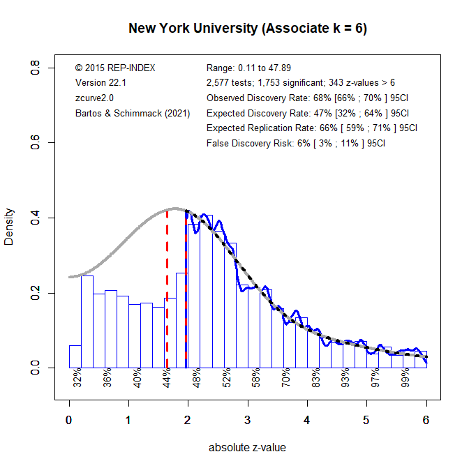
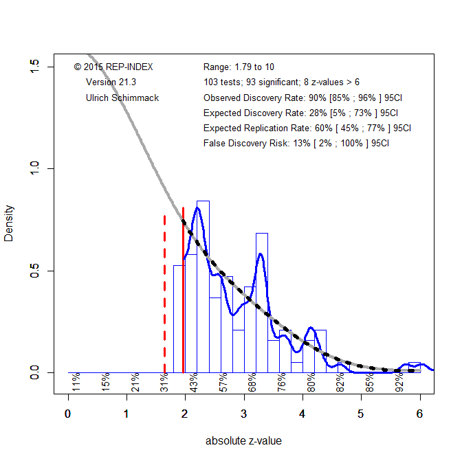
Figure 1 shows a z-curve plot for all articles from 2003-2023 (see Schimmack, 2023, for a detailed description of z-curve plots). However, the total available test statistics available for 2003, 2004 and 2005 were too low to be used individually. Therefore, these years were joined to ensure the plot had enough test statistics for each year. The plot is essentially a histogram of all test statistics converted into absolute z-scores (i.e., the direction of an effect is ignored). Z-scores can be interpreted as the strength of evidence against the null hypothesis that there is no statistical relationship between two variables (i.e., the effect size is zero and the expected z-score is zero). A z-curve plot shows the standard criterion of statistical significance (alpha = .05, z = 1.96) as a vertical red dotted line.
Figure 1
Z-curve plots are limited to values less than z = 6. The reason is that values greater than 6 are so extreme that a successful replication is all but certain unless the value is a computational error or based on fraudulent data. The extreme values are still used for the computation of z-curve statistics but omitted from the plot to highlight the shape of the distribution for diagnostic z-scores in the range from 2 to 6. Using the expectation maximization (EM) algorithm, Z-curve estimates the optimal weights for seven components located at z-values of 0, 1, …. 6 to fit the observed statistically significant z-scores. The predicted distribution is shown as a blue curve. Importantly, the model is fitted to the significant z-scores, but the model predicts the distribution of non-significant results. This makes it possible to examine publication bias (i.e., selective publishing of significant results). Using the estimated distribution of non-significant and significant results, z-curve provides an estimate of the expected discovery rate (EDR); that is, the percentage of significant results that were actually obtained without selection for significance. Using Soric’s (1989) formula the EDR is used to estimate the false discovery risk; that is, the maximum number of significant results that are false positives (i.e., the null-hypothesis is true).
Selection for Significance
The extent of selection bias in a journal can be quantified by comparing the Observed Discovery Rate (ODR) of 68%, 95%CI = 67% to 70% with the Expected Discovery Rate (EDR) of 49%, 95%CI = 26%-63%. The ODR is higher than the upper limit of the confidence interval for the EDR, suggesting the presence of selection for publication. Even though the distance between the ODR and the EDR estimate is narrower than those commonly seen in other journals the present results may underestimate the severity of the problem. This is because the analysis is based on all statistical results. Selection bias is even more problematic for focal hypothesis tests and the ODR for focal tests in psychology journals is often close to 90%.
Expected Replication Rate
The Expected Replication Rate (ERR) estimates the percentage of studies that would produce a significant result again if exact replications with the same sample size were conducted. A comparison of the ERR with the outcome of actual replication studies shows that the ERR is higher than the actual replication rate (Schimmack, 2020). Several factors can explain this discrepancy, such as the difficulty of conducting exact replication studies. Thus, the ERR is an optimist estimate. A conservative estimate is the EDR. The EDR predicts replication outcomes if significance testing does not favour studies with higher power (larger effects and smaller sampling error) because statistical tricks make it just as likely that studies with low power are published. We suggest using the EDR and ERR in combination to estimate the actual replication rate.
The ERR estimate of 72%, 95%CI = 67% to 77%, suggests that the majority of results should produce a statistically significant, p < .05, result again in exact replication studies. However, the EDR of 49% implies that there is some uncertainty about the actual replication rate for studies in this journal and that the success rate can be anywhere between 49% and 72%.
False Positive Risk
The replication crisis has led to concerns that many or even most published results are false positives (i.e., the true effect size is zero). Using Soric’s formula (1989), the maximum false discovery rate can be calculated based on the EDR.
The EDR of 49% implies a False Discovery Risk (FDR) of 6%, 95%CI = 3% to 15%, but the 95%CI of the FDR allows for up to 15% false positive results. This estimate contradicts claims that most published results are false (Ioannidis, 2005).
Changes Over Time
One advantage of automatically extracted test-statistics is that the large number of test statistics makes it possible to examine changes in publication practices over time. We were particularly interested in changes in response to awareness about the replication crisis in recent years.
Z-curve plots for every publication year were calculated to examine time trends through regression analysis. Additionally, the degrees of freedom used in F-tests and t-tests were used as a metric of sample size to observe if these changed over time. Both linear and quadratic trends were considered. The quadratic term was included to observe if any changes occurred in response to the replication crisis. That is, there may have been no changes from 2000 to 2015, but increases in EDR and ERR after 2015.
Degrees of Freedom
Figure 2 shows the median and mean degrees of freedom used in F-tests and t-tests reported in Evolutionary Psychology. The mean results are highly variable due to a few studies with extremely large sample sizes. Thus, we focus on the median to examine time trends. The median degrees of freedom over time was 121.54, ranging from 75 to 373. Regression analyses of the median showed a significant linear increase by 6 degrees of freedom per year, b = 6.08, SE = 2.57, p = 0.031. However, there was no evidence that the replication crisis influenced a significant increase in sample sizes as seen by the lack of a significant non-linear trend and a small regression coefficient, b = 0.46, SE = 0.53, p = 0.400.
Figure 2
Observed and Expected Discovery Rates
Figure 3 shows the changes in the ODR and EDR estimates over time. There were no significant linear, b = -0.52 (SE = 0.26 p = 0.063) or non-linear, b = -0.02 (SE = 0.05, p = 0.765) trends observed in the ODR estimate. The regression results for the EDR estimate showed no significant linear, b = -0.66 (SE = 0.64 p = 0.317) or non-linear, b = 0.03 (SE = 0.13 p = 0.847) changes over time. These findings indicate the journal has not increased its publication of non-significant results and continues to report more significant results than one would predict based on the mean power of studies.
Expected Replicability Rates and False Discovery Risks
Figure 4 depicts the false discovery risk (FDR) and the Estimated Replication Rate (ERR). It also shows the Expected Replication Failure rate (EFR = 1 – ERR). A comparison of the EFR with the FDR provides information for the interpretation of replication failures. If the FDR is close to the EFR, many replication failures may be due to false positive results in original studies. In contrast, if the FDR is low, most replication failures will likely be false negative results in underpowered replication studies.
The ERR estimate did not show a significant linear increase over time, b = 0.36, SE = 0.24, p = 0.165. Additionally, no significant non-linear trend was observed, b = -0.03, SE = 0.05, p = 0.523. These findings suggest the increase in sample sizes did not contribute to a statistically significant increase in the power of the published results. These results suggests that replicability of results in this journal has not increased over time and that the results in Figure 1 can be applied to all years.
Figure 4
Visual inspection of Figure 4 depicts the EFR between 30% and 40% and an FDR between 0 and 10%. This suggests that more than half of replication failures are likely to be false negatives in replication studies with the same sample sizes rather than false positive results in the original studies. Studies with large sample sizes and small confidence intervals are needed to distinguish between these two alternative explanations for replication failures.
Adjusting Alpha
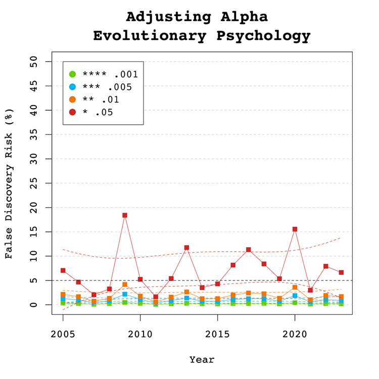
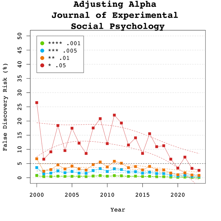
A simple solution to a crisis of confidence in published results is to adjust the criterion to reject the null-hypothesis. For example, some researchers have proposed to set alpha to .005 to avoid too many false positive results. With z-curve we can calibrate alpha to keep the false discovery risk at an acceptable level without discarding too many true positive results. To do so, we set alpha to .05, .01, .005, and .001 and examined the false discovery risk.
Figure 5
Figure 5 shows that the conventional criterion of p < .05 produces false discovery risks above 5%. The high variability in annual estimates also makes it difficult to provide precise estimates of the FDR. However, adjusting alpha to .01 is sufficient to produce an FDR with tight confidence intervals below 5%. The benefits of reducing alpha further to .005 or .001 are minimal.
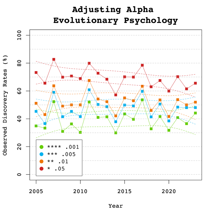
Figure 6
Figure 6 shows the impact of lowering the significance criterion, alpha, on the discovery rate (lower alpha implies fewer significant results). In Evolutionary Psychology lowering alpha to .01 reduces the observed discovery rate by about 20 to 10 percentage points. This implies that 20% of results reported p-values between .05 and .01. These results often have low success rates in actual replication studies (OSC, 2015). Thus, our recommendation is to set alpha to .01 to reduce the false positive risk to 5% and to disregard studies with weak evidence against the null-hypothesis. These studies require actual successful replications with larger samples to provide credible evidence for an evolutionary hypothesis.
There are relatively few studies with p-values between .01 and .005. Thus, more conservative researchers can use alpha = .005 without losing too many additional results.
Limitations
The main limitation of these results is the use of automatically extracted test statistics. This approach cannot distinguish between theoretically important statistical results and other results that are often reported but do not test focal hypotheses (e.g., testing the statistical significance of a manipulation check, reporting a non-significant result for a factor in a complex statistical design that was not expected to produce a significant result).
To examine the influence of automatic extraction on our results, we can compare the results to hand-coding results of over 4,000 hand-coded focal hypotheses in over 40 journals in 2010 and 2020. The ODR was 90% around 2010 and 88% around 2020. Thus, the tendency to report significant results for focal hypothesis tests is even higher than the ODR for all results and there is no indication that this bias has decreased notably over time. The ERR increased a bit from 61% to 67%, but these values are a bit lower than those reported here. Thus, it is possible that focal tests also have lower average power than other tests, but this difference seems to be small. The main finding is that the publishing of non-significant results for focal tests remains an exception in psychology journals and probably also in this journal.
One concern about the publication of our results is that it merely creates a new criterion to game publications. Rather than trying to get p-values below .05, researchers may use tricks to get p-values below .01. However, this argument ignores that it becomes increasingly harder to produce lower p-values with tricks (Simmons et al., 2011). Moreover, z-curve analysis makes it easy to see selection bias for different levels of significance. Thus, a more plausible response to these results is that researchers will increase sample sizes or use other methods to reduce sampling error to increase power.
Conclusion
The replicability report shows that the average power to report a significant result (i.e., a discovery) ranges from 49% to 72% in Evolutionary Psychology. This finding is higher than previous estimates observed in evolutionary psychology journals. However, the confidence intervals are wide and suggest that many published studies remain underpowered. The report did not capture any significant changes over time in the power and replicability as captured by the EDR and the ERR estimates. The false positive risk is modest and can be controlled by setting alpha to .01. Replication attempts of original findings with p-values above .01 should increase sample sizes to produce more conclusive evidence. Lastly, the journal shows clear evidence of selection bias.
There are several ways, the current or future editors of this journal can improve the credibility of results published in this journal. First, results with weak evidence (p-values between .05 and .01) should only be reported as suggestive results that require replication or even request a replication before publication. Second, editors should try to reduce publication bias by prioritizing research questions over results. A well-conducted study with an important question should be published even if the results are not statistically significant. Pre-registration and registered reports can help to reduce publication bias. Editors may also ask for follow-up studies with higher power to follow up on a non-significant result.
Publication bias also implies that point estimates of effect sizes are inflated. It is therefore important to take uncertainty in these estimates into account. Small samples with large sampling errors are usually unable to provide meaningful information about effect sizes and conclusions should be limited to the direction of an effect.
The present results serve as a benchmark for future years to track progress in this journal to ensure trust in research by evolutionary psychologists.
Citation: Soto, M. & Schimmack, U. (2024, July 4/08/13).  2024 Replicability Report for the Journal of Experimental Social Psychology.  Replicability Index.
https://replicationindex.com/2024/07/04/rr24-jesp/
Introduction
In the 2010s, it became apparent that empirical psychology had a replication problem. When psychologists tested the replicability of 100 results, they found that only 36% of the 97 significant results in original studies could be reproduced (Open Science Collaboration, 2015). In addition, several prominent cases of research fraud further undermined trust in published results. Over the past decade, several proposals were made to improve the credibility of psychology as a science. Replicability Reports aim to improve the credibility of psychological science by examining the amount of publication bias and the strength of evidence for empirical claims in psychology journals.
The main problem in psychological science is the selective publishing of statistically significant results and the blind trust in statistically significant results as evidence for researchers’ theoretical claims. Unfortunately, psychologists have been unable to self-regulate their behaviour and continue to use unscientific practices to hide evidence that disconfirms their predictions. Moreover, ethical researchers who do not use unscientific practices are at a disadvantage in a game that rewards publishing many articles without concern about these findings’ replicability. Replicability reports aim to reward journals that publish credible results and use open science practices that encourage honest reporting of results like preregistration or registered reports.
My colleagues and I have developed a statistical tools that can reveal the use of unscientific practices and predict the outcome of replication studies (Brunner & Schimmack, 2021; Bartos & Schimmack, 2022). This method is called z-curve. Z-curve cannot be used to evaluate the credibility of a single study. However, it can provide valuable information about the research practices in a particular research domain. Replicability-Reports (RR) analyze the statistical results reported in a journal with z-curve to estimate the replicability of published results, the amount of publication bias, and the risk that significant results are false positive results (i.e, the sign of a mean difference or correlation of a significant result does not match the sign in the population).
Journal of Experimental Social Psychology
The Journal of Experimental Social Psychology (JESP) was established in 1965. It is the oldest journal that specializes on experimental studies of social cognitions and behaviors. A replicability analysis of this journal is particularly interesting for several reasons. First, the long history of the journal makes it possible to examine historic trends in research practices in this field over a long time period. Second, experimental social psychology has triggered the crisis of confidence in psychological science with studies on extrasensory perception (Bem, 2011), implicit priming (Bargh et al., 1996), and ego depletion (Baumeister et al., 1996) that failed to replicate. At the same time, social psychology has responded to these replication failures by increasing sample sizes and rewarding open science practices like preregistration of analyses plans that limit researchers’ degrees of freedom to fish for significance or change hypotheses after examining the data.
On average, JESP publishes about 150 articles in 6 annual issues. According to Web of Science, the impact factor of JESP ranks 15th in the Psychology, Social category (Clarivate, 2024). The journal has an H-Index of 196 (i.e., 196 articles have received 196 or more citations).
In its lifetime, Journal of Experimental Social Psychology (JESP) has published over 4,200 articles with an average citation rate of 56.01 citations. So far, the journal has published 10 articles with more than 1,000 citations. Most of these have been published before the 2000s. The three most cited articles in the 2000s focus on improving methods used in social psychology research (Oppenheimer et al., 2009; Leys et al., 2013; Peer et al., 2017).
The Open Science Collaboration observed how only 14 out of 55 (25%) social psychology effects were replicated. A similar replicability estimate of 16% to 44% was measured for social psychology by Bartoš & Schimmack (2022). In response, many journals have implemented multiple strategies to improve the replicability and credibility of their published findings. Similarly, JESP introduced the “JESP’s 10-Item Submission Checklist” in 2022. The list entails a series of requirements that authors must fulfill to have their manuscripts reviewed. This checklist requires that authors provide their priori power analysis, sample size determination, and full reporting of all statistics including non-significant ones, among other items that aim to improve the quality of the submitted manuscripts. JESP’s focus on social psychology allows this report to highlight whether the proposed strategies to reform social psychology research meet their expectations.
The current Editor-in-Chief is Professor Nicholas Rule. Professor Kristin Laurin serves as the Senior Associate Editor. The associate editors are Professor Rachel Barkan, Professor Pamela K Smith, Professor Fiona Barlow, Professor Paul Conway, Professor Jarret Crawford, Professor Sarah Gaither, Professor Shlomo Hareli, Professor Edward Hirt, Professor Rachael Jack, Professor Joris Lammers, Professor Pranjal H. Mehta, Professor Kristin Pauker, Professor Brett Peters, Professor Evava Pietr, and Professor Karina Schumann.
Extraction Method
Replication reports are based on automatically extracted test statistics such as F-tests, t-tests, z-tests, and chi2-tests. Additionally, we extracted 95% confidence intervals of odds ratios and regression coefficients. The test statistics were extracted from collected PDF files using a custom R-code. The code relies on the pdftools R package (Ooms, 2024) to render all textboxes from a PDF file into character strings. Once converted the code proceeds to systematically extract the test statistics of interest (Soto & Schimmack, 2024). PDF files identified as editorials, review papers and meta-analyses were excluded. Meta-analyses were excluded to avoid the inclusion of test statistics that were not originally published in the Journal of Experimental Social Psychology. Following extraction, the test statistics are converted into absolute z-scores.
Results For All Years
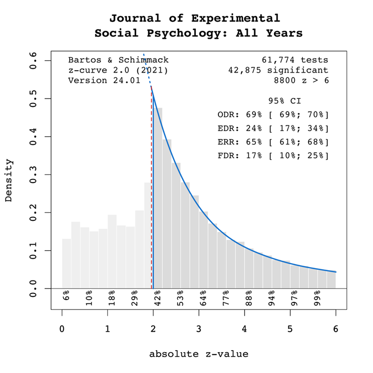
Figure 1 shows a z-curve plot for all articles from 2000-2023 (see Schimmack, 2023, for a detailed description of z-curve plots). The plot is essentially a histogram of all test statistics converted into absolute z-scores (i.e., the direction of an effect is ignored). Z-scores can be interpreted as the strength of evidence against the null hypothesis that there is no statistical relationship between two variables (i.e., the effect size is zero and the expected z-score is zero). A z-curve plot shows the standard criterion of statistical significance (alpha = .05, z = 1.96) as a vertical red dotted line.
Figure 1
Z-curve plots are limited to values less than z = 6. The reason is that values greater than 6 are so extreme that a successful replication is all but certain unless the value is a computational error or based on fraudulent data. The extreme values are still used for the computation of z-curve statistics but omitted from the plot to highlight the shape of the distribution for diagnostic z-scores in the range from 2 to 6. Using the expectation maximization (EM) algorithm, Z-curve estimates the optimal weights for seven components located at z-values of 0, 1, …. 6 to fit the observed statistically significant z-scores. The predicted distribution is shown as a blue curve. Importantly, the model is fitted to the significant z-scores, but the model predicts the distribution of non-significant results. This makes it possible to examine publication bias (i.e., selective publishing of significant results). Using the estimated distribution of non-significant and significant results, z-curve provides an estimate of the expected discovery rate (EDR); that is, the percentage of significant results that were actually obtained without selection for significance. Using Soric’s (1989) formula the EDR is used to estimate the false discovery risk; that is, the maximum number of significant results that are false positives (i.e., the null-hypothesis is true).
Selection for Significance
The extent of selection bias in a journal can be quantified by comparing the Observed Discovery Rate (ODR) of 69%, 95%CI = 69% to 70% with the Expected Discovery Rate (EDR) of 24%, 95%CI = 17%-34%. The ODR is notably higher than the upper confidence interval limit for the EDR, indicating statistically significant publication bias. Furthermore, there is clear evidence of selection for significance given that the ODR estimate is more than double the point estimate of the EDR.
It is also noteworthy that the present results probably underestimate severity of selection bias for focal hypothesis test. The present results do no distinguish between theoretically important and complementary analyses. It is known that focal hypothesis tests in psychology before the replication crisis have an observed success rate over 90% (Sterling, 1959; Sterling et al., 1995; Motyl et al., 2017). While it is possible that focal tests also have higher power, it is likely that the differences in the ODR larger than the differences in the EDR.
In conclusion, the present results are consistent with the finding that replication studies are more likely to produce non-significant results than reported original findings because selection for significance inflates the percentage of significant results in published articles (OSC, 2015).
Expected Replication Rate
The Expected Replication Rate (ERR) estimates the percentage of studies that would produce a significant result again if exact replications with the same sample size were conducted. A comparison of the ERR with the outcome of actual replication studies shows that the ERR is higher than the actual replication rate (Schimmack, 2020). Several factors can explain this discrepancy, including the difficulty of conducting exact replication studies. Thus, the ERR is an optimist estimate. A conservative estimate is the EDR. The EDR predicts replication outcomes if significance testing does not favour studies with higher power (larger effects and smaller sampling error) because statistical tricks make it just as likely that studies with low power are published. We suggest using the EDR and ERR in combination to estimate the actual replication rate.
The Expected Replication Rate (ERR) estimates the percentage of studies that would produce a significant result again if exact replications with the same sample size were conducted. A comparison of the ERR with the outcome of actual replication studies shows that the ERR is higher than the actual replication rate (Schimmack, 2020). Several factors can explain this discrepancy, such as the difficulty of conducting exact replication studies. Thus, the ERR is an optimist estimate. A conservative estimate is the EDR. The EDR predicts replication outcomes if significance testing does not favour studies with higher power (larger effects and smaller sampling error) because statistical tricks make it just as likely that studies with low power are published. We suggest using the EDR and ERR in combination to estimate the actual replication rate.
The ERR estimate of 65%, 95%CI = 61% to 68%, suggests that most results should produce a statistically significant, p < .05, result again in exact replication studies. However, the EDR of 24% implies considerable uncertainty about the actual replication rate for studies in this journal and that the success rate can be between 24% and 65%. These estimates can be compared with the actual success rate of replications of social psychological experiments in the Reproducibility Project of 25% (OSC, 2015). While this estimate is based on a small, unrepresentative sample, it does confirm that the replication rate of social psychological experiments can be as low as 1 out of 4 studies. This justifies concerns about the credibility of results published in JESP (see also Schimmack, 2020).
False Positive Risk
The replication crisis has led to concerns that many or even most published results are false positives (i.e., the true effect size is zero or in the opposite direction). The high rate of replication failures, however, may simply reflect low power to produce significant results for true positives and does not tell us how many published results are false positives. We can provide some information about the false positive risk based on the EDR. Using Soric’s formula (1989), the EDR can be used to calculate the maximum false discovery rate.
The EDR of 24% implies a False Discovery Risk (FDR) of 17%, 95%CI = 10% to 25%, but the 95%CI of the FDR allows for up to 25% false positive results. This estimate contradicts claims that most published results are false (Ioannidis, 2005), but the results also create uncertainty about the credibility of results with statistically significant results, if up to 1 out of 4 results can be false positives. For readers it may be difficult to decide whether a published results can be trusted.
Time Trends
One advantage of automatically extracted test-statistics is that the large number of test statistics makes it possible to examine changes in publication practices over time. We were particularly interested in changes in response to awareness about the replication crisis in recent years.
Z-curve plots for every publication year were calculated to examine time trends through regression analysis. Additionally, the degrees of freedom used in F-tests and t-tests were used as a metric of sample size to observe if these changed over time. Both linear and quadratic trends were considered. The quadratic term was included to observe if any changes occurred in response to the replication crisis. That is, there may have been no changes from 2000 to 2015, but increases in EDR and ERR after 2015.
Degrees of Freedom
Figure 2 shows the median and mean degrees of freedom used in F-tests and t-tests reported in the Journal of Experimental Social Psychology. The mean results are highly variable due to a few studies with extremely large sample sizes. Thus, we focus on the median to examine time trends. The median degree of freedom over time was 82.25, ranging from 60 to 302. Regression analyses of the median showed a significant linear increase by about 9 degrees of freedom per year, b = 9.13, SE = 0.62, p < 0.0001. Furthermore, there was a statistically significant non-linear increase, b = 0.94, SE = 0.10, p < 0.0001, suggesting that the replication crisis led to an increase in sample sizes. As larger samples increase power, we would expect an increase in the ERR and EDR.
Figure 2
Observed and Expected Discovery Rates
Figure 3 shows the changes in the ODR and EDR estimates over time. There was a significant linear decrease to the ODR estimate by 0.44 percentage points per year, b = -0.44, SE = 0.08, p < 0.0001. No significant non-linear, b = 0.01 (SE = 0.01, p = 0.27) trend was observed in the ODR estimate. These results show that researchers have published more non-significant results over time, leading to a decrease in selection bias.
The regression results for the EDR estimate showed significant linear, b = 1.14 (SE = 0.25 p < 0.001) and non-linear, b = 0.17 (SE = 0.04 p < 0.001) changes over time. The non-linear trend is consistent with the results for the degrees of freedom and confirms that power has increased after the replication crisis due to the use of larger samples. This also reduces selection bias. The trends for the ODR and EDR have narrowed the gap between the ODR and the EDR as seen in Figure 3. However, it remains to be seen whether this trend also applies to focal hypothesis tests.
Figure 3
Expected Replicability Rates and False Discovery Risks
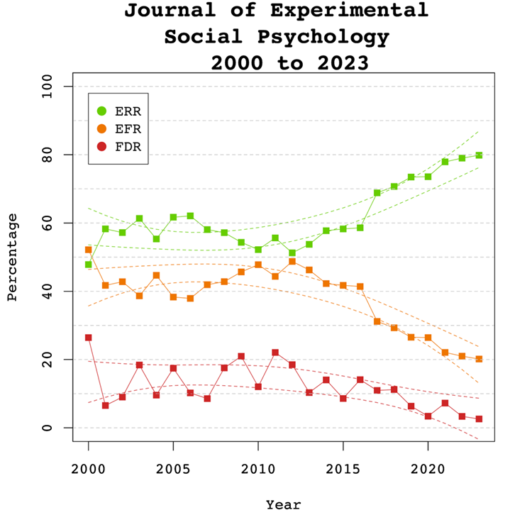
Figure 4 depicts the false discovery risk (FDR) and the Estimated Replication Rate (ERR). It also shows the Expected Replication Failure rate (EFR = 1 – ERR). A comparison of the EFR with the FDR provides information for the interpretation of replication failures. If the FDR is close to the EFR, many replication failures may be due to false positive results in original studies. In contrast, if the FDR is low, most replication failures will likely be false negative results in underpowered replication studies.
There were no significant linear, b = 0.13, SE = 0.10, p = 0.204 or non-linear, b = 0.01, SE = 0.16, p = 0.392 trends observed in the ERR estimate. These findings are inconsistent with the observed significant increase in sample sizes as the reduction in sampling error often increases the likelihood that an effect will replicate. One possible explanation for this is that the type of studies has changed. If a journal publishes more studies from disciplines with large samples and small effect sizes, sample sizes go up without increasing power. Thus, analysis of sample size alone provide insufficient information about the credibility of published results.
Visual inspection of Figure 4 depicts the EFR consistently around 30% and the FDR around 10%, suggesting that about one-third of replication failures are false positive results in original studies. The larger decrease for the EFR than the FDR suggests that larger samples have mainly reduced false negative results and increasing the probability that a replication failure reveals a false positive result in the original study.
Figure 4
Adjusting Alpha
A simple solution to a crisis of confidence in published results is to adjust the criterion to reject the null-hypothesis. For example, some researchers have proposed to set alpha to .005 to avoid too many false positive results. With z-curve we can calibrate alpha to keep the false discovery risk at an acceptable level without discarding too many true positive results. To do so, we set alpha to .05, .01, .005, and .001 and examined the false discovery risk.
Figure 5
Figure 5 shows that the conventional criterion of p < .05 produces false discovery risks above 5%. The high variability in annual estimates also makes it difficult to provide precise estimates of the FDR. However, adjusting alpha to .01 is sufficient to produce an FDR with tight confidence intervals below 5%. More conservative readers might adjust to p < 0.005 for results published between 2007 and 2013. Overall, the benefits of reducing alpha further to .005 or .001 are minimal.
Figure 6
Figure 6 shows the impact of lowering the significance criterion, alpha, on the discovery rate (lower alpha implies fewer significant results). In the Journal of Experimental Social Psychology lowering alpha to .01 reduces the observed discovery rate considerably in the years before the replication crisis from about 70-80% to just 40-50% of reported results. The reason is that statistical tricks are more likely to produce just significant results between .05 and .01 than lower p-values (Simmons et al., 2011). Therese results are also much less likely to replicate (OSC, 2015). Thus, it is reasonable to treat these results as not significant and to require a credible replication study. In recent years, more p-values are below .01 and using alpha = .01 as significance criterion has relatively little impact on the discovery rate. Lowering alpha further has relatively little effect on the discovery rate. While these results should not be interpreted as a call for official changes to the alpha criterion, they help readers to evaluate the costs and benefits of using a specific alpha level. We believe that alpha = .01 provides an optimal trade-off for results published in JESP.
Limitations
One concern about the publication of our results is that it merely creates a new criterion to game publications. Rather than trying to get p-values below .05, researchers may use tricks to get p-values below .01. However, this argument ignores that it becomes increasingly harder to produce lower p-values with tricks (Simmons et al., 2011). Moreover, z-curve analysis makes it easy to see selection bias for different levels of significance. Thus, a more plausible response to these results is that researchers will increase sample sizes or use other methods to reduce sampling error to increase power. Our trend analyses show that this has already happened and that results published after 2015 are more credible.
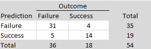
A bigger concern is that our results underestimate the severity of the problem because they do not distinguish between theoretically important (focal) and additional (non-focal) hypothesis tests. To address this concern it is necessary to identify focal hypothesis tests and to hand-code results of these tests. For JESP, we were able to use hand-coded data from Motyl et al.’s (2017) article that randomly selected focal hypothesis tests from several journals, including JESP. The data are based on the years 2003, 2004, 2013, and 2014 and are representative for the years before reforms increased replicability (see Figures 3 & 4).
Figure 7
The ODR is similar to the ODR for all test statistics (70% vs. 69%, but non-significant results are clustered just below the significance level of .05 and are often used to reject the null-hypothesis with “marginal significance” (p < .10, z > 1.65). If these results are counted as ‘significant’, the ODR is 87%, which is close to Sterling et al.’s (1995) findings that over 90% of hypothesis tests in psychology reject the null-hypothesis. In contrast, the estimate of the expected discovery rate is only 14%, which is lower than the estimate for all hypothesis tests (Figure 1, 24%). Although the small number of studies leads to wide confidence intervals, the results suggest that focal tests have even lower power than other tests. The confidence interval for the EDR even includes 5%, which would imply that power equals alpha, which is the case when the population effect sizes are zero. This also implies that the confidence interval for the FDR includes 100%, suggesting that all focal hypothesis are false. Of course, it is unlikely that social psychologists only reported false results for decades, but the evidence is so weak that it is impossible to know which of these results are true and which ones are false. In this case, adjusting alpha does not help because the upper limit of the FDR confidence interval remains at 100% because the lower bound of the confidence interval for the EDR remains at 5%. Until more evidence for focal tests is obtained, it may be justified to use the results for all tests, but the false discovery risk for focal tests with p-values below .01 may be higher than 5%. Given so much uncertainty about results published in JESP before 2015, single studies should not be interpreted and important studies should be replicated with larger samples and preregistration.
Conclusion
The replicability report for the Journal of Experimental Social Psychology suggests that the power to obtain a significant result to report a significant result (i.e., a discovery) ranges from 24% to 65%, and may be even lower for focal hypothesis tests. This finding suggests that many studies are underpowered and require luck to get a significant result. The false positive risk is considerable but can be controlled by setting alpha to .01 during most years. However, an analysis of a small set of focal tests suggests that this criterion is too liberal for focal tests, but it is impossible to quantify the false discovery risk for focal tests.
Our results show clear evidence of improvement in response to the replication crisis. Power has increased with the help of larger samples and selection bias has decreased. This is a welcome development. It also means that our recommendation to use alpha of .01 penalizes only a smaller set of studies with p-values between .05 and .01. Of course, these results can occur by chance and can be false negatives, but in this case researchers should conduct additional studies to strengthen evidence for their hypothesis.
Hand-coding of focal tests after 2015 would provide important information about the credibility of focal tests in recent years. One important question is whether the journal publishes studies with non-significant results in large samples that suggest a hypothesis was false. These results would best be reported with 95%CI that limit plausible effect sizes to values close to zero. After all, risky hypotheses are bound to be false sometimes.
In conclusion, our results provide some valuable empirical evidence about the credibility of results published in JESP. The main finding is that results before the replication crisis had low credibility and were often obtained by selectively reporting confirmatory evidence. This has changed and results in recent years have much less selection bias and are more credible.
In the 2010s, it became apparent that empirical psychology had a replication problem. When psychologists tested the replicability of 100 results, they found that only 36% of the 97 significant results in original studies could be reproduced (Open Science Collaboration, 2015). In addition, several prominent cases of research fraud further undermined trust in published results. Over the past decade, several proposals were made to improve the credibility of psychology as a science. Replicability Reports aim to improve the credibility of psychological science by examining the amount of publication bias and the strength of evidence for empirical claims in psychology journals.
The main problem in psychological science is the selective publishing of statistically significant results and the blind trust in statistically significant results as evidence for researchers’ theoretical claims. Unfortunately, psychologists have been unable to self-regulate their behavior and continue to use unscientific practices to hide evidence that disconfirms their predictions. Moreover, ethical researchers who do not use unscientific practices are at a disadvantage in a game that rewards publishing many articles without any concern about the replicability of these findings.
My colleagues and I have developed a statistical tools that can reveal the use of unscientific practices and predict the outcome of replication studies (Brunner & Schimmack, 2021; Bartos & Schimmack, 2022). This method is called z-curve. Z-curve cannot be used to evaluate the credibility of a single study. However, it can provide valuable information about the research practices in a particular research domain. Replicability-Reports (RR) analyze the statistical results reported in a journal with z-curve to estimate the replicability of published results, the amount of publication bias, and the risk that significant results are false positive results (i.e, the sign of a mean difference or correlation of a significant result does not match the sign in the population).
Acta Psychologica
Acta Psychologica is an old psychological journal that was founded in 1936. The journal publishes articles from various areas of psychology, but cognitive psychological research seems to be the most common area. Since 2021, the journal is a Gold Open Access journal that charges authors a $2,000 publication fee.
On average, Acta Psychologica publishes about 150 articles a year in 9 annual issues.
According to Web of Science, the impact factor of Acta Psychologica ranks 44th in the Experimental Psychology category (Clarivate, 2024). The journal has an H-Index of 140 (i.e., 140 articles have received 140 or more citations).
In its lifetime, Acta Psychologica has published over 6,000 articles with an average citation rate of 21.5 citations. So far, the journal has published 5 articles with more than 1,000 citations. However, most of these articles were published in the 1960s and 1970s. The most highly cited article published in the 2000s examined the influence of response categories on the psychometric properties of survey items (Preston & Colman, 2000; 1055 citations).
Psychology literature has faced difficult realizations in the last decade. Acta Psychologica is a broad-scope journal that offers us the possibility to observe changes in the robustness of psychological research practices and results. The current report serves as a glimpse into overall trends in psychology literature as it considers research from multiple subfields.
Given the multidisciplinary nature of the journal, the journal has a team of editors. The current editors are Dr. Muhammad Abbas, Dr. Mohamed Alansari, Dr. Colin Cooper, Dr. Valerie De Cristofaro, Dr. Nerelie Freeman, Professor, Alessandro Gabbiadini, Professor Matthieu Guitton, Dr. Nhung T Hendy, Dr. Amanpreet Kaur, Dr. Shengjie Lin, Dr. Hui Jing Lu, Professor Robrecht Van Der Wel and Dr. Olvier Weigelt.
Extraction Method
Replication reports are based on automatically extracted test statistics such as F-tests, t-tests, z-tests, and chi2-tests. Additionally, we extracted 95% confidence intervals of odds ratios and regression coefficients. The test statistics were extracted from collected PDF files using a custom R-code. The code relies on the pdftools R package (Ooms, 2024) to render all textboxes from a PDF file into character strings. Once converted the code proceeds to systematically extract the test statistics of interest (Soto & Schimmack, 2024). PDF files identified as editorials, review papers and meta-analyses were excluded. Meta-analyses were excluded to avoid the inclusion of test statistics that were not originally published in Acta Psychologica Following extraction, the test statistics are converted into absolute z-scores.
Results For All Years
Figure 1 shows a z-curve plot for all articles from 2000-2023 (see Schimmack, 2022a, 2022b, for a detailed description of z-curve plots). The plot is essentially a histogram of all test statistics converted into absolute z-scores (i.e., the direction of an effect is ignored). Z-scores can be interpreted as the strength of evidence against the null hypothesis that there is no statistical relationship between two variables (i.e., the effect size is zero and the expected z-score is zero). A z-curve plot shows the standard criterion of statistical significance (alpha = .05, z = 1.96) as a vertical red dotted line.
Figure 1
Z-curve plots are limited to values less than z = 6. The reason is that values greater than 6 are so extreme that a successful replication is all but certain unless the value is a computational error or based on fraudulent data. The extreme values are still used for the computation of z-curve statistics but omitted from the plot to highlight the shape of the distribution for diagnostic z-scores in the range from 2 to 6. Using the expectation maximization (EM) algorithm, Z-curve estimates the optimal weights for seven components located at z-values of 0, 1, …. 6 to fit the observed statistically significant z-scores. The predicted distribution is shown as a blue curve. Importantly, the model is fitted to the significant z-scores, but the model predicts the distribution of non-significant results. This makes it possible to examine publication bias (i.e., selective publishing of significant results). Using the estimated distribution of non-significant and significant results, z-curve provides an estimate of the expected discovery rate (EDR); that is, the percentage of significant results that were actually obtained without selection for significance. Using Soric’s (1989) formula the EDR is used to estimate the false discovery risk; that is, the maximum number of significant results that are false positives (i.e., the null-hypothesis is true).
Selection for Significance
The extent of selection bias in a journal can be quantified by comparing the Observed Discovery Rate (ODR) of 70%, 95%CI = 70% to 71% with the Expected Discovery Rate (EDR) of 38%, 95%CI = 27%-54%. The ODR is notably higher than the upper limit of the confidence interval for the EDR, indicating statistically significant publication bias. It is noteworthy that the present results may underestimate the severity of the problem because the analysis is based on all statistical results. Selection bias is even more problematic for focal hypothesis tests and the ODR for focal tests in psychology journals is often higher than the ODR for all tests. Thus, the current results are a conservative estimate of bias for critical hypothesis tests.
Expected Replication Rate
The Expected Replication Rate (ERR) estimates the percentage of studies that would produce a significant result again if exact replications with the same sample size were conducted. A comparison of the ERR with the outcome of actual replication studies shows that the ERR is higher than the actual replication rate (Schimmack, 2020). Several factors can explain this discrepancy, including the difficulty of conducting exact replication studies. Thus, the ERR is an optimist estimate. A conservative estimate is the EDR. The EDR predicts replication outcomes if significance testing does not favour studies with higher power (larger effects and smaller sampling error) because statistical tricks make it just as likely that studies with low power are published. We suggest using the EDR and ERR in combination to estimate the actual replication rate.
The ERR estimate of 73%, 95%CI = 69% to 77%, suggests that the majority of results should produce a statistically significant, p < .05, result again in exact replication studies. However, the EDR of 38% implies that there is considerable uncertainty about the actual replication rate for studies in this journal and that the success rate can be anywhere between 27% and 77%.
False Positive Risk
The replication crisis has led to concerns that many or even most published results are false positives (i.e., the true effect size is zero or in the opposite direction). The high rate of replication failures, however, may simply reflect low power to produce significant results for true positives and does not tell us how many published results are false positives. We can provide some information about the false positive risk based on the EDR. Using Soric’s formula (1989), the EDR can be used to calculate the maximum false discovery rate.
The EDR of 38% for Acta Psychologica implies a False Discovery Risk (FDR) of 9%, 95%CI = 5% to 15%, but the 95%CI of the FDR allows for up to 15% false positive results. This estimate contradicts claims that most published results are false (Ioannidis, 2005), but is probably a bit higher than many readers of this journal would like.
Time Trends
One advantage of automatically extracted test-statistics is that the large number of test statistics makes it possible to examine changes in publication practices over time. We were particularly interested in changes in response to awareness about the replication crisis in recent years.
Z-curve plots for every publication year were calculated to examine time trends through regression analysis. Additionally, the degrees of freedom used in F-tests and t-tests were used as a metric of sample size to observe if these changed over time. Both linear and quadratic trends were considered. The quadratic term was included to observe if any changes occurred in response to the replication crisis. That is, there may have been no changes from 2000 to 2015 but increases in EDR and ERR after 2015.
Degrees of Freedom
Figure 2 shows the median and mean degrees of freedom used in F-tests and t-tests reported in Acta Psychologica. The mean results are highly variable due to a few studies with extremely large sample sizes. Thus, we focus on the median to examine time trends. The median degrees of freedom over time was 38, ranging from 22 to 74. Regression analyses of the median showed a significant linear increase of a 1.4 degrees of freedom per year, b = 1.39, SE = 3.00, p < 0.0001. Furthermore, the results suggest the replication crisis influenced a significant increase in sample sizes noted by the significant non-linear trend, b = 0.09, SE = 0.03, p = 0.007.
Figure 2
Observed and Expected Discovery Rates
Figure 3 shows the changes in the ODR and EDR estimates over time. The ODR estimate showed a significant linear decrease of about b = -0.42 (SE = 0.10 p = 0.001) percentage points per year. The results did not show a significant non-linear trend in the ODR estimate, b = -0.10 (SE = 0.02, p = 0.563. The regression results for the EDR estimate showed no significant trends, linear, b = 0.04, SE = 0.37, p = 0.903, non-linear, b = 0.01, SE = 0.06, p = 0.906.
These findings indicate the journal has increased the publication of non-significant results. However, there is no evidence that this change occurred in response to the replicability crisis. Even with this change, the ODR and EDR estimates do not overlap, indicating that selection bias is still present. Furthermore, the lack of changes to the EDR suggests that many studies continue to be statistically underpowered to detect true effects.
Figure 3
Expected Replicability Rates and False Discovery Risks
Figure 4 depicts the false discovery risk (FDR) and the Estimated Replication Rate (ERR). It also shows the Expected Replication Failure rate (EFR = 1 – ERR). A comparison of the EFR with the FDR provides information for the interpretation of replication failures. If the FDR is close to the EFR, many replication failures may be due to false positive results in original studies. In contrast, if the FDR is low, most replication failures will likely be false negative results in underpowered replication studies.
There were no significant linear, b = 0.13, SE = 0.10, p = 0.204 or non-linear, b = 0.01, SE = 0.16, p = 0.392 trends observed in the ERR estimate. These findings are inconsistent with the observed significant increase in sample sizes as the reduction in sampling error often increases the likelihood that an effect will replicate. One possible explanation for this is that the type of studies has changed. If a journal publishes more studies from disciplines with large samples and small effect sizes, sample sizes go up without increasing power.
Given the lack of change in the EDR and ERR estimate over time, many published significant results are based on underpowered studies that are difficult to replicate.
Figure 4
Visual inspection of Figure 4 depicts the EFR consistently around 30% and the FDR around 10%, suggesting that about 30% of replication failures are false positives.
Adjusting Alpha
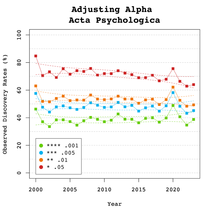
A simple solution to a crisis of confidence in published results is to adjust the criterion to reject the null-hypothesis. For example, some researchers have proposed to set alpha to .005 to avoid too many false positive results. With z-curve, we can calibrate alpha to keep the false discovery risk at an acceptable level without discarding too many true positive results. To do so, we set alpha to .05, .01, .005, and .001 and examined the false discovery risk.
Figure 5
Figure 5 shows that the conventional criterion of p < .05 produces false discovery risks above 5%. The high variability in annual estimates also makes it difficult to provide precise estimates of the FDR. However, adjusting alpha to .01 is sufficient to produce an FDR with tight confidence intervals below 5%. The benefits of reducing alpha further to .005 or .001 are minimal.
Figure 6
Figure 6 shows the impact of lowering the significance criterion, alpha, on the discovery rate (lower alpha implies fewer significant results). In Acta Psychologica lowering alpha to .01 reduces the observed discovery rate by about 20 percentage points. This implies that 20% of results reported p-values between .05 and .01. These results often have low success rates in actual replication studies (OSC, 2015). Thus, our recommendation is to set alpha to .01 to reduce the false positive risk to 5% and to disregard studies with weak evidence against the null-hypothesis. These studies require actual successful replications with larger samples to provide credible evidence for an evolutionary hypothesis. There are relatively few studies with p-values between .01 and .005. Thus, more conservative researchers can use alpha = .005 without losing too many additional results.
Limitations
The main limitation of these results is the use of automatically extracted test statistics. This approach cannot distinguish between theoretically important statistical results and other results that are often reported but do not test focal hypotheses (e.g., testing the statistical significance of a manipulation check, reporting a non-significant result for a factor in a complex statistical design that was not expected to produce a significant result).
Hand-coding of 81 studies in 2010 and 112 studies from 2020 showed ODRs of 98%, 95%CI = 94%-100% and 91%, 95%CI = 86%-96%, suggesting a slight increase in reporting of non-significant focal tests. However, ODRs over 90% suggest that publication bias is still present in this journal. ERR estimates were similar and the small sample size made it impossible to obtain reliable estimates of the EDR and FDR.
One concern about the publication of our results is that it merely creates a new criterion to game publications. Rather than trying to get p-values below .05, researchers may use tricks to get p-values below .01. However, this argument ignores that it becomes increasingly harder to produce lower p-values with tricks (Simmons et al., 2011). Moreover, z-curve analysis makes it easy to see selection bias for different levels of significance. Thus, a more plausible response to these results is that researchers will increase sample sizes or use other methods to reduce sampling error to increase power.
Conclusion
The replicability report for Acta Psychologica shows clear evidence of selection bias, although there is a trend that selection bias has decreased due to reporting of more non-significant results, but not necessarily focal ones. The power to obtain a significant result to report a significant result (i.e., a discovery) ranges from 38% to 73%. This finding suggests that many studies are underpowered and require luck to get a significant result. The false positive risk is modest and can be controlled by setting alpha to .01. Replication attempts of original findings with p-values above .01 should increase sample sizes to produce more conclusive evidence.
There are several ways, the current or future editors of this journal can improve credibility of results published in this journal. First, results with weak evidence (p-values between .05 and .01) should only be reported as suggestive results that require replication or even request a replication before publication. Second, editors should try to reduce publication bias by prioritizing research questions over results. A well-conducted study with an important question should be published even if the results are not statistically significant. Pre-registration and registered reports can help to reduce publication bias. Editors may also ask for follow-up studies with higher power to follow up on a non-significant result.
Publication bias also implies that point estimates of effect sizes are inflated. It is therefore important to take uncertainty in these estimates into account. Small samples with large sampling errors are usually unable to provide meaningful information about effect sizes and conclusions should be limited to the direction of an effect.
We hope that these results provide readers of this journal with useful informatoin to evaluate the credibility of results reported in this journal. The results also provide a benchmark to evaluate the influence of reforms on the credibility of psychological science. We hope that reform initiatives will increase power and decrease publication bias and false positive risks.
In the 2010s, it became apparent that empirical psychology had a replication problem. When psychologists tested the replicability of 100 results, they found that only 36% of the 97 significant results in original studies could be reproduced (Open Science Collaboration, 2015). In addition, several prominent cases of research fraud further undermined trust in published results. Over the past decade, several proposals were made to improve the credibility of psychology as a science. Replicability Reports aim to improve the credibilty of psychological science by examining the amount of publication bias and the strength of evidence for empirical claims in psychology journals.
The main problem in psychological science is the selective publishing of statistically significant results and the blind trust in statistically significant results as evidence for researchers’ theoretical claims. Unfortunately, psychologists have been unable to self-regulate their behaviour and continue to use unscientific practices to hide evidence that disconfirms their predictions. Moreover, ethical researchers who do not use unscientific practices are at a disadvantage in a game that rewards publishing many articles without concern about these findings’ replicability.
My colleagues and I have developed a statistical tool that can reveal the use of unscientific practices and predict the outcome of replication studies (Brunner & Schimmack, 2021; Bartos & Schimmack, 2022). This method is called z-curve. Z-curve cannot be used to evaluate the credibility of a single study. However, it can provide valuable information about the research practices in a particular research domain.
Replicability-Reports (RR) use z-curve to provide information about psychological journal research and publication practices. This information can aid authors choose journals they want to publish in, provide feedback to journal editors who influence selection bias and replicability of published results, and, most importantly, to readers of these journals.
Evolution & Human Behavior
Evolution & Human Behavior is the official journal of the Human Behaviour and Evolution Society. It is an interdisciplinary journal founded in 1997. The journal publishes articles on human behaviour from an evolutionary perspective. On average, Evolution & Human Behavior publishes about 70 articles a year in 6 annual issues.
Evolutionary psychology has produced both highly robust and questionable results. Robust results have been found for sex differences in behaviors and attitudes related to sexuality. Questionable results have been reported for changes in women’s attitudes and behaviors as a function of hormonal changes throughout their menstrual cycle.
According to Web of Science, the impact factor of Evolution & Human Behaviour ranks 5th in the Behavioural Sciences category and 2nd in the Psychology, Biological category (Clarivate, 2024). The journal has an H-Index of 122 (i.e., 122 articles have received 122 or more citations).
In its lifetime, Evolution & Human Behavior has published over 1,400. Articles published by this journal have an average citation rate of 46.2 citations. So far, the journal has published 2 articles with more than 1,000 citations. The most highly cited article dates back to 2001 in which the authors argued that prestige evolved as a non-coercive social status to enhance the quality of “information goods” acquired via cultural transmission (Henrich & Gil-White, 2001).
The current Editor-in-Chief is Professor Debra Lieberman. The associate editors are Professor Greg Bryant, Professor Aaron Lukaszewski, and Professor David Puts.
Extraction Method
Replication reports are based on automatically extracted test statistics such as F-tests, t-tests, z-tests, and chi2-tests. Additionally, we extracted 95% confidence intervals of odds ratios and regression coefficients. The test statistics were extracted from collected PDF files using a custom R-code. The code relies on the pdftools R package (Ooms, 2024) to render all textboxes from a PDF file into character strings. Once converted the code proceeds to systematically extract the test statistics of interest (Soto & Schimmack, 2024). PDF files identified as editorials, review papers and meta-analyses were excluded. Meta-analyses were excluded to avoid the inclusion of test statistics that were not originally published in Evolution & Human Behavior. Following extraction, the test statistics are converted into absolute z-scores.
Results For All Years
Figure 1 shows a z-curve plot for all articles from 2000-2023 (see Schimmack, 2023, for a detailed description of z-curve plots). The plot is essentially a histogram of all test statistics converted into absolute z-scores (i.e., the direction of an effect is ignored). Z-scores can be interpreted as the strength of evidence against the null hypothesis that there is no statistical relationship between two variables (i.e., the effect size is zero and the expected z-score is zero). A z-curve plot shows the standard criterion of statistical significance (alpha = .05, z = 1.96) as a vertical red dotted line.
Figure 1
Z-curve plots are limited to values less than z = 6. The reason is that values greater than 6 are so extreme that a successful replication is all but certain unless the value is a computational error or based on fraudulent data. The extreme values are still used for the computation of z-curve statistics but omitted from the plot to highlight the shape of the distribution for diagnostic z-scores in the range from 2 to 6. Using the expectation maximization (EM) algorithm, Z-curve estimates the optimal weights for seven components located at z-values of 0, 1, …. 6 to fit the observed statistically significant z-scores. The predicted distribution is shown as a blue curve. Importantly, the model is fitted to the significant z-scores, but the model predicts the distribution of non-significant results. This makes it possible to examine publication bias (i.e., selective publishing of significant results). Using the estimated distribution of non-significant and significant results, z-curve provides an estimate of the expected discovery rate (EDR); that is, the percentage of significant results that were actually obtained without selection for significance. Using Soric’s (1989) formula the EDR is used to estimate the false discovery risk; that is, the maximum number of significant results that are false positives (i.e., the null-hypothesis is true).
Selection for Significance
The extent of selection bias in a journal can be quantified by comparing the Observed Discovery Rate (ODR) of 64%, 95%CI = 63% to 65% with the Expected Discovery Rate (EDR) of 28%, 95%CI = 17%-42%. The ODR is notably higher than the upper limit of the confidence interval for the EDR, indicating statistically significant publication bias. The ODR is also more than double than the point estimate of the EDR, indicating that publication bias is substantial. Thus, there is clear evidence of the common practice to omit reports of non-significant results. The present results may underestimate the severity of the problem because the analysis is based on all statistical results. Selection bias is even more problematic for focal hypothesis tests and the ODR for focal tests in psychology journals is often close to 90%.
Expected Replication Rate
The Expected Replication Rate (ERR) estimates the percentage of studies that would produce a significant result again if exact replications with the same sample size were conducted. A comparison of the ERR with the outcome of actual replication studies shows that the ERR is higher than the actual replication rate (Schimmack, 2020). Several factors can explain this discrepancy, such as the difficulty of conducting exact replication studies. Thus, the ERR is an optimist estimate. A conservative estimate is the EDR. The EDR predicts replication outcomes if significance testing does not favour studies with higher power (larger effects and smaller sampling error) because statistical tricks make it just as likely that studies with low power are published. We suggest using the EDR and ERR in combination to estimate the actual replication rate.
The ERR estimate of 71%, 95%CI = 66% to 77%, suggests that the majority of results should produce a statistically significant, p < .05, result again in exact replication studies. However, the EDR of 28% implies that there is considerable uncertainty about the actual replication rate for studies in this journal and that the success rate can be anywhere between 28% and 71%.
False Positive Risk
The replication crisis has led to concerns that many or even most published results are false positives (i.e., the true effect size is zero). Using Soric’s formula (1989), the maximum false discovery rate can be calculated based on the EDR.
The EDR of 28% implies a False Discovery Risk (FDR) of 14%, 95%CI = 7% to 26%, but the 95%CI of the FDR allows for up to 26% false positive results. This estimate contradicts claims that most published results are false (Ioannidis, 2005), but the results also create uncertainty about the credibility of results with statistically significant results, if up to 1 out of 4 results can be false positives.
Changes Over Time
One advantage of automatically extracted test-statistics is that the large number of test statistics makes it possible to examine changes in publication practices over time. We were particularly interested in changes in response to awareness about the replication crisis in recent years.
Z-curve plots for every publication year were calculated to examine time trends through regression analysis. Additionally, the degrees of freedom used in F-tests and t-tests were used as a metric of sample size to observe if these changed over time. Both linear and quadratic trends were considered. The quadratic term was included to observe if any changes occurred in response to the replication crisis. That is, there may have been no changes from 2000 to 2015, but increases in EDR and ERR after 2015.
Degrees of Freedom
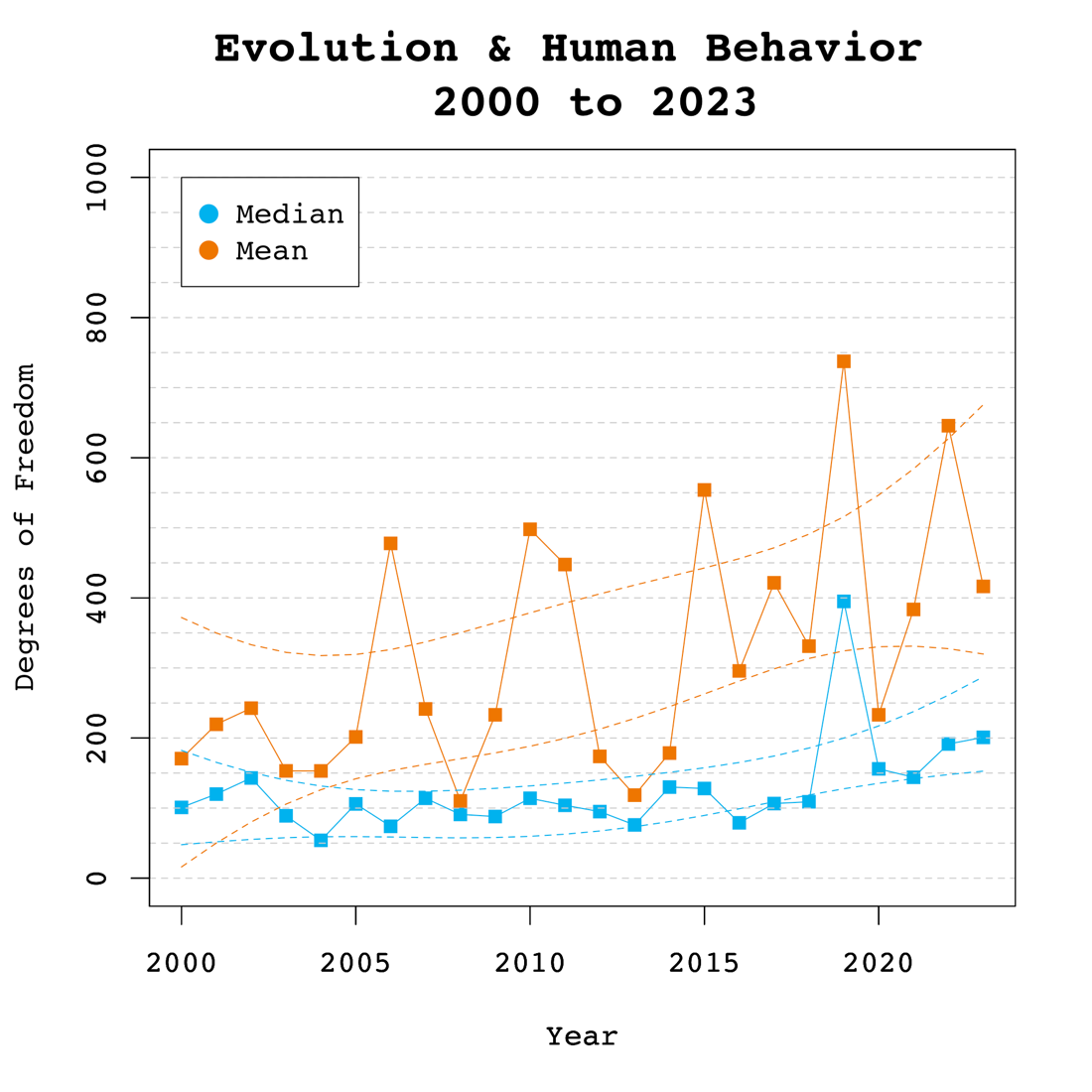
Figure 2 shows the median and mean degrees of freedom used in F-tests and t-tests reported in Evolution & Human Behavior. The mean results are highly variable due to a few studies with extremely large sampel sizes. Thus, we focus on the median to examine time trends. The median degrees of freedom over time was 107.75, ranging from 54 to 395. Regression analyses of the median showed a significant linear increase by 4 to 5 degrees of freedom per year, b = 4.57, SE = 1.69, p = 0.013. However, there was no evidence that the replication crisis influenced a significant increase in sample sizes as seen by the lack of a significant non-linear trend and a small regression coefficient, b = 0.50, SE = 0.27, p = 0.082.
Figure 2
Observed and Expected Discovery Rates
Figure 3 shows the changes in the ODR and EDR estimates over time. There were no significant linear, b = 0.06 (SE = 0.17 p = 0.748) or non-linear, b = -0.02 (SE = 0.03, p = 0.435) trends observed in the ODR estimate. The regression results for the EDR estimate showed no significant linear, b = 0.75 (SE = 0.51 p = 0.153) or non-linear, b = 0.04 (SE = 0.08 p = 0.630) changes over time. These findings indicate the journal has not increased its publication of non-significant results even though selection bias is heavily present. Furthermore, the lack of changes to the EDR suggests that many studies continue to be statistically underpowered to measure the effect sizes of interest.
Figure 3
Expected Replicability Rates and False Discovery Risks
Figure 4 depicts the false discovery risk (FDR) and the Estimated Replication Rate (ERR). It also shows the Expected Replication Failure rate (EFR = 1 – ERR). A comparison of the EFR with the FDR provides information for the interpretation of replication failures. If the FDR is close to the EFR, many replication failures may be due to false positive results in original studies. In contrast, if the FDR is low, most replication failures will likely be false negative results in underpowered replication studies.
The ERR estimate showed a significant linear increase over time, b = 0.61, SE = 0.26, p = 0.031. No significant non-linear trend was observed, b = 0.07, SE = 0.4, p = 0.127. These findings are consistent with the observed significant increase in sample sizes as the reduction in sampling error increases the likelihood that an effect will replicate.
The significant increase in the ERR without a significant increase in the EDR is partially explained by the higher power of the test for the ERR that can be estimated with higher precision. However, it is also possible that the ERR increases more because there is an increase in the heterogeneity of studies. That is, the number of studies with low power has remained constant, but the number of studies with high power has increased. This would result in a bigger increase in the ERR than the EDR.
Figure 4
Visual inspection of Figure 4 depicts the EFR higher than the FDR over time, suggesting that replication failures of studies in Evolution & Human Behavior are more likely to be false negatives rather than false positives. Up to 30% of the published results might not be replicable, and up to 50% of those results may be false positives.
It is noteworthy that the gap between the EFR and the FDR appears to be narrowing over time. This trend is supported by the significant increase in the Estimated Replicability Rate (ERR), where EFR is defined as 1 – ERR. Meanwhile, the Expected Discovery Rate (EDR) has remained constant, indicating that the FDR has also remained unchanged, given that the FDR is derived from a transformation of the EDR. The findings suggest that while original results have become more likely to replicate, the probability that replication failures are false positives remains unchanged.
Adjusting Alpha
A simple solution to a crisis of confidence in published results is to adjust the criterion to reject the null-hypothesis. For example, some researchers have proposed to set alpha to .005 to avoid too many false positive results. With z-curve we can calibrate alpha to keep the false discovery risk at an acceptable level without discarding too many true positive results. To do so, we set alpha to .05, .01, .005, and .001 and examined the false discovery risk.
Figure 5
Figure 5 shows that the conventional criterion of p < .05 produces false discovery risks above 5%. The high variability in annual estimates also makes it difficult to provide precise estimates of the FDR. However, adjusting alpha to .01 is sufficient to produce an FDR with tight confidence intervals below 5%. The benefits of reducing alpha further to .005 or .001 are minimal.
Figure 6
Figure 6 shows the impact of lowering the significance criterion, alpha, on the discovery rate (lower alpha implies fewer significant results). In Evolution & Human Behavior lowering alpha to .01 reduces the observed discovery rate by about 20 percentage points. This implies that 20% of results reported p-values between .05 and .01. These results often have low success rates in actual replication studies (OSC, 2015). Thus, our recommendation is to set alpha to .01 to reduce the false positive risk to 5% and to disregard studies with weak evidence against the null-hypothesis. These studies require actual successful replications with larger samples to provide credible evidence for an evolutionary hypothesis.
There are relatively few studies with p-values between .01 and .005. Thus, more conservative researchers can use alpha = .005 without losing too many additional results.
Limitations
The main limitation of these results is the use of automatically extracted test statistics. This approach cannot distinguish between theoretically important statistical results and other results that are often reported but do not test focal hypotheses (e.g., testing the statistical significance of a manipulation check, reporting a non-significant result for a factor in a complex statistical design that was not expected to produce a significant result).
To examine the influence of automatic extraction on our results, we can compare the results to hand-coding results of over 4,000 hand-coded focal hypotheses in over 40 journals in 2010 and 2020. The ODR was 90% around 2010 and 88% around 2020. Thus, the tendency to report significant results for focal hypothesis tests is even higher than the ODR for all results and there is no indication that this bias has decreased notably over time. The ERR increased a bit from 61% to 67%, but these values are a bit lower than those reported here. Thus, it is possible that focal tests also have lower average power than other tests, but this difference seems to be small. The main finding is that publishing of non-significant results for focal tests remains an exception in psychology journals and probably also in this journal.
One concern about the publication of our results is that it merely creates a new criterion to game publications. Rather than trying to get p-values below .05, researchers may use tricks to get p-values below .01. However, this argument ignores that it becomes increasingly harder to produce lower p-values with tricks (Simmons et al., 2011). Moreover, z-curve analysis makes it easy to see selection bias for different levels of significance. Thus, a more plausible response to these results is that researchers will increase sample sizes or use other methods to reduce sampling error to increase power.
Conclusion
The replicability report for Evolution & Human Behavior suggests that the power to obtain a significant result to report a significant result (i.e., a discovery) ranges from 28% to 71%. This finding suggests that many studies are underpowered and require luck to get a significant result. The false positive risk is modest and can be controlled by setting alpha to .01. Replication attempts of original findings with p-values above .01 should increase sample sizes to produce more conclusive evidence. The journal shows clear evidence of selection bias.
There are several ways, the current or future editors of this journal can improve credibility of results published in this journal. First, results with weak evidence (p-values between .05 and .01) should only be reported as suggestive results that require replication or even request a replication before publication. Second, editors should try to reduce publication bias by prioritizing research questions over results. A well-conducted study with an important question should be published even if the results are not statistically significant. Pre-registration and registered reports can help to reduce publication bias. Editors may also ask for follow-up studies with higher power to follow up on a non-significant result.
Publication bias also implies that point estimates of effect sizes are inflated. It is therefore important to take uncertainty in this estimates into account. Small samples with large sampling error are usually unable to provide meaningful information about effect sizes and conclusions should be limited to the direct of an effect.
The present results serve as a benchmark for future years to track progress in this journal to ensure trust in research by evolutionary psychologists.
“What I’d like to say is that it is OK to criticize a paper, even [if, typo in original] it isn’t horrible.” (Gelman, 2023)
In this spirit, I would like to criticize Loken and Gelman’s confusing article about the interpretation of effect sizes in studies with small samples and selection for significance. They compare random measurement error to a backpack and the outcome of a study to running speed. Common sense suggests that the same individual under identical conditions would run faster without a backpack than with a backpack. The same outcome is also suggested by psychometric theories that suggest random measurement error attenuates population effect sizes, which would make it harder to demonstrate significance and produce, on average, weaker effect sizes.
The key point of Loken and Gelman’s article is to suggest that this intuition fails under some conditions. “Should we assume that if statistical significance is achieved in the presence of measurement error, the associated effects would have been stronger without noise? We caution against the fallacy”
To support their clam that common sense is a fallacy under certain conditions, they present the results of a simple simulation study. After some concerns about their conclusions were raised, Loken and Gelman shared the actual code of their simulation study. In this blog post, I share the code with annotations and reproduce their results. I also show that their results are based on selecting for significance only for the measure with random measurement error (with a backpack) and not for the measure without a backpack (no random measurement error). Reversing the selection shows that selection for significance without measurement error produces stronger effect sizes even more often than selection for significance with a backpack. Thus, it is not a fallacy to assume that we would all run faster without a backpack holding all other factors equal. However, a runner with a heavy backpack and tailwinds might run faster than a runner without a backpack facing strong headwinds. While this is true, the influence of wind on performance makes it difficult to see the influence of the backpack. Under identical conditions backpacks slow people down and random measurement error attenuates effects.
Loken and Gelman’s presentation of the results may explain why some readers, including us, misinterpreted their results to imply that selection bias and random measurement error may interaction in some complex way to produce even more inflated estimates of the true correlation. We added some lines of code to their simulation to compute the average correlations after selection for significance separately for the measure without error and the measure with error. This way, both measures benefit equally from selection bias. The plot also provides more direct evidence about the amount of bias that is introduced by selection bias and random measurement error. In addition, the plot shows the average 95% confidence intervals around the estimated correlation coefficients.
The plot shows that for large samples (N > 1,000), the measure without error always produces the expected true correlation of r = .15, whereas the measure with error always produces the expected attenuated correlation of r = .15 * .80 = .12. As sample sizes get smaller, the effect of selection bias becomes apparent. For the measure without error, the observed effect sizes are now inflated. For the measure with error, selection bias corrects for the inflation and the two biases cancel each other out to produce more accurate estimates of the true effect size than with the measure without error. For sample sizes below N = 400, however, both measures produce inflated estimates and in really small samples the attenuation effect due to unreliability is overwhelmed by selection bias. However, while the difference due to unreliability is negligible and approaches zero, it is clear that random measurement error combined with selection bias never produces even stronger estimates than the measure without error. Thus, it remains true that we should expect a measure without random measurement error to produce stronger correlations than a measure with random error. This fundamental principle of psychometrics, however, does not warrant the conclusion that an observed statistically significant correlation in small samples underestimates the true correlation coefficient because the correlation may have been inflated by selection for significance.
The plot also shows how researchers can avoid misinterpretation of inflated effect size estimates in small samples. In small samples, confidence intervals are wide. Figure 2 shows that the confidence interval around inflated effect size estimates in small samples is so wide that it includes the true correlation of r = .15. The width of the confidence interval in small samples make it clear that the study provided no meaningful information about the size of an effect. This does not mean the results are useless. After all, the results correctly show that the relationship between the variables is positive rather than negative. For the purpose of effect size estimation it is necessary to conduct meta-analysis and to include studies with significant and non-significant results. Furthermore, meta-analysis need to test for the presence of selection bias and correct for it when it is present.
P.S. If somebody claims that they ran a marathon in 2 hours with a heavy backpack, they may not be lying. They may just not tell you all of the information. We often fill in the blanks and that is where things can go wrong. If the backpack were a jet pack and the person was using it to fly for some of the race, we would no longer be surprised by the amazing feat. Similarly, if somebody tells you that they got a correlation of r = .8 in a sample of N = 8 with a measure that has only 20% reliable variance, you should not be surprised if they tell you that they got this result after picking 1 out of 20 studies because selection for significance will produce strong correlations in small samples even if there is no correlation at all. Once they tell you that they tried many times to get the one significant result, it is obvious that the next study is unlikely to replicate a significant result.
Sometimes You Can Be Faster With a Heavy Backpack
Annotated Original Code
### This is the final code used for the simulation studies posted by Andrew Gelman on his blog
### Comments are highlighted with my initials #US#
# First just the original two plots, high power N = 3000, low power N = 50, true slope = .15
r <- .15
sims<-array(0,c(1000,4))
xerror <- 0.5
yerror<-0.5
for (i in 1:1000) {
x <- rnorm(50,0,1)
y <- r*x + rnorm(50,0,1)
#US# this is a sloppy way to simulate a correlation of r = .15
#US# The proper code is r*x + rnorm(50,0,1)*sqrt(1-r^2)
#US# However, with the specific value of r = .15, the difference is trivial
#US# However, however, it raises some concerns about expertise
xx<-lm(y~x)
sims[i,1]<-summary(xx)$coefficients[2,1]
x<-x + rnorm(50,0,xerror)
y<-y + rnorm(50,0,yerror)
xx<-lm(y~x)
sims[i,2]<-summary(xx)$coefficients[2,1]
x <- rnorm(3000,0,1)
y <- r*x + rnorm(3000,0,1)
xx<-lm(y~x)
sims[i,3]<-summary(xx)$coefficients[2,1]
x<-x + rnorm(3000,0,xerror)
y<-y + rnorm(3000,0,yerror)
xx<-lm(y~x)
sims[i,4]<-summary(xx)$coefficients[2,1]
}
plot(sims[,2] ~ sims[,1],ylab=”Observed with added error”,xlab=”Ideal Study”)
abline(0,1,col=”red”)
plot(sims[,4] ~ sims[,3],ylab=”Observed with added error”,xlab=”Ideal Study”)
abline(0,1,col=”red”)
#US# There is no major issue with graphs 1 and 2.
#US# They merely show that high sampling error produces large uncertainty in the estimates.
#US# The small attenuation effect of r = .15 vs. r = 12 is overwhelmed by sampling error
#US# The real issue is the simulation of selection for significance in the third graph
# third graph
# run 2000 regressions at points between N = 50 and N = 3050
r <- .15
propor <-numeric(31)
powers<-seq(50,3050,100)
#US# These lines of code are added to illustrate the biased selection for significane
propor.reversed.selection <-numeric(31)
mean.sig.cor.without.error <- numeric(31) # mean correlation for the measure without error when t > 2
mean.sig.cor.with.error <- numeric(31) # mean correlation for the measure with error when t > 2
#US# It is sloppy to refer to sample sizes as powers.
#US# In between subject studies, the power to produce a true positive result
#US# is a function of the population correlation and the sample size
#US# With population correlations fixed at r = .15 or r = .12, sample size is the
#US# only variable that influences power
#US# However, power varies from alpha to 1 and it would be interesting to compare the
#US# power of studies with r = .15 and r = .12 to produce a significant result.
#US# The claim that “one would always run faster without a backback”
#US# could be interpreted as a claim that it is always easier to obtain a
#US# significant result without measurement error, r = .15, than with measurement error, r = .12
#US# This claim can be tested with Loken and Gelman’s simulation by computing
#US# the percentage of significant results obtained without and with measurement error
#US# Loken and Golman do not show this comparison of power.
#US# The reason might be the confusion of sample size with power.
#US# While sample sizes are held constant, power varies as a function of the population correlations
#US# without, r = .15, and with, r = .12, measurement error.
xerror<-0.5
yerror<-0.5
j = 1
i = 1
for (j in 1:31) {
sims<-array(0,c(1000,4))
for (i in 1:1000) {
x <- rnorm(powers[j],0,1)
y <- r*x + rnorm(powers[j],0,1)
#US# the same sloppy simulation of population correlations as before
xx<-lm(y~x)
sims[i,1:2]<-summary(xx)$coefficients[2,1:2]
x<-x + rnorm(powers[j],0,xerror)
y<-y + rnorm(powers[j],0,yerror)
xx<-lm(y~x)
sims[i,3:4]<-summary(xx)$coefficients[2,1:2]
}
#US# The code is the same as before, it just adds variation in sample sizes
#US# The crucial aspect to understand figure 3 is the following code that
#US# compares the results for the paired outcomes without and with measurement error
#US# Carlos Ungil (https://ch.linkedin.com/in/ungil) pointed out on Gelman’s blog #US# that there is another sloppy mistake in the simulation code that does not alter the results #US# The code compares absolute t-values (coefficient/sampling error), while the article #US# talks about inflated effect size estimates. However, while the sampling error variation #US# creates some variability, the pattern remains the same. #US# For sake of reproducibility I kept the comparison of t-values.
# find significant observations (t test > 2) and then check proportion
temp<-sims[abs(sims[,3]/sims[,4])> 2,]
#US# the use of t > 2 is sloppy and unnecessary.
#US# summary(lm) gives the exact p-values that could be used to select for significance
#US# summary(xx)[2,4] < .05
#US# However, this does not make a substantial difference
#US# The crucial part of this code is that it uses the outcomes of the simulation
#US# with random measurement error to select for significance
#US# As outcomes are paired, this means that the code sometimes selects outcomes
#US# in which sampling error produces significance with random measurement error
The z-curve analysis of results in this journal shows (a) that many published results are based on studies with low to modest power, (b) selection for significance inflates effect size estimates and the discovery rate of reported results, and (c) there is no evidence that research practices have changed over the past decade. Readers should be careful when they interpret results and recognize that reported effect sizes are likely to overestimate real effect sizes, and that replication studies with the same sample size may fail to produce a significant result again. To avoid misleading inferences, I suggest using alpha = .005 as a criterion for valid rejections of the null-hypothesis. Using this criterion, the risk of a false positive result is below 2%. I also recommend computing a 99% confidence interval rather than the traditional 95% confidence interval for the interpretation of effect size estimates.
Given the low power of many studies, readers also need to avoid the fallacy to report non-significant results as evidence for the absence of an effect. With 50% power, the results can easily switch in a replication study so that a significant result becomes non-significant and a non-significant result becomes significant. However, selection for significance will make it more likely that significant results become non-significant than observing a change in the opposite direction.
The average power of studies in a heterogeneous journal like Frontiers of Psychology provides only circumstantial evidence for the evaluation of results. When other information is available (e.g., z-curve analysis of a discipline, author, or topic, it may be more appropriate to use this information).
Report
Frontiers of Psychology was created in 2010 as a new online-only journal for psychology. It covers many different areas of psychology, although some areas have specialized Frontiers journals like Frontiers in Behavioral Neuroscience.
The business model of Frontiers journals relies on publishing fees of authors, while published articles are freely available to readers.
The number of articles in Frontiers of Psychology has increased quickly from 131 articles in 2010 to 8,072 articles in 2022 (source Web of Science). With over 8,000 published articles Frontiers of Psychology is an important outlet for psychological researchers to publish their work. Many specialized, print-journals publish fewer than 100 articles a year. Thus, Frontiers of Psychology offers a broad and large sample of psychological research that is equivalent to a composite of 80 or more specialized journals.
Another advantage of Frontiers of Psychology is that it has a relatively low rejection rate compared to specialized journals that have limited journal space. While high rejection rates may allow journals to prioritize exceptionally good research, articles published in Frontiers of Psychology are more likely to reflect the common research practices of psychologists.
To examine the replicability of research published in Frontiers of Psychology, I downloaded all published articles as PDF files, converted PDF files to text files, and extracted test-statistics (F, t, and z-tests) from published articles. Although this method does not capture all published results, there is no a priori reason that results reported in this format differ from other results. More importantly, changes in research practices such as higher power due to larger samples would be reflected in all statistical tests.
As Frontiers of Psychology only started shortly before the replication crisis in psychology increased awareness about the problem of low statistical power and selection for significance (publication bias), I was not able to examine replicability before 2011. I also found little evidence of changes in the years from 2010 to 2015. Therefore, I use this time period as the starting point and benchmark for future years.
Figure 1 shows a z-curve plot of results published from 2010 to 2014. All test-statistics are converted into z-scores. Z-scores greater than 1.96 (the solid red line) are statistically significant at alpha = .05 (two-sided) and typically used to claim a discovery (rejection of the null-hypothesis). Sometimes even z-scores between 1.65 (the dotted red line) and 1.96 are used to reject the null-hypothesis either as a one-sided test or as marginal significance. Using alpha = .05, the plot shows 71% significant results, which is called the observed discovery rate (ODR).
Visual inspection of the plot shows a peak of the distribution right at the significance criterion. It also shows that z-scores drop sharply on the left side of the peak when the results do not reach the criterion for significance. This wonky distribution cannot be explained with sampling error. Rather it shows a selective bias to publish significant results by means of questionable practices such as not reporting failed replication studies or inflating effect sizes by means of statistical tricks. To quantify the amount of selection bias, z-curve fits a model to the distribution of significant results and estimates the distribution of non-significant (i.e., the grey curve in the range of non-significant results). The discrepancy between the observed distribution and the expected distribution shows the file-drawer of missing non-significant results. Z-curve estimates that the reported significant results are only 31% of the estimated distribution. This is called the expected discovery rate (EDR). Thus, there are more than twice as many significant results as the statistical power of studies justifies (71% vs. 31%). Confidence intervals around these estimates show that the discrepancy is not just due to chance, but active selection for significance.
Using a formula developed by Soric (1989), it is possible to estimate the false discovery risk (FDR). That is, the probability that a significant result was obtained without a real effect (a type-I error). The estimated FDR is 12%. This may not be alarming, but the risk varies as a function of the strength of evidence (the magnitude of the z-score). Z-scores that correspond to p-values close to p =.05 have a higher false positive risk and large z-scores have a smaller false positive risk. Moreover, even true results are unlikely to replicate when significance was obtained with inflated effect sizes. The most optimistic estimate of replicability is the expected replication rate (ERR) of 69%. This estimate, however, assumes that a study can be replicated exactly, including the same sample size. Actual replication rates are often lower than the ERR and tend to fall between the EDR and ERR. Thus, the predicted replication rate is around 50%. This is slightly higher than the replication rate in the Open Science Collaboration replication of 100 studies which was 37%.
Figure 2 examines how things have changed in the next five years.
The observed discovery rate decreased slightly, but statistically significantly, from 71% to 66%. This shows that researchers reported more non-significant results. The expected discovery rate increased from 31% to 40%, but the overlapping confidence intervals imply that this is not a statistically significant increase at the alpha = .01 level. (if two 95%CI do not overlap, the difference is significant at around alpha = .01). Although smaller, the difference between the ODR of 60% and the EDR of 40% is statistically significant and shows that selection for significance continues. The ERR estimate did not change, indicating that significant results are not obtained with more power. Overall, these results show only modest improvements, suggesting that most researchers who publish in Frontiers in Psychology continue to conduct research in the same way as they did before, despite ample discussions about the need for methodological reforms such as a priori power analysis and reporting of non-significant results.
The results for 2020 show that the increase in the EDR was a statistical fluke rather than a trend. The EDR returned to the level of 2010-2015 (29% vs. 31), but the ODR remained lower than in the beginning, showing slightly more reporting of non-significant results. The size of the file drawer remains large with an ODR of 66% and an EDR of 72%.
The EDR results for 2021 look again better, but the difference to 2020 is not statistically significant. Moreover, the results in 2022 show a lower EDR that matches the EDR in the beginning.
Overall, these results show that results published in Frontiers in Psychology are selected for significance. While the observed discovery rate is in the upper 60%s, the expected discovery rate is around 35%. Thus, the ODR is nearly twice the rate of the power of studies to produce these results. Most concerning is that a decade of meta-psychological discussions about research practices has not produced any notable changes in the amount of selection bias or the power of studies to produce replicable results.
How should readers of Frontiers in Psychology articles deal with this evidence that some published results were obtained with low power and inflated effect sizes that will not replicate? One solution is to retrospectively change the significance criterion. Comparisons of the evidence in original studies and replication outcomes suggest that studies with a p-value below .005 tend to replicate at a rate of 80%, whereas studies with just significant p-values (.050 to .005) replicate at a much lower rate (Schimmack, 2022). Demanding stronger evidence also reduces the false positive risk. This is illustrated in the last figure that uses results from all years, given the lack of any time trend.
In the Figure the red solid line moved to z = 2.8; the value that corresponds to p = .005, two-sided. Using this more stringent criterion for significance, only 45% of the z-scores are significant. Another 25% were significant with alpha = .05, but are no longer significant with alpha = .005. As power decreases when alpha is set to more stringent, lower, levels, the EDR is also reduced to only 21%. Thus, there is still selection for significance. However, the more effective significance filter also selects for more studies with high power and the ERR remains at 72%, even with alpha = .005 for the replication study. If the replication study used the traditional alpha level of .05, the ERR would be even higher, which explains the finding that the actual replication rate for studies with p < .005 is about 80%.
The lower alpha also reduces the risk of false positive results, even though the EDR is reduced. The FDR is only 2%. Thus, the null-hypothesis is unlikely to be true. The caveat is that the standard null-hypothesis in psychology is the nil-hypothesis and that the population effect size might be too small to be of practical significance. Thus, readers who interpret results with p-values below .005 should also evaluate the confidence interval around the reported effect size, using the more conservative 99% confidence interval that correspondence to alpha = .005 rather than the traditional 95% confidence interval. In many cases, this confidence interval is likely to be wide and provide insufficient information about the strength of an effect.
Since 2011, it is an open secret that many published results in psychology journals do not replicate. The replicability of published results is particularly low in social psychology (Open Science Collaboration, 2015).
A key reason for low replicability is that researchers are rewarded for publishing as many articles as possible without concerns about the replicability of the published findings. This incentive structure is maintained by journal editors, review panels of granting agencies, and hiring and promotion committees at universities.
To change the incentive structure, I developed the Replicability Index, a blog that critically examined the replicability, credibility, and integrity of psychological science. In 2016, I created the first replicability rankings of psychology departments (Schimmack, 2016). Based on scientific criticisms of these methods, I have improved the selection process of articles to be used in departmental reviews.
1. I am using Web of Science to obtain lists of published articles from individual authors (Schimmack, 2022). This method minimizes the chance that articles that do not belong to an author are included in a replicability analysis. It also allows me to classify researchers into areas based on the frequency of publications in specialized journals. Currently, I cannot evaluate neuroscience research. So, the rankings are limited to cognitive, social, developmental, clinical, and applied psychologists.
2. I am using department’s websites to identify researchers that belong to the psychology department. This eliminates articles that are from other departments.
3. I am only using tenured, active professors. This eliminates emeritus professors from the evaluation of departments. I am not including assistant professors because the published results might negatively impact their chances to get tenure. Another reason is that they often do not have enough publications at their current university to produce meaningful results.
Like all empirical research, the present results rely on a number of assumptions and have some limitations. The main limitations are that (a) only results that were found in an automatic search are included (b) only results published in 120 journals are included (see list of journals) (c) published significant results (p < .05) may not be a representative sample of all significant results (d) point estimates are imprecise and can vary based on sampling error alone.
These limitations do not invalidate the results. Large difference in replicability estimates are likely to predict real differences in success rates of actual replication studies (Schimmack, 2022).
New York University
I used the department website to find core members of the psychology department. I found 13 professors and 6 associate professors. Figure 1 shows the z-curve for all 12,365 tests statistics in articles published by these 19 faculty members. I use the Figure to explain how a z-curve analysis provides information about replicability and other useful meta-statistics.
1. All test-statistics are converted into absolute z-scores as a common metric of the strength of evidence (effect size over sampling error) against the null-hypothesis (typically H0 = no effect). A z-curve plot is a histogram of absolute z-scores in the range from 0 to 6. The 1,239 (~ 10%) of z-scores greater than 6 are not shown because z-scores of this magnitude are extremely unlikely to occur when the null-hypothesis is true (particle physics uses z > 5 for significance). Although they are not shown, they are included in the meta-statistics.
2. Visual inspection of the histogram shows a steep drop in frequencies at z = 1.96 (dashed blue/red line) that corresponds to the standard criterion for statistical significance, p = .05 (two-tailed). This shows that published results are selected for significance. The dashed red/white line shows significance for p < .10, which is often used for marginal significance. There is another drop around this level of significance.
3. To quantify the amount of selection bias, z-curve fits a statistical model to the distribution of statistically significant results (z > 1.96). The grey curve shows the predicted values for the observed significant results and the unobserved non-significant results. The full grey curve is not shown to present a clear picture of the observed distribution. The statistically significant results (including z > 6) make up 20% of the total area under the grey curve. This is called the expected discovery rate because the results provide an estimate of the percentage of significant results that researchers actually obtain in their statistical analyses. In comparison, the percentage of significant results (including z > 6) includes 70% of the published results. This percentage is called the observed discovery rate, which is the rate of significant results in published journal articles. The difference between a 70% ODR and a 20% EDR provides an estimate of the extent of selection for significance. The difference of 50 percentage points is large. The upper level of the 95% confidence interval for the EDR is 28%. Thus, the discrepancy is not just random. To put this result in context, it is possible to compare it to the average for 120 psychology journals in 2010 (Schimmack, 2022). The ODR is similar (70 vs. 72%), but the EDR is a bit lower (20% vs. 28%), although the difference might be largely due to chance.
4. The EDR can be used to estimate the risk that published results are false positives (i.e., a statistically significant result when H0 is true), using Soric’s (1989) formula for the maximum false discovery rate. An EDR of 20% implies that no more than 20% of the significant results are false positives, however the upper limit of the 95%CI of the EDR, 28%, allows for 36% false positive results. Most readers are likely to agree that this is an unacceptably high risk that published results are false positives. One solution to this problem is to lower the conventional criterion for statistical significance (Benjamin et al., 2017). Figure 2 shows that alpha = .005 reduces the point estimate of the FDR to 3% with an upper limit of the 95% confidence interval of XX%. Thus, without any further information readers could use this criterion to interpret results published by NYU faculty members.
5. The estimated replication rate is based on the mean power of significant studies (Brunner & Schimmack, 2020). Under ideal condition, mean power is a predictor of the success rate in exact replication studies with the same sample sizes as the original studies. However, as NYU professor van Bavel pointed out in an article, replication studies are never exact, especially in social psychology (van Bavel et al., 2016). This implies that actual replication studies have a lower probability of producing a significant result, especially if selection for significance is large. In the worst case scenario, replication studies are not more powerful than original studies before selection for significance. Thus, the EDR provides an estimate of the worst possible success rate in actual replication studies. In the absence of further information, I have proposed to use the average of the EDR and ERR as a predictor of actual replication outcomes. With an ERR of 62% and an EDR of 20%, this implies an actual replication prediction of 41%. This is close to the actual replication rate in the Open Science Reproducibility Project (Open Science Collaboration, 2015). The prediction for results published in 120 journals in 2010 was (ERR = 67% + ERR = 28%)/ 2 = 48%. This suggests that results published by NYU faculty are slightly less replicable than the average result published in psychology journals, but the difference is relatively small and might be mostly due to chance.
6. There are two reasons for low replication rates in psychology. One possibility is that psychologists test many false hypotheses (i.e., H0 is true) and many false positive results are published. False positive results have a very low chance of replicating in actual replication studies (i.e. 5% when .05 is used to reject H0), and will lower the rate of actual replications a lot. Alternative, it is possible that psychologists tests true hypotheses (H0 is false), but with low statistical power (Cohen, 1961). It is difficult to distinguish between these two explanations because the actual rate of false positive results is unknown. However, it is possible to estimate the typical power of true hypotheses tests using Soric’s FDR. If 20% of the significant results are false positives, the power of the 80% true positives has to be (.62 – .2*.05)/.8 = 76%. This would be close to Cohen’s recommended level of 80%, but with a high level of false positive results. Alternatively, the null-hypothesis may never be really true. In this case, the ERR is an estimate of the average power to get a significant result for a true hypothesis. Thus, power is estimated to be between 62% and 76%. The main problem is that this is an average and that many studies have less power. This can be seen in Figure 1 by examining the local power estimates for different levels of z-scores. For z-scores between 2 and 2.5, the ERR is only 47%. Thus, many studies are underpowered and have a low probability of a successful replication with the same sample size even if they showed a true effect.
Area
The results in Figure 1 provide highly aggregated information about replicability of research published by NYU faculty. The following analyses examine potential moderators. First, I examined social and cognitive research. Other areas were too small to be analyzed individually.
The z-curve for the 11 social psychologists was similar to the z-curve in Figure 1 because they provided more test statistics and had a stronger influence on the overall result.
The z-curve for the 6 cognitive psychologists looks different. The EDR and ERR are higher for cognitive psychology, and the 95%CI for social and cognitive psychology do not overlap. This suggests systematic differences between the two fields. These results are consistent with other comparisons of the two fields, including actual replication outcomes (OSC, 2015). With an EDR of 44%, the false discovery risk for cognitive psychology is only 7% with an upper limit of the 95%CI at 12%. This suggests that the conventional criterion of .05 does keep the false positive risk at a reasonably low level or that an adjustment to alpha = .01 is sufficient. In sum, the results show that results published by cognitive researchers at NYU are more replicable than those published by social psychologists.
Position
Since 2015 research practices in some areas of psychology, especially social psychology, have changed to increase replicability. This would imply that research by younger researchers is more replicable than research by more senior researchers that have more publications before 2015. A generation effect would also imply that a department’s replicability increases when older faculty members retire. On the other hand, associate professors are relatively young and likely to influence the reputation of a department for a long time.
The figure above shows that most test statistics come from the (k = 13) professors. As a result, the z-curve looks similar to the z-curve for all test values in Figure 1. The results for the 6 associate professors (below) are more interesting. Although five of the six associate professors are in the social area, the z-curve results show a higher EDR and less selection bias than the plot for all social psychologists. This suggests that the department will improve when full professors in social psychology retire.
Some researchers have changed research practices in response to the replication crisis. It is therefore interesting to examine whether replicability of newer research has improved. To examine this question, I performed a z-curve analysis for articles published in the past five year (2016-2021).
The results show very little signs of improvement. The EDR increased from 20% to 26%, but the confidence intervals are too wide to infer that this is a systematic change. In contrast, Stanford University improved from 22% to 50%, a significant increase. For now, NYU results should be interpreted with alpha = .005 as threshold for significance to maintain a reasonable false positive risk.
The table below shows the meta-statistics of all 19 faculty members. You can see the z-curve for each faculty member by clicking on their name.
Gordon et al. (2021) conducted a meta-analysis of 103 studies that were included in prediction markets to forecast the outcome of replication studies. The results show that prediction markets can forecast replication outcomes above chance levels, but the value of this information is limited. Without actual replication studies, it remains unclear which published results can be trusted or not. Here I compare the performance of prediction markets to the R-Index and the closely related p < .005 rule. These statistical forecasts perform nearly as well as markets and are much easier to use to make sense of thousands of published articles. However, even these methods have a high failure rate. The best solution to this problem is to rely on meta-analyses of studies rather than to predict the outcome of a single study. In addition to meta-analyses, it will be necessary to conduct new studies that are conducted with high scientific integrity to provide solid empirical foundations for psychology. Claims that are not supported by bias-corrected meta-analyses or new preregistered studies are merely suggestive and currently lack empirical support.
Introduction
Since 2011, it became apparent that many published results in psychology, especially social psychology fail to replicate in direct replication studies (Open Science Collaboration, 2015). In social psychology the success rate of replication studies is so low (25%) that it makes sense to bet on replication failures. This would produce 75% successful outcomes, but it would also imply that an entire literature has to be discarded.
It is practically impossible to redo all of the published studies to assess their replicability. Thus, several projects have attempted to predict replication outcomes of individual studies. One strategy is to conduct prediction markets in which participants can earn real money by betting on replication outcomes. There have been four prediction markets with a total of 103 studies with known replication outcomes (Gordon et al., 2021). The key findings are summarized in Table 1.
Markets have a good overall success rate, (28+47)/103 = 73% that is above chance (flipping a coin). Prediction markets are better at predicting failures, 28/31 = 90%, than predicting successes, 47/72 = 65%. The modest success rate for success is a problem because it would be more valuable to be able to identify studies that will replicate and do not require a new study to verify the results.
Another strategy to predict replication outcomes relies on the fact that the p-values of original studies and the p-values of replication studies are influenced by the statistical power of a study (Brunner & Schimmack, 2020). Studies with higher power are more likely to produce lower p-values and more likely to produce significant p-values in replication studies. As a result, p-values also contain valuable information about replication outcomes. Gordon et al. (2021) used p < .005 as a rule to predict replication outcomes. Table 2 shows the performance of this simple rule.
The overall success rate of this rule is nearly as good as the prediction markets, (39+35)/103 = 72%; a difference by k = 1 studies. The rule does not predict failures as well as the markets, 39/54 = 72% (vs. 90%), but it predicts successes slightly better than the markets, 35/49 = 71% (vs. 65%).
A logistic regression analysis showed that both predictors independently contribute to the prediction of replication outcomes, market b = 2.50, se = .68, p = .0002; p < .005 rule: b = 1.44, se = .48, p = .003.
In short, p-values provide valuable information about the outcome of replication studies.
The R-Index
Although a correlation between p-values and replication outcomes follows logically from the influence of power on p-values in original and replication studies, the cut-off value of .005 appears to be arbitrary. Gordon et al. (2017) justify its choice with an article by Benjamin et al. (2017) that recommended a lower significance level (alpha) to ensure a lower false positive risk. Moreover, they advocated for this rule for new studies that preregister hypotheses and do not suffer from selection bias. In contrast, the replication crisis was caused by selection for significance which produced success rates of 90% or more in psychology journals (Motyl et al., 2017; Sterling, 1959; Sterling et al., 1995). One main reason for replication failures is that selection for significance inflates effect sizes and due to regression to the mean, effect sizes in replication studies are bound to be weaker, resulting in non-significant results, especially if the original p-value was close to the threshold value of alpha = .05. The Open Science Collaboration (2015) replicability project showed that effect sizes are on average inflated by over 100%.
The R-Index provides a theoretical rational for the choice of a cut-off value for p-values. The theoretical cutoff value happens to be p = .0084. The fact that it is close to Benjamin et al.’s (2017) value of .005 is merely a coincidence.
P-values can be transformed into estimates of the statistical power of a study. These estimates rely on the observed effect size of a study and are sometimes called observed power or post-hoc power because power is computed after the results of a study are known. Figure 1 illustrates observed power with an example of a z-test that produced a z-statistic of 2.8 which corresponds to a two-sided p-value of .005.
A p-value of .005 corresponds to z-value of 2.8 for the standard normal distribution centered over zero (the nil-hypothesis). The standard level of statistical significance, alpha = .05 (two-sided) corresponds to z-value of 1.96. Figure 1 shows the sampling distribution of studies with a non-central z-score of 2.8. The green line cuts this distribution into a smaller area of 20% below the significance level and a larger area of 80% above the significance level. Thus, the observed power is 80%.
Selection for significance implies truncating the normal distribution at the level of significance. This means the 20% of non-significant results are discarded. As a result, the median of the truncated distribution is higher than the median of the full normal distribution. The new median can be found using the truncnorm package in R.
qtruncnorm(.5,a = qnorm(1-.05/2),mean=2.8) = 3.05
This value corresponds to an observed power of
qnorm(3.05,qnorm(1-.05/2) = .86
Thus, selection for significance inflates observed power of 80% to 86%. The amount of inflation is larger when power is lower. With 20% power, the inflated power after selection for significance is 67%.
Figure 3 shows the relationship between inflated power on the x-axis and adjusted power on the y-axis. The blue curve uses the truncnorm package. The green line shows the simplified R-Index that simply substracts the amount of inflation from the inflated power. For example, if inflated power is 86%, the inflation is 1-.86 = 14% and subtracting the inflation gives an R-Index of 86-14 = 82%. This is close to the actual value of 80% that produced the inflated value of 86%.
Figure 4 shows that the R-Index is conservative (underestimates power) when power is over 50%, but is liberal (overestimates power) when power is below 50%. The two methods are identical when power is 50% and inflated power is 75%. This is a fortunate co-incidence because studies with more than 50% power are expected to replicate and studies with less than 50% power are expected to fail in a replication attempt. Thus, the simple R-Index makes the same dichotomous predictions about replication outcomes as the more sophisticated approach to find the median of the truncated normal distribution.
The inflated power for actual power of 50% is 75% and 75% power corresponds to a z-score of 2.63, which in turn corresponds to a p-value of p = .0084.
Performance of the R-Index is slightly worse than the p < .005 rule because the R-Index predicts 5 more successes, but 4 of these predictions are failures. Given the small sample size, it is not clear whether this difference is reliable.
In sum, the R-Index is based on a transformation of p-values into estimates of statistical power, while taking into account that observed power is inflated when studies are selected for significance. It provides a theoretical rational for the atheoretical p < .005 rule, because this rule roughly cuts p-values into p-values with more or less than 50% power.
Predicting Success Rates
The overall success rate across the 103 replication studies was 50/103 = 49%. This percentage cannot be generalized to a specific population of studies because the 103 are not a representative sample of studies. Only the Open Science Collaboration project used somewhat representative sampling. However, the 49% success rate can be compared to the success rates of different prediction methods. For example, prediction markets predict a success rate of 72/103 = 70%, a significant difference (Gordon et al., 2021). In contrast, the R-Index predicts a success rate of 54/103 = 52%, which is closer to the actual success rate. The p < .005 rule does even better with a predicted success rate of 49/103 = 48%.
Another method that has been developed to estimate the expected replication rate is z-curve (Bartos & Schimmack, 2021; Brunner & Schimmack, 2020). Z-curve transforms p-values into z-scores and then fits a finite mixture model to the distribution of significant p-values. Figure 5 illustrates z-curve with the p-values from the 103 replicated studies.
The z-curve estimate of the expected replication rate is 60%. This is better than the prediction market, but worse than the R-Index or the p < .005 rule. However, the 95%CI around the ERR includes the true value of 49%. Thus, sampling error alone might explain this discrepancy. However, Bartos and Schimmack (2021) discussed several other reasons why the ERR may overestimate the success rate of actual replication studies. One reason is that actual replication studies are not perfect replicas of the original studies. So called, hidden moderators may create differences between original and replication studies. In this case, selection for significance produces even more inflation that the model assumes. In the worst case scenario, a better estimate of actual replication outcomes might be the expected discovery rate (EDR), which is the power of all studies that were conducted, including non-significant studies. The EDR for the 103 studies is 28%, but the 95%CI is wide and includes the actual rate of 49%. Thus, the dataset is too small to decide between the ERR or the EDR as best estimates of actual replication outcomes. At present it is best to consider the EDR the worst possible and the ERR the best possible scenario and to expect the actual replication rate to fall within this interval.
Social Psychology
The 103 studies cover studies from experimental economics, cognitive psychology, and social psychology. Social psychology has the largest set of studies (k = 54) and the lowest success rate, 33%. The prediction markets overpredict successes, 50%. The R-Index also overpredicted successes, 46%. The p < .005 rule had the least amount of bias, 41%.
Z-curve predicted an ERR of 55% s and the actual success rate fell outside the 95% confidence interval, 34% to 74%. The EDR of 22% underestimates the success rate, but the 95%CI is wide and includes the true value, 95%CI = 5% to 70%. Once more the actual success rate is between the EDR and the ERR estimates, 22% < 34% < 55%.
In short, prediction models appear to overpredict replication outcomes in social psychology. One reason for this might be that hidden moderators make it difficult to replicate studies in social psychology which adds additional uncertainty to the outcome of replication studies.
Regarding predictions of individual studies, prediction markets achieved an overall success rate of 76%. Prediction markets were good at predicting failures, 25/27 = 93%, but not so good in predicting successes, 16/27 = 59%.
The R-Index performed as well as the prediction markets with one more prediction of a replication failure.
The p < .005 rule was the best predictor because it predicted more replication failures.
Performance could be increased by combining prediction markets and the R-Index and only bet on successes when both predictors predicted a success. In particular, the prediction of success improved to 14/19 = 74%. However, due to the small sample size it is not clear whether this is a reliable finding.
Non-Social Studies
The remaining k = 56 studies had a higher success rate, 65%. The prediction markets overpredicted success, 92%. The R-Index underpredicted successes, 59%. The p < .005 rule underpredicted successes even more.
This time z-curve made the best prediction with an ERR of 67%, 95%CI = 45% to 86%. The EDR underestimates the replication rate, although the 95%CI is very wide and includes the actual success rate, 5% to 81%. The fact that z-curve overestimated replicability for social psychology, but not for other areas, suggests that hidden moderators may contribute to the replication problems in social psychology.
For predictions of individual outcomes, prediction markets had a success rate of (3 + 31)/49 = 76%. The good performance is due to the high success rate. Simply betting on success would have produced 32/49 = 65% successes. Predictions of failures had a s success rate of 3/4 = 75% and predictions of successes had a success rate of 31/45 = 69%.
The R-Index had a lower success rate of (9 +21)/49 = 61%. The R-Index was particularly poor at predicting failures, 9/20 = 45%, but was slightly better at predicting successes than the prediction markets, 21/29 = 72%.
The p < .500 rule had a success rate equal to the R-Index, (10 + 20)/49 = 61%, with one more correctly predicted failure and one less correctly predicted success.
Discussion
The present results reproduce the key findings of Gordon et al. (2021). First, prediction markets overestimate the success of actual replication studies. Second, prediction markets have some predictive validity in forecasting the outcome of individual replication studies. Third, a simple rule based on p-values also can forecast replication outcomes.
The present results also extend Gordon et al.’s (2021) findings based on additional analyses. First, I compared the performance of prediction markets to z-curve as a method for the prediction of the success rates of replication outcomes (Bartos & Schimmack, 2021; Brunner & Schimmack, 2021). Z-curve overpredicted success rates for all studies and for social psychology, but was very accurate for the remaining studies (economics, cognition). In all three comparisons, z-curve performed better than prediction markets. Z-curve also has several additional advantages over prediction markets. First, it is much easier to code a large set of test statistics than to run prediction markets. As a result, z-curve has already been used to estimate the replication rates for social psychology based on thousands of test statistics, whereas estimates of prediction markets are based on just over 50 studies. Second, z-curve is based on sound statistical principles that link the outcomes of original studies to the outcomes of replication studies (Brunner & Schimmack, 2020). In contrast, prediction markets rest on unknown knowledge of market participants that can vary across markets. Third, z-curve estimates are provided with validated information about the uncertainty in the estimates, whereas prediction markets provide no information about uncertainty and uncertainty is large because markets tend to be small. In conclusion, z-curve is more efficient and provides better estimates of replication rates than prediction markets.
The main goal of prediction markets is to assess the credibility of individual studies. Ideally, prediction markets would help consumers of published research to distinguish between studies that produced real findings (true positives) and studies that produced false findings (false positives) without the need to run additional studies. The encouraging finding is that prediction markets have some predictive validity and can distinguish between studies that replicate and studies that do not replicate. However, to be practically useful it is necessary to assess the practical usefulness of the information that is provided by prediction markets. Here we need to distinguish the practical consequences of replication failures and successes. Within the statistical framework of nil-hypothesis significance testing, successes and failures have different consequences.
A replication failure increases uncertainty about the original finding. Thus, more research is needed to understand why the results diverged. This is also true for market predictions. Predictions that a study would fail to replicate cast doubt about the original study, but do not provide conclusive evidence that the original study reported a false positive result. Thus, further studies are needed, even if a market predicts a failure. In contrast, successes are more informative. Replicating a previous finding successfully strengthens the original findings and provides fairly strong evidence that a finding was not a false positive result. Unfortunately, the mere prediction that a finding will replicate does not provide the same reassurance because markets only have an accuracy of about 70% when they predict a successful replication. The p < .500 rule is much easier to implement, but its ability to forecast successes is also around 70%. Thus, neither markets nor a simple statistical rule are accurate enough to avoid actual replication studies.
Meta-Analysis
The main problem of prediction markets and other forecasting projects is that single studies are rarely enough to provide evidence that is strong enough to evaluate theoretical claims. It is therefore not particularly important whether one study can be replicated successfully or not, especially when direct replications are difficult or impossible. For this reason, psychologists have relied for a long time on meta-analyses of similar studies to evaluate theoretical claims.
It is surprising that prediction markets have forecasted the outcome of studies that have been replicated many times before the outcome of a new replication study was predicted. Take the replication of Schwarz, Strack, and Mai (1991) in Many Labs 2 as an example. This study manipulated the item-order of questions about marital satisfaction and life-satisfaction and suggested that a question about marital satisfaction can prime information that is used in life-satisfaction judgments. Schimmack and Oishi (2005) conducted a meta-analysis of the literature and showed that the results by Schwarz et al. (1991) were unusual and that the actual effect size is much smaller. Apparently, the market participants were unaware of this meta-analysis and predicted that the original result would replicate successfully (probability of success = 72%). Contrary to the market, the study failed to replicate. This example suggests that meta-analyses might be more valuable than prediction markets or the p-value of a single study.
The main obstacle for the use of meta-analyses is that many published meta-analyses fail to take selection for significance into account and overestimate replicability. However, new statistical methods that correct for selection bias may address this problem. The R-Index is a rather simple tool that allows to correct for selection bias in small sets of studies. I use the article by Nairne et al. (2008) that was used for the OSC project as an example. The replication project focused on Study 2 that produced a p-value of .026. Based on this weak evidence alone, the R-Index would predict a replication failure (observed power = .61, inflation = .39, R-Index = .61 – .39 = .22). However, Study 1 produced much more convincing evidence for the effect, p = .0007. If this study had been picked for the replication attempt, the R-Index would have predicted a successful outcome (observed power = .92, inflation = .08, R-Index = .84). A meta-analysis would average across the two power estimates and also predict a successful replication outcome (mean observed power = .77, inflation = .23, R-Index = .53). The actual replication study was significant with p = .007 (observed power = .77, inflation = .23, R-Index = .53). A meta-analysis across all three studies also suggests that the next study will be a successful replication (R-Index = .53), but the R-Index also shows that replication failures are likely because the studies have relatively low power. In short, prediction markets may be useful when only a single study is available, but meta-analysis are likely to be superior predictors of replication outcomes when prior replication studies are available.
Conclusion
Gordon et al. (2021) conducted a meta-analysis of 103 studies that were included in prediction markets to forecast the outcome of replication studies. The results show that prediction markets can forecast replication outcomes above chance levels, but the value of this information is limited. Without actual replication studies, it remains unclear which published results can be trusted or not. Statistical methods that simply focus on the strength of evidence in original studies perform nearly as well and are much easier to use to make sense of thousands of published articles. However, even these methods have a high failure rate. The best solution to this problem is to rely on meta-analyses of studies rather than to predict the outcome of a single study. In addition to meta-analyses, it will be necessary to conduct new studies that are conducted with high scientific integrity to provide solid empirical foundations for psychology.
Cookie Consent
We use cookies to improve your experience on our site. By using our site, you consent to cookies.