Summary

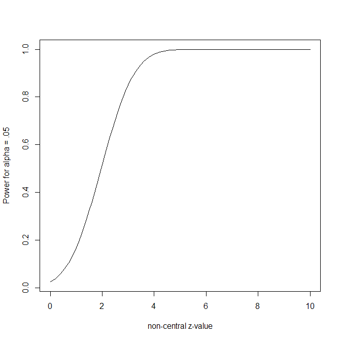
For method folks, the picture tells the full story: z-curve can estimate the true mean of a set of heterogeneous studies better than the weight-function model because the weight function model makes unrealistic assumptions about the distribution of population effect sizes. Added bonus: z-curves estimates are related to actual studies, whereas the estimates of weightr are population estimates that are not connected to the actual studies.
Try it: TMT analysis with z-curve.3.86
The Long Story
The root cause of the crises in psychology is poor training in scientific thinking and scientific methods. Period! I know because I have been teaching at a top-ranked university in North America for over 25 years now. The most common criticism in student evaluations is that my courses are not psychology courses, but statistics course. The reason: I use numbers when I present research findings. But most students can get a degree in psychology without using numbers. Graduate education does not help because students learn from a mentor, who also never learned to think quantitatively. So, psychology is the worst of both worlds. It is neither qualitative research that pays attention to people’s thoughts, feelings, or actual behaviors, nor is it a quantitative science that use valid quantitative information for the same purpose. It is a pseudo-science that produces meaningless numbers that mainly serve the purpose of claiming scientific support for researchers’ personal beliefs.
The problem that quantitative results in published articles cannot be trusted is now widely recognized and has been called a crisis of confidence a credibility crisis, or the replication crisis. However, the problem also exists at the meta-level when questionable published results are combined into a meta-analysis. Don’t get me wrong. Meta-analysis, like all statistical models, are not wrong. They are only wrong when incompetent researchers use these tools without understand how they work and what assumptions these models make.
Meta-analysis is easy to understand and perform when all data are available. We simply combine summary statistics to reduce sampling error and get a more precise estimate of the population effect size. Instead of running one study with N = 1,000 participants, we combine data from 25 studies with 40 participants. The result is practically the same. However, in psychology, the 25 published study are only a fraction of studies that were conducted and produced a significant result (Sterling et al., 1995). This means the effect sizes in the studies are inflated by publication bias and the same bias leads to an inflated effect size estimate in the meta-analysis. Thus, normal meta-analysis that ignore bias are as useful as a wet tissue paper on a 40°C (104°F) day in the middle of a parking lot at noon.
The solution to this problem is to use fancy statistical models that promise to correct for these biases and reveal the truth hidden in a pile of selected and p-hacked studies. The simple truth is that this goal is as attainable as making gold from base metals. However, as readers also do not understand these models and the problem of using them with uninformative data, the results are now routinely included in meta-analytic articles, if only as a sensitivity analysis that can be dismissed if it shows inconvenient or strange results.
Before I show how silly bias-correction of biased literature is, I need to present an example to show that I am not attacking a strawman model of bad meta-analysis. The example comes from a recent meta-analysis of studies that examined the influence of mortality salience on feelings, attitudes, and behaviors (Chen et al., 2025). The meta-analysis is notable for its attempt to deal with publication bias. The title even mentions publication bias in a clever way “Managing the Terror of Publication Bias.” The authors also shared their data. So, the only problem is that they did not consult with experts to make sense of their findings.
Figure 1 shows a simple histogram of the effect size ESTIMATES – these are estimates in small samples with enormous sampling error, not the actual effect sizes without sampling error.
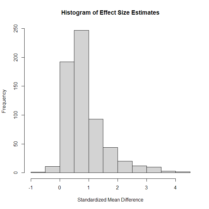
Figure 1.
The most important observation for this blog post is that there are hardly any effect sizes below zero. To understand why this is important, it is important to understand the meaning of the sign of an effect size. In an original study, the sign has no meaning. For example, the height differences between people with XX and XY chromosomes can be positive or negative depending on the coding of XX as 0 or 1 and XY as 1 or 0, respectively.
For a meta-analysis, however, the sign becomes meaningful. In a competently conducted meta-analysis, the sign reflects the substantive hypothesis of a study. If mortality salience is coded as 1 against a control condition coded as 0, and the theory predicted an increase in a dependent variable, a positive sign implies that the result was consistent with the prediction. If the prediction implies a decrease in the DV, a negative sign is consistent with the theory, and the sign has to be reversed. Thus, if researchers mostly make correct predictions about the direction of an effect, we would expect mostly positive signs. Sampling error can still produce negative means in studies, even if the true effect is in the predicted direction, but how often that happens depends on the strength of the effect.
Now we are in the position to make sense of Figure 1. Only 2% of the effect size estimates. There are two possible explanations for this finding. Either TMT studies mostly produce positive results because most studies have true effects or there is selection bias and results that contradict theoretical predictions are not published (a third option would be coding mistakes, where coders code all results as positive and ignore substantive hypotheses).
What happens when these data are analyzed with bias-correction models? It depends on the model. The PET/PEESE model regresses effect sizes on the sampling error under the assumption that all studies have a common effect size and that larger samples are less biased.
The reanalysis that produced Figure 2 reproduced the published estimate of -.114 standard deviations. Thus, even though there are hardly any negative results in the data, the average study is supposed to have made a prediction in the wrong direction because that is what a negative mean means. An analysis that removed the 10% largest effect sizes, produced a positive estimate of .29 standard deviations. It is interesting that removing strong results increases the average. This shows that the results depend on assumptions about the amount of bias for different effect size estimates. Here the largest effect size estimates come also from the smallest studies (N < 10).
The point estimate of .29 should not be confused with the true effect size in each study. After removing sampling error, there is still considerable variability in the effect size estimates that can be quantified with the standard deviation, assuming a normal distribution. The estimate is tau = .40. This also makes it possible to create a prediction interval – a confidence interval for the hypothetical population effect sizes . To get a 95%CI we roughly multiply tau by 2 and get a range of values around the point estimate from .29 – ,80 to .29 + .80. Thus, any particular TMT study could have an effect size anywhere from -.51 to + 1.09. In terms of Cohen’s classification of effect sizes the effect sizes range from a moderate negative effect size to a strong positive effect size. In other words, the data are not telling us anything that we did not know before we ran the analysis. Terror Management effects may sometimes emerge as predicted, sometimes with surprising opposite effects, and sometimes have no notable effects, and we do not know which manipulation produces which effect.
The problem in the published article and many other meta-analysis is that the heterogeneity in effect sizes after taking random sampling error was ignored. The point estimate is only needed to center the prediction interval. The real information is the wide range of possible population effect sizes that are consistent with the model’s assumptions and the data. Every outcome except large negative effect sizes is possible.
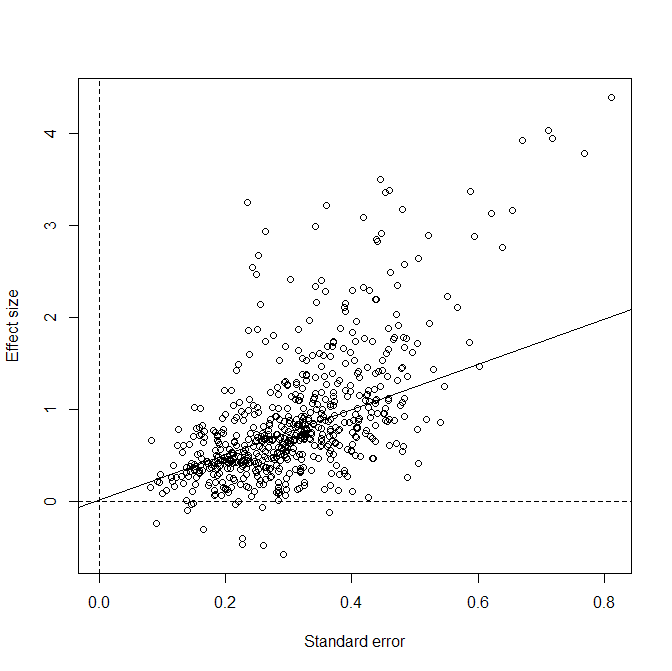
Regression models have many limitations and even the developer of this approach has warned against the use of this model for highly heterogenous data (Stanley, 2017). A model that is more suitable for heterogeneous data is the weight-function selection model (Vevea & Woods, 2005). However, this model requires assumptions about selection bias. Chen et al. fitted a model that assumes different selection bias for significant negative results and non-significant results. Importantly, their model assumed the same amount of selection bias for negative non-significant results and positive significant results. This specification is important because Figure 1 shows that there are few negative effect sizes. A better way to see the problem here is to convert effect sizes and sampling error into z-values (z = effect size / standard error) to distinguish between non-significant (z < 1.96) and significant ones.
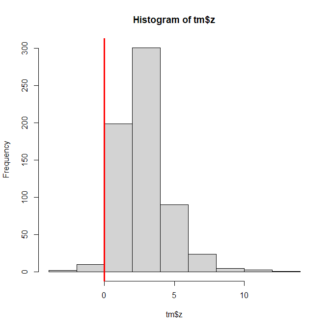
Figure 3 shows clearly that there is selection against negative results. Sampling error alone cannot explain the drop in effect size estimates from just above zero to just below zero.
The published article reports an estimated average effect size of .36. The model also estimated that only 26% of non-significant results were included in the meta-analysis. In other words, 74% were missing due to to publication bias. Finally, the model estimated that the population effect sizes had high heterogeneity, tau = .71. This leads to a very wide prediction interval around the point estimate of .36 ranging from .36 – 2*.71 to .36 + 2 * .71, which is -1.01 to 1.73. In other words, the model does not even exclude strong negative effect sizes as possible outcomes.
However, this model is misspecified because it ignores that selection against negative non-significant results is stronger than selection against non-significant positive results. I therefore ran the model again with an additional step at p = .5 (one-sided) that separates positive from negative results.. Consistent with the pattern in Figure 3, the model shows stronger selection against negative results (weight = .01, selection 1-weight = 99%) than for nonsignificant positive results (weight = .30, selection bias 70%). This improved model, however, produced a negative estimated average effect size of -.34. It also further increased the estimate of heterogeneity to tau = .96.
To understand this behavior of the model (I am more of a model analyst than a psycho-analyst), we need to understand the model’s assumption about the distribution of the unobserved population effect sizes. The model assumes an unobserved normal distribution, but the data are a truncated distribution at zero with no meaningful negative values. The model therefore fits the positive range of a normal distribution to the observed positive values. If this distribution is very wide, the normal has a large standard deviation and the model extrapolates it into the negative range. This leads to the wide prediction interval ranging from -1.34 to 2.58. Importantly, the negative range is entirely based on distribution assumption of the model . Changing the distribution assumption would change the results.
So, we have to think about the distribution assumption. When studies are more or less identical, there may be some extra variation in population effect sizes aside from sampling error. This variance can be approximated with a normal distribution (Hedges & Vevea, 1996). But when the set of studies has effect sizes ranging from 0 to 2, this is no longer plausible. If the average effect size is small and heterogeneity is large, a normal distribution implies that many substantive hypotheses have the wrong sign, but that is not really plausible. Many studies may have no real effect or really small ones, but it is harder to argue and to believe that researchers often get the sign of an effect wrong, especially when there is a real effect. Reminding people of their death makes them afraid is a reasonable hypothesis, and it would be surprising if studies show the opposite result.
In short, the weight-function model is not wrong, but applying a model that assumes a normal distribution to highly heterogeneous data is wrong. The model predicts many negative results that do not match any observed results. It could be selection bias, but it could also be a false distribution assumption. What to do?
A reasonable approach to make sense of results from the selection model is to focus on the positive side of the distribution. With normal distributions it is easy to get other statistics like the mean of only positive results (or any other subset of studies). We can therefore ignore studies with false substantive hypotheses and focus on studies where researchers made correct predictions about the sign of an effect (H1 is true).
With a mean of -.34 and tau = .956, we get a conditional mean for studies in which H1 is true of .65 standard deviations (a medium to large effect size) with tau of .52. As the lower bound is zero, we only need the upper bound and get .65 + 1.96 * .52 which is 1.67. This would suggest that many studies have strong effect sizes, which seems to contradict the estimated center of the distribution at -.34. This shows how meaningless these point estimates are when heterogeneity is large.
Unfortunately for terror management researchers the truncated moments are not going to rescue their literature because they are hypothetical. The reason is that we are conditioning on an unknown parameter, namely the condition that the hypothesis was true, but for any particular study we do not know whether H1 is true or not. So, the correct way to formulate this result is “if you can identify a study design in which terror management theory makes the right prediction and you can get a fairly precise estimate of the true effect size, you can expect a moderate effect size estimate.
What the weight-function model does not provide is a bias-corrected estimate of the positive effect size estimates in the dataset. The mean of the full distribution includes negative results that were either removed or never obtained. The truncated moment estimate conditions on the unknown status of the null-hypothesis. One is likely too low and the other is likely to high, but neither is conceptually the estimate we want. The average population effect size positive studies that corrects for the selection of nonsignificant results.
To summarize, state of the art meta-analyses in psychology try to deal with the terror of publication bias, but fail to do so. The main reason is that the statistical models that are available do not match the data. They were designed for meta-analysis of close replications with small variation in true effect sizes. They were not intended to be used for meta-analyses of diverse paradigms with large heterogeneity. Other methods that were developed after the replication crisis like p-curve and p-uniform have the same limitation. They work when heterogeneity is small, but they do not work for meta-analyses of diverse studies that are only loosely related by a common hypothesis.
Z-Curve to the Rescue
The quote “Insanity is trying the same thing and expecting a different result” has been attributed to Einstein. Even if that attribution is false, the insight is right. The problem with meta-analytic models is that they try to estimate a single number. This makes sense when the goal is estimation of a single population effect size, but not when every study has a different population effect size.
When we have a heterogenous literature, we need to face heterogeneity head on, and not hide it in some test that is reported and ignored. There is also heterogeneity around the estimate, p < .05. We need to see how much heterogeneity there. But to do that, we first need a model that can deal with heterogeneity without making unrealistic assumptions about the distribution of population effect sizes.
With a fresh look at the problem, we can look to other research areas that have addressed the problem of heterogeneity in effect sizes and large uncertainty about effect sizes of a specific result. Genomics tests millions of DNA segments (SNPs) and tries to find a few segments that show promising results. The goal here is to find the needles in the hey stack rather than averaging across millions of segments that have no relationship with a phenotype. As selection for the strongest observed effects leads to inflated estimates, models are needed to correct for this inflation. However, these corrected estimates are still tight to actual observed results rather than claims about some unobserved distribution of effect sizes. That makes it possible to identify specific segments in the observed data with promising results.
The same logic can be applied to meta-analysis. The goal is no longer to make claims like “the average population effect size is zero” or “the range of plausible effect sizes ranges from -1 to 1.” the goal is now to say “these studies show convincing evidence with meaningful effect sizes.”
One statistical model that can be used to answer this question is zurve (Brunner & Schimmack, 2020; Bartos & Schimmack, 2022). With a few modifications, z-curve can be used for directional meta-analysis where the sign of an effect matters. Rather than fitting z-curve to absolute z-values that ignore the sign and using folded normal components, z-curve can use truncated z-values and truncated normal components. When the model is fitted to only significant results, the difference is minor. More importantly, z-curve estimates of power can also be used to compute bias-corrected effect sizes (Efron, 2005). The reason is that power is a function of effect size and sampling error, so we can use the inverse normal to convert power into a corrected z-value and then multiply it with the sampling error to get a bias corrected effect size. The main challenge is to estimate the sampling error for unobserved non-significant results because their sample sizes are unknown. A simple approach is to use the sampling errors of the just significant results as an approximation. A weighted average of these estimates is the estimate of the true average effect size for the population of studies with positive results before selection for significance. Negative results that are observed are discarded.
Figure 4 shows the results of a simulation study in which the true average power before selection is known. The simulation modeled a beta distribution and graded selection bias. This is important because the weight-function model does well when its assumptions are met. The problem is that the assumptions are are untestable and often questionable. For example, we can simulate a literature with a mean of zero and tau of .4, but this simulation implies that a theories predictions are no better than a coin flip. Once researchers make better predictions, the normal assumption no longer holds.
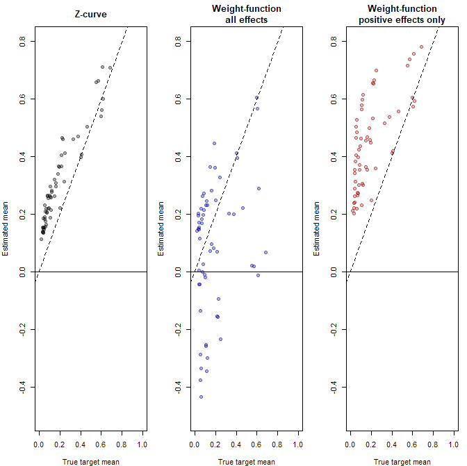
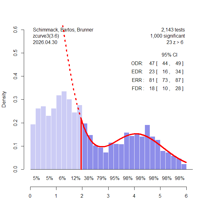
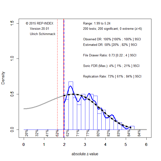
While z-curve estimates are not perfect, they are conceptually meaningful and closer to the truth than either of the weight-function model’s estimates. We can now apply the model to the TMT data, excluding the few (2%) negative estimates.
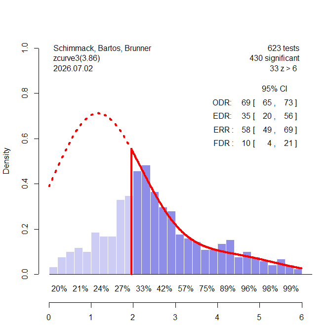
The z-curve shows clear evidence of selection bias (the red dotted line is above the light purple bars of the nonsignificant results. However, the EDR estimate of 35% suggests that studies have on average 33% power to produce a significant result. Moreover, an EDR of 33% implies that no more than 10% of the significant results can be false positive results. Even the lower limit of the EDR confidence interval, 20%, allows for only 20% false positive results. This would suggest that many studies, especially significant ones, produced evidence for a true hypotheses with an effect size in the right direction. We can now also quantify the typical effect size. The overall effect size estimate is .63, 95%CI [.46 to .68]. Moreover, we can quantify the average for different ranges of z-values. The average increases from .40 for z-values between 0 and 0.5 to effect sizes greater than 1 for z-values greater than 4.
This finding is surprising, to say the least, because typical effect sizes in psychology are around d = .4 and rarely greater than 1. Before TMT researchers start celebrating, we have to reconcile these findings with the z-curve analysis published in the TMT article.
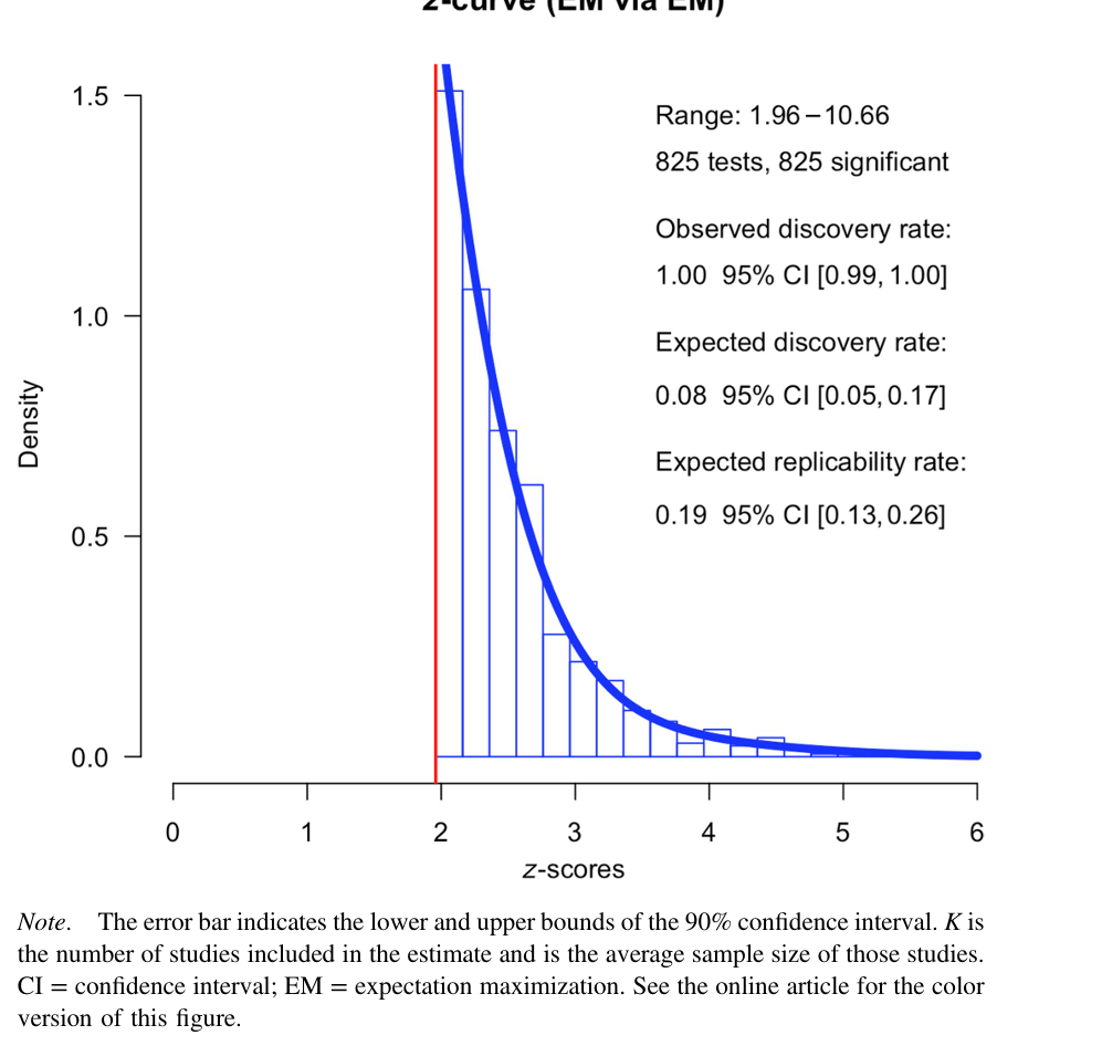
The z-curve looks notably different in that it does not have a long tail of high z-values. As a result, the EDR estimate is much lower, .08, and the 95% confidence interval includes alpha, 5% to 17%. This implies that there is no t enough evidence to reject the null-hypothesis that all significant results were obtained without a real effect, average effect size: zero, even for z-values greater than 4. So what is it? Is the average effect size close to zero or greater than 1?
To understand the different results, it is important to know that the published z-curve used a different coding of studies than the effect size meta-analysis. I fitted z-curve to these z-values and computed effect size and sampling error estimates from the z-values and degrees of freedom, assuming between-subject designs with equal cell sizes.

The plot is scaled to show the full distribution in the range of non-significant results. The model estimates reproduce the published results. The EDR is 7%, 95%CI = [5%, 17%]. The plot also shows local power for z-values from 0 to 3 stays low. Studies with z-values greater than 4 have acceptable local power but contrary to the previous z-curve, there are hardly any studies. This published z-curve produces dramatically different average effect size estimate, .12 95%CI = .02 to .19. The results also imply much lower heterogeneity because there are hardly any studies with strong evidence (z > 4) and large effect sizes.
Applying the weight-function selection model produces roughly the same results. The average effect size estimate is d = .17, and heterogeneity is small, tau = .17. Now the PET regression result also agrees, intercept = .05, tau = .19.
In conclusion, careful examination of this meta-analysis shows several problems. First, the data were coded inconsistently and different models were given different data. As it turns out, the effect size coding was wrong because F-values were coded as t-values, which dramatically inflates effect size estimates. Second, inconsistent results focused on the point estimate of models, but the point estimate is irrelevant when data are highly heterogenous (due to coding mistakes). Properly interpreted, all models suggest high heterogeneity that allows for large effect sizes among positive results. However, when the data are properly coded, the results show weak evidence that any study produced real effects, a high false positive risk, a small average effect size and small heterogeneity. These results change the final conclusion in the article.
“Given the conflicting findings that emerged across tools and the inherent trade-offs associated with each tool, we caution researchers against drawing firm conclusions about the evidential value of literature through any single analytic tool.”
Correction: The results are consistent and show that most studies provide no evidence for an effect because most effect sizes are small and studies had low power to detect or estimate these effects.
“PET-PEESE can underestimate the effect size when there is publication bias and when p-hacking is present (Carter et al., 2019), which are two conditions likely affecting the literature.”
Here bad research practices are used as an excuse to dismiss the most negative result without mentioning the real problem There is no “effect size.: there is only an average effect size and regression models still allow estimation of heterogeneity that was large in the data the authors used. Even a negative average can be consistent with many true positive effects when heterogeneity is large.
Z-curve can be a powerful tool for inferring the overall composite z-score distribution of a heterogeneous literature. However, unlike the other analyses included in this study, z-curve has not been as thoroughly evaluated by independent researchers so the statistical properties for its power estimates remain under explored. Furthermore, its power estimates are subject to the usual theoretical objections to estimating power from a fixed sample of data (for a recent commentary, see Pek et al., 2022).
This statement ignores that z-curve has been thoroughly evaluated by extensive simulations studies that have been reproduced by the editorial team during an open peer review process. The same cannot be said about the other methods that have not been vetted as rigorously or failed to do well in some conditions (Carter et al., 2019). The reference to Pek is also misleading which has been addressed in several rebuttals to this unfounded claim (Schimmack & Soto, 2026; Soto & Schimmack,2026) with no rejoinder by Pek.
The higher conditional power estimate therefore suggests some evidential value in published studies that yielded significant findings.
The authors are referring to the ERR estimate of 22% [16% , 37%]. Suddenly Pek’s criticism of z-curve is no longer relevant. More importantly, this finding implies that an exact replication of a study with a significant result has a 22% chance of a successful replication outcome. This is abysmal and one of the lowest ever found, not a cause for optimism. Surely reminders of mortality will sometimes have an effect on something, but a research program that uses different designs with an average power of 22% will not be able to identify when a manipulation works or when it is just a chance finding. In fact, the upper limit of the DR estimate is 100%. Thus, these weak studies fail to reject the hypothesis that all studies are pure noise.
“The selection models provide evidence for a small effect consistent with the MS hypothesis… We suggest that the average effect of the literature may be within the range estimated by the selection models and WAAP-WLS (i.e., r is around .18), although this average may have resulted from a mix of effects, many of which are higher than .18, and many of which are lower than .18.
The average estimate is too high once we correct for the coding mistakes. The real effect size is half of this (d = r / 2), and heterogeneity is small. This is the most conesquences conclusoin. Rather than having evidence of a wide range of positive effect sizes, we have evidence that most effect sizes are small and too small to study with the typical sample sizes of this literature.
We encourage future preregistered replications of the MS hypothesis to use smaller es
timates of effect size (i.e., r = .18).
This inflated effect size estimate will only lead to a replication failure. Given the weak evidence in this literature, it may be better to start a new credible research program about coping with awareness of one’s own mortality than to invest more resources into this failed paradigm with questionable manipulations and dependent variables.
Though on their face the liberal and conservative interpretations feel contradictory, some observations are uncontroversial. The first observation is that the TMT literature consists of highly heterogenous.
Even this conclusion turns out to be false when the proper data are analyzed. Heterogeneity was caused by coding mistakes and practically vanishes when the correct data coded by the authors were analyzed. The authors did not notice that their data were inconsistent, even though a simple comparison of the z-values would have shown the discrepancy. It is natural for humans to make errors, but errors also reveal something about the person who committed the error. In this case, it reveals a lack of understanding of the methods, their assumptions, and why they may produce inconsistent results. Here inconsistency was attributed to properties of the models when the real source were inconsistent data. In the future, meta-analysts should not just report inconsistencies, but also try to explain them. That requires understanding of the tools that they use.
For our entire universe of studies, heterogeneity is estimated at τ = .72 under the selection models, which means that for the estimate of g = 0.36 (r = .18) for the entire literature from the selection models, 95% of the effects underlying studies of MS hypothesis, assuming a normal distribution of g, fall between g = −1.05 and 1.77 (or r = −.47 and .66); an extremely wide range of possible effect sizes arising from differences in study design.
The problem with this wide range of population effect sizes is the assumption of a normal distribution. Even if no negative results are observed, the assumption leads to the conclusion that negative effects were obtained but suppressed. But researchers are flexible and it is more likely that they would change the prediction in the direction of a significant result (Kerr, 1998). Thus, it is highly likely that the predicted negative results are phantom studies that do not exist. These predicted effect sizes surely do not correspond to the positive estimates in the dataset.
With these observations in mind, we conclude that there must be some nonzero underlying effects in the studies we examined.
That sounds more reassuring than it is. We have over 800 results and some of these are not false positives. Great, now what? We do not know which of these results are true or false positives. So, we haven’t really learned anything about mortality awareness from this meta-analysis. Fortunately, the analysis of the data without the coding mistake is more conclusive. Terror management research is an example of a pathological science. Researchers conduct studies but never learn form their data because they find a way to keep their theory alive. A proper analysis shows that we can put this literature to rest. That is ok. The history of science is filled with failures. It is also filled with examples where researchers are unable to learn from their errors. However, science moves on and experimental social psychology with little priming manipulations will be a little footnote in the history books.
P.S. And z-curve works and can now also estimate effect sizes.