Tag Archives: Science

Distinguishing Questionable Research Practices from Publication Bias

It is well-known that scientific journals favor statistically significant results (Sterling, 1959). This phenomenon is known as publication bias. Publication bias can be easily detected by comparing the observed statistical power of studies with the success rate in journals. Success rates of 90% or more would only be expected if most theoretical predictions are true and empirical studies have over 90% statistical power to produce significant results. Estimates of statistical power range from 20% to 50% (Button et al., 2015, Cohen, 1962). It follows that for every published significant result an unknown number of non-significant results has occurred that remained unpublished. These results linger in researchers proverbial file-drawer or more literally in unpublished data sets on researchers’ computers.

The selection of significant results also creates an incentive for researchers to produce significant results. In rare cases, researchers simply fabricate data to produce significant results. However, scientific fraud is rare. A more serious threat to the integrity of science is the use of questionable research practices. Questionable research practices are all research activities that create a systematic bias in empirical results. Although systematic bias can produce too many or too few significant results, the incentive to publish significant results suggests that questionable research practices are typically used to produce significant results.

In sum, publication bias and questionable research practices contribute to an inflated success rate in scientific journals. So far, it has been difficult to examine the prevalence of questionable research practices in science. One reason is that publication bias and questionable research practices are conceptually overlapping. For example, a research article may report the results of a 2 x 2 x 2 ANOVA or a regression analysis with 5 predictor variables. The article may only report the significant results and omit detailed reporting of the non-significant results. For example, researchers may state that none of the gender effects were significant and not report the results for main effects or interaction with gender. I classify these cases as publication bias because each result tests a different hypothesis., even if the statistical tests are not independent.

Questionable research practices are practices that change the probability of obtaining a specific significant result. An example would be a study with multiple outcome measures that would support the same theoretical hypothesis. For example, a clinical trial of an anti-depressant might include several depression measures. In this case, a researcher can increase the chances of a significant result by conducting tests for each measure. Other questionable research practices would be optional stopping once a significant result is obtained, selective deletion of cases based on the results after deletion. A common consequence of these questionable practices is that they will produce results that meet the significance criterion, but deviate from the distribution that is expected simply on the basis of random sampling error.

A number of articles have tried to examine the prevalence of questionable research practices by comparing the frequency of p-values above and below the typical criterion of statistical significance, namely a p-value less than .05. The logic is that random error would produce a nearly equal amount of p-values just above .05 (e.g., p = .06) and below .05 (e.g., p = .04). According to this logic, questionable research practices are present, if there are more p-values just below the criterion than p-values just above the criterion (Masicampo & Lalande, 2012).

Daniel Lakens has pointed out some problems with this approach. The most crucial problem is that publication bias alone is sufficient to predict a lower frequency of p-values below the significance criterion. After all, these p-values imply a non-significant result and non-significant results are subject to publication bias. The only reason why p-values of .06 are reported with higher frequency than p-values of .11 is that p-values between .05 and .10 are sometimes reported as marginally significant evidence for a hypothesis. Another problem is that many p-values of .04 are not reported as p = .04, but are reported as p < .05. Thus, the distribution of p-values close to the criterion value provides unreliable information about the prevalence of questionable research practices.

In this blog post, I introduce an alternative approach to the detection of questionable research practices that produce just significant results. Questionable research practices and publication bias have different effects on the distribution of p-values (or corresponding measures of strength of evidence). Whereas publication bias will produce a distribution that is consistent with the average power of studies, questionable research practice will produce an abnormal distribution with a peak just below the significance criterion. In other words, questionable research practices produce a distribution with too few non-significant results and too few highly significant results.

I illustrate this test of questionable research practices with post-hoc-power analysis of three journals. One journal shows neither signs of publication bias, nor significant signs of questionable research practices. The second journal shows clear evidence of publication bias, but no evidence of questionable research practices. The third journal illustrates the influence of publication bias and questionable research practices.

Example 1: A Relatively Unbiased Z-Curve

The first example is based on results published during the years 2010-2014 in the Journal of Experimental Psychology: Learning, Memory, and Cognition. A text-mining program searched all articles for publications of F-tests, t-tests, correlation coefficients, regression coefficients, odds-ratios, confidence intervals, and z-tests. Due to the inconsistent and imprecise reporting of p-values (p = .02 or p < .05), p-values were not used. All statistical tests were converted into absolute z-scores.

The program found 14,800 tests. 8,423 tests were in the critical interval between z = 2 and z = 6 that is used for estimation of 4 non-centrality parameters and 4 weights that are used to model the distribution of z-values between 2 and 6 and to estimate the distribution in the range from 0 to 2. Z-values greater than 6 are not used because they correspond to Power close to 1. 11% of all tests fall into this region of z-scores that are not shown.

PHP-Curve JEP-LMC
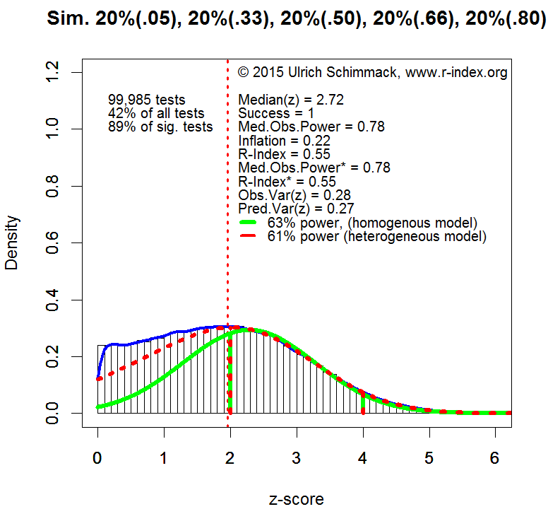
The histogram and the blue density distribution show the observed data. The green curve shows the predicted distribution based on the post-hoc power analysis. Post-hoc power analysis suggests that the average power of significant results is 67%. Power for all statistical tests is estimated to be 58% (including 11% of z-scores greater than 6, power is .58*.89 + .11 = 63%). More important is the predicted distribution of z-scores. The predicted distribution on the left side of the criterion value matches the observed distribution rather well. This shows that there are not a lot of missing non-significant results. In other words, there does not appear to be a file-drawer of studies with non-significant results. There is also only a very small blip in the observed data just at the level of statistical significance. The close match between the observed and predicted distributions suggests that results in this journal are relatively free of systematic bias due to publication bias or questionable research practices.

Example 2: A Z-Curve with Publication Bias

The second example is based on results published in the Attitudes & Social Cognition Section of the Journal of Personality and Social Psychology. The text-mining program retrieved 5,919 tests from articles published between 2010 and 2014. 3,584 tests provided z-scores in the range from 2 to 6 that is being used for model fitting.

PHP-Curve JPSP-ASC

The average power of significant results in JPSP-ASC is 55%. This is significantly less than the average power in JEP-LMC, which was used for the first example. The estimated power for all statistical tests, including those in the estimated file drawer, is 35%. More important is the estimated distribution of z-values. On the right side of the significance criterion the estimated curve shows relatively close fit to the observed distribution. This finding shows that random sampling error alone is sufficient to explain the observed distribution. However, on the left side of the distribution, the observed z-scores drop off steeply. This drop is consistent with the effect of publication bias that researchers do not report all non-significant results. There is only a slight hint that questionable research practices are also present because observed z-scores just above the criterion value are a bit more frequent than the model predicts. However, this discrepancy is not conclusive because the model could increase the file drawer, which would produce a steeper slope. The most important characteristic of this z-curve is the steep cliff on the left side of the criterion value and the gentle slope on the right side of the criterion value.

Example 3: A Z-Curve with Questionable Research Practices.

Example 3 uses results published in the journal Aggressive Behavior during the years 2010 to 2014. The text mining program found 1,429 results and 863 z-scores in the range from 2 to 6 that were used for the post-hoc-power analysis.

PHP-Curve for AggressiveBeh 2010-14


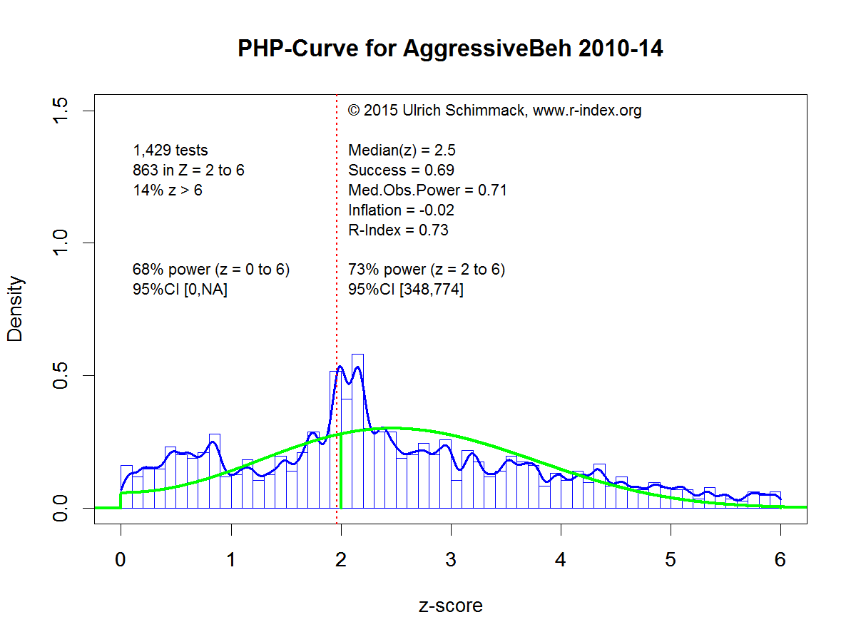
The average power for significant results in the range from 2 to 6 is 73%, which is similar to the power estimate in the first example. The power estimate that includes non-significant results is 68%. The power estimate is similar because there is no evidence of a file drawer with many underpowered studies. In fact, there are more observed non-significant results than predicted non-significant results, especially for z-scores close to zero. This outcome shows some problems of estimating the frequency of non-significant results based on the distribution of significant results. More important, the graph shows a cluster of z-scores just above and below the significance criterion. The step cliff to the left of the criterion might suggest publication bias, but the whole distribution does not show evidence of publication bias. Moreover, the steep cliff on the right side of the cluster cannot be explained with publication bias. Only questionable research practices can produce this cliff because publication bias relies on random sampling error which leads to a gentle slope of z-scores as shown in the second example.

Prevalence of Questionable Research Practices

The examples suggest that the distribution of z-scores can be used to distinguish publication bias and questionable research practices. Based on this approach, the prevalence of questionable research practices would be rare. The journal Aggressive Behavior is exceptional. Most journals show a pattern similar to Example 2, with varying sizes of the file drawer. However, this does not mean that questionable research practices are rare because it is most likely that the pattern observed in Example 2 is a combination of questionable research practices and publication bias. As shown in Example 2, the typical power of statistical tests that produce a significant result is about 60%. However, researchers do not know which experiments will produce significant results. Slight modifications in experimental procedures, so-called hidden moderators, can easily change an experiment with 60% power into an experiment with 30% power. Thus, the probability of obtaining a significant result in a replication study is less than the nominal power of 60% that is implied by post-hoc-power analysis. With only 30% to 60% power, researchers will frequently encounter results that fail to produce an expected significant result. In this case, researchers have two choices to avoid reporting a non-significant result. They can put the study in the file-drawer or they can try to salvage the study with the help of questionable research practices. It is likely that researchers will do both and that the course of action depends on the results. If the data show a trend in the right direction, questionable research practices seem an attractive alternative. If the data show a trend in the opposite direction, it is more likely that the study will be terminated and the results remain unreported.

Simons et al. (2011) conducted some simulation studies and found that even extreme use of multiple questionable research practices (p-hacking) will produce a significant result in at most 60% of cases, when the null-hypothesis is true. If such extreme use of questionable research practices were widespread, z-curve would produce corrected power estimates well-below 50%. There is no evidence that extreme use of questionable research practices is prevalent. In contrast, there is strong evidence that researchers conduct many more studies than they actually report and that many of these studies have a low probability of success.

Implications of File-Drawers for Science

First, it is clear that researchers could be more effective if they would use existing resources more effectively. An fMRI study with 20 participants costs about $10,000. Conducting a study that costs $10,000 that has only a 50% probability of producing a significant result is wasteful and should not be funded by taxpayers. Just publishing the non-significant result does not fix this problem because a non-significant result in a study with 50% power is inconclusive. Even if the predicted effect exists, one would expect a non-significant result in ever second study.   Instead of wasting $10,000 on studies with 50% power, researchers should invest $20,000 in studies with higher power (unfortunately, power does not increase proportional to resources). With the same research budget, more money would contribute to results that are being published. Thus, without spending more money, science could progress faster.

Second, higher powered studies make non-significant results more relevant. If a study had 80% power, there is only a 20% chance to get a non-significant result if an effect is present. If a study had 95% power, the chance of a non-significant result would be just as low as the chance of a false positive result. In this case, it is noteworthy that a theoretical prediction was not confirmed. In a set of high-powered studies, a post-hoc power analysis would show a bimodal distribution with clusters of z-scores around 0 for true null-hypothesis and a cluster of z-scores of 3 or higher for clear effects. Type-I and Type-II errors would be rare.

Third, Example 3 shows that the use of questionable research practices becomes detectable in the absence of a file drawer and that it would be harder to publish results that were obtained with questionable research practices.

Finally, the ability to estimate the size of file-drawers may encourage researchers to plan studies more carefully and to invest more resources into studies to keep their file drawers small because a large file-drawer may harm reputation or decrease funding.

In conclusion, post-hoc power analysis of large sets of data can be used to estimate the size of the file drawer based on the distribution of z-scores on the right side of a significance criterion. As file-drawers harm science, this tool can be used as an incentive to conduct studies that produce credible results and thus reducing the need for dishonest research practices. In this regard, the use of post-hoc power analysis complements other efforts towards open science such as preregistration and data sharing.

REPLICABILITY RANKING OF 26 PSYCHOLOGY JOURNALS

THEORETICAL BACKGROUND

Neyman & Pearson (1933) developed the theory of type-I and type-II errors in statistical hypothesis testing.

A type-I error is defined as the probability of rejecting the null-hypothesis (i.e., the effect size is zero) when the null-hypothesis is true.

A type-II error is defined as the probability of failing to reject the null-hypothesis when the null-hypothesis is false (i.e., there is an effect).

A common application of statistics is to provide empirical evidence for a theoretically predicted relationship between two variables (cause-effect or covariation). The results of an empirical study can produce two outcomes. Either the result is statistically significant or it is not statistically significant. Statistically significant results are interpreted as support for a theoretically predicted effect.

Statistically non-significant results are difficult to interpret because the prediction may be false (the null-hypothesis is true) or a type-II error occurred (the theoretical prediction is correct, but the results fail to provide sufficient evidence for it).

To avoid type-II errors, researchers can design studies that reduce the type-II error probability. The probability of avoiding a type-II error when a predicted effect exists is called power. It could also be called the probability of success because a significant result can be used to provide empirical support for a hypothesis.

Ideally researchers would want to maximize power to avoid type-II errors. However, powerful studies require more resources. Thus, researchers face a trade-off between the allocation of resources and their probability to obtain a statistically significant result.

Jacob Cohen dedicated a large portion of his career to help researchers with the task of planning studies that can produce a successful result, if the theoretical prediction is true. He suggested that researchers should plan studies to have 80% power. With 80% power, the type-II error rate is still 20%, which means that 1 out of 5 studies in which a theoretical prediction is true would fail to produce a statistically significant result.

Cohen (1962) examined the typical effect sizes in psychology and found that the typical effect size for the mean difference between two groups (e.g., men and women or experimental vs. control group) is about half-of a standard deviation. The standardized effect size measure is called Cohen’s d in his honor. Based on his review of the literature, Cohen suggested that an effect size of d = .2 is small, d = .5 moderate, and d = .8. Importantly, a statistically small effect size can have huge practical importance. Thus, these labels should not be used to make claims about the practical importance of effects. The main purpose of these labels is that researchers can better plan their studies. If researchers expect a large effect (d = .8), they need a relatively small sample to have high power. If researchers expect a small effect (d = .2), they need a large sample to have high power.   Cohen (1992) provided information about effect sizes and sample sizes for different statistical tests (chi-square, correlation, ANOVA, etc.).

Cohen (1962) conducted a meta-analysis of studies published in a prominent psychology journal. Based on the typical effect size and sample size in these studies, Cohen estimated that the average power in studies is about 60%. Importantly, this also means that the typical power to detect small effects is less than 60%. Thus, many studies in psychology have low power and a high type-II error probability. As a result, one would expect that journals often report that studies failed to support theoretical predictions. However, the success rate in psychological journals is over 90% (Sterling, 1959; Sterling, Rosenbaum, & Weinkam, 1995). There are two explanations for discrepancies between the reported success rate and the success probability (power) in psychology. One explanation is that researchers conduct multiple studies and only report successful studies. The other studies remain unreported in a proverbial file-drawer (Rosenthal, 1979). The other explanation is that researchers use questionable research practices to produce significant results in a study (John, Loewenstein, & Prelec, 2012). Both practices have undesirable consequences for the credibility and replicability of published results in psychological journals.

A simple solution to the problem would be to increase the statistical power of studies. If the power of psychological studies in psychology were over 90%, a success rate of 90% would be justified by the actual probability of obtaining significant results. However, meta-analysis and method articles have repeatedly pointed out that psychologists do not consider statistical power in the planning of their studies and that studies continue to be underpowered (Maxwell, 2004; Schimmack, 2012; Sedlmeier & Giegerenzer, 1989).

One reason for the persistent neglect of power could be that researchers have no awareness of the typical power of their studies. This could happen because observed power in a single study is an imperfect indicator of true power (Yuan & Maxwell, 2005). If a study produced a significant result, the observed power is at least 50%, even if the true power is only 30%. Even if the null-hypothesis is true, and researchers publish only type-I errors, observed power is dramatically inflated to 62%, when the true power is only 5% (the type-I error rate). Thus, Cohen’s estimate of 60% power is not very reassuring.

Over the past years, Schimmack and Brunner have developed a method to estimate power for sets of studies with heterogeneous designs, sample sizes, and effect sizes. A technical report is in preparation. The basic logic of this approach is to convert results of all statistical tests into z-scores using the one-tailed p-value of a statistical test.  The z-scores provide a common metric for observed statistical results. The standard normal distribution predicts the distribution of observed z-scores for a fixed value of true power.   However, for heterogeneous sets of studies the distribution of z-scores is a mixture of standard normal distributions with different weights attached to various power values. To illustrate this method, the histograms of z-scores below show simulated data with 10,000 observations with varying levels of true power: 20% null-hypotheses being true (5% power), 20% of studies with 33% power, 20% of studies with 50% power, 20% of studies with 66% power, and 20% of studies with 80% power.

RepRankSimulation

The plot shows the distribution of absolute z-scores (there are no negative effect sizes). The plot is limited to z-scores below 6 (N = 99,985 out of 10,000). Z-scores above 6 standard deviations from zero are extremely unlikely to occur by chance. Even with a conservative estimate of effect size (lower bound of 95% confidence interval), observed power is well above 99%. Moreover, quantum physics uses Z = 5 as a criterion to claim success (e.g., discovery of Higgs-Boson Particle). Thus, Z-scores above 6 can be expected to be highly replicable effects.

Z-scores below 1.96 (the vertical dotted red line) are not significant for the standard criterion of (p < .05, two-tailed). These values are excluded from the calculation of power because these results are either not reported or not interpreted as evidence for an effect. It is still important to realize that true power of all experiments would be lower if these studies were included because many of the non-significant results are produced by studies with 33% power. These non-significant results create two problems. Researchers wasted resources on studies with inconclusive results and readers may be tempted to misinterpret these results as evidence that an effect does not exist (e.g., a drug does not have side effects) when an effect is actually present. In practice, it is difficult to estimate power for non-significant results because the size of the file-drawer is difficult to estimate.

It is possible to estimate power for any range of z-scores, but I prefer the range of z-scores from 2 (just significant) to 4. A z-score of 4 has a 95% confidence interval that ranges from 2 to 6. Thus, even if the observed effect size is inflated, there is still a high chance that a replication study would produce a significant result (Z > 2). Thus, all z-scores greater than 4 can be treated as cases with 100% power. The plot also shows that conclusions are unlikely to change by using a wider range of z-scores because most of the significant results correspond to z-scores between 2 and 4 (89%).

The typical power of studies is estimated based on the distribution of z-scores between 2 and 4. A steep decrease from left to right suggests low power. A steep increase suggests high power. If the peak (mode) of the distribution were centered over Z = 2.8, the data would conform to Cohen’s recommendation to have 80% power.

Using the known distribution of power to estimate power in the critical range gives a power estimate of 61%. A simpler model that assumes a fixed power value for all studies produces a slightly inflated estimate of 63%. Although the heterogeneous model is correct, the plot shows that the homogeneous model provides a reasonable approximation when estimates are limited to a narrow range of Z-scores. Thus, I used the homogeneous model to estimate the typical power of significant results reported in psychological journals.

DATA

The results presented below are based on an ongoing project that examines power in psychological journals (see results section for the list of journals included so far). The set of journals does not include journals that primarily publish reviews and meta-analysis or clinical and applied journals. The data analysis is limited to the years from 2009 to 2015 to provide information about the typical power in contemporary research. Results regarding historic trends will be reported in a forthcoming article.

I downloaded pdf files of all articles published in the selected journals and converted the pdf files to text files. I then extracted all t-tests and F-tests that were reported in the text of the results section searching for t(df) or F(df1,df2). All t and F statistics were converted into one-tailed p-values and then converted into z-scores.

RepRankAll

The plot above shows the results based on 218,698 t and F tests reported between 2009 and 2015 in the selected psychology journals. Unlike the simulated data, the plot shows a steep drop for z-scores just below the threshold of significance (z = 1.96). This drop is due to the tendency not to publish or report non-significant results. The heterogeneous model uses the distribution of non-significant results to estimate the size of the file-drawer (unpublished non-significant results). However, for the present purpose the size of the file-drawer is irrelevant because power is estimated only for significant results for Z-scores between 2 and 4.

The green line shows the best fitting estimate for the homogeneous model. The red curve shows fit of the heterogeneous model. The heterogeneous model is doing a much better job at fitting the long tail of highly significant results, but for the critical interval of z-scores between 2 and 4, the two models provide similar estimates of power (55% homogeneous & 53% heterogeneous model).   If the range is extended to z-scores between 2 and 6, power estimates diverge (82% homogenous, 61% heterogeneous). The plot indicates that the heterogeneous model fits the data better and that the 61% estimate is a better estimate of true power for significant results in this range. Thus, the results are in line with Cohen (1962) estimate that psychological studies average 60% power.

REPLICABILITY RANKING

The distribution of z-scores between 2 and 4 was used to estimate the average power separately for each journal. As power is the probability to obtain a significant result, this measure estimates the replicability of results published in a particular journal if researchers would reproduce the studies under identical conditions with the same sample size (exact replication). Thus, even though the selection criterion ensured that all tests produced a significant result (100% success rate), the replication rate is expected to be only about 50%, even if the replication studies successfully reproduce the conditions of the published studies. The table below shows the replicability ranking of the journals, the replicability score, and a grade. Journals are graded based on a scheme that is similar to grading schemes for undergraduate students (below 50 = F, 50-59 = E, 60-69 = D, 70-79 = C, 80-89 = B, 90+ = A).

ReplicabilityRanking

The average value in 2000-2014 is 57 (D+). The average value in 2015 is 58 (D+). The correlation for the values in 2010-2014 and those in 2015 is r = .66.   These findings show that the replicability scores are reliable and that journals differ systematically in the power of published studies.

LIMITATIONS

The main limitation of the method is that focuses on t and F-tests. The results might change when other statistics are included in the analysis. The next goal is to incorporate correlations and regression coefficients.

The second limitation is that the analysis does not discriminate between primary hypothesis tests and secondary analyses. For example, an article may find a significant main effect for gender, but the critical test is whether gender interacts with an experimental manipulation. It is possible that some journals have lower scores because they report more secondary analyses with lower power. To address this issue, it will be necessary to code articles in terms of the importance of statistical test.

The ranking for 2015 is based on the currently available data and may change when more data become available. Readers should also avoid interpreting small differences in replicability scores as these scores are likely to fluctuate. However, the strong correlation over time suggests that there are meaningful differences in the replicability and credibility of published results across journals.

CONCLUSION

This article provides objective information about the replicability of published findings in psychology journals. None of the journals reaches Cohen’s recommended level of 80% replicability. Average replicability is just about 50%. This finding is largely consistent with Cohen’s analysis of power over 50 years ago. The publication of the first replicability analysis by journal should provide an incentive to editors to increase the reputation of their journal by paying more attention to the quality of the published data. In this regard, it is noteworthy that replicability scores diverge from traditional indicators of journal prestige such as impact factors. Ideally, the impact of an empirical article should be aligned with the replicability of the empirical results. Thus, the replicability index may also help researchers to base their own research on credible results that are published in journals with a high replicability score and to avoid incredible results that are published in journals with a low replicability score. Ultimately, I can only hope that journals will start competing with each other for a top spot in the replicability rankings and as a by-product increase the replicability of published findings and the credibility of psychological science.

Using the R-index to detect questionable research practices in SSRI studies

Amna Shakil and Ulrich Schimmack

In 2008, Turner and colleagues (2008) examined the presence of publication bias in clinical trials of antidepressants. They found that out of 74 FDA-registered studies, 51% showed positive results. However, positive results were much more likely to be published, as 94% of the published results were positive. There were two reasons for the inflated percentage of positive results. First, negative results were not published. Second, negative results were published as positive results. Turner and colleagues’ (2008) results received a lot of attention and cast doubt on the effectiveness of anti-depressants.

A year after Turner and colleagues (2008) published their study, Moreno, Sutton, Turner, Abrams, Cooper and Palmer (2009) examined the influence of publication bias on the effect-size estimate in clinical trials of antidepressants. They found no evidence of publication bias in the FDA-registered trials, leading the researchers to conclude that the FDA data provide an unbiased gold standard to examine biases in the published literature.

The effect size for treatment with anti-depressants in the FDA data was g = 0.31, 95% confidence interval 0.27 to 0.35. In contrast, the uncorrected average effect size in the published studies was g = 0.41, 95% confidence interval 0.37 to 0.45. This finding shows that publication bias inflates effect size estimates by 32% ((0.41 – 0.31)/0.31).

Moreno et al. (2009) also used regression analysis to obtain a corrected effect size estimate based on the biased effect sizes in the published literature. In this method, effect sizes are regressed on sampling error under the assumption that studies with smaller samples (and larger sampling error) have more bias. The intercept is used as an estimate of the population effect size when sampling error is zero. This correction method yielded an effect size estimate of g = 0.29, 95% confidence interval 0.23 to 0.35, which is similar to the gold standard estimate (.31).

The main limitation of the regression method is that other factors can produce a correlation between sample size and effect size (e.g., higher quality studies are more costly and use smaller samples). To avoid this problem, we used an alternative correction method that does not make this assumption.

The method uses the R-Index to examine bias in a published data set. The R-Index increases as statistical power increases and it decreases when publication bias is present. To obtain an unbiased effect size estimate, studies are selected to maximize the R-Index.

Since the actual data files were not available, graphs A and B from Moreno et al.’s (2009) study were used to obtain information about effect size and sample error of all the FDA-registered and the published journal articles.

The FDA-registered studies had the success rate of 53% and the observed power of 56%, resulting in an inflation of close to 0. The close match between the success rate and observed confirms FDA studies are not biased. Given the lack of bias (inflation), the most accurate estimate of the effect size is obtained by using all studies.

The published journal articles had a success rate of 86% and the observed power of 73%, resulting in the inflation rate of 12%. The inflation rate of 12% confirms that the published data set is biased. The R-Index subtracts the inflation rate from observed power to correct for inflation. Thus, the R-Index for the published studies is 73-12 = 61. The weighted effect size estimate was d = .40.

The next step was to select sets of studies to maximize the R-Index. As most studies were significant, the success rate could not change much. As a result, most of the increase would be achieved by selecting studies with higher sample sizes in order to increase power. The maximum R-Index was obtained for a cut-off point of N = 225. This left 14 studies with a total sample size of 4,170 participants. The success rate was 100% with median observed power of 85%. The Inflation was still 15%, but the R-Index was higher than it was for the full set of studies (70 vs. 61). The weighted average effect size in the selected set of powerful studies was d = .34. This result is very similar to the gold standard in the FDA data. The small discrepancy can be attributed to the fact that even studies with 85% power still have a small bias in the estimation of the true effect size.

In conclusion, our alternative effect size estimation procedure confirms Moreno et al.’s (2009) results using an alternative bias-correction method and shows that the R-Index can be a valuable tool to detect and correct for publication bias in other meta-analyses.

These results have important practical implications. The R-Index confirms that published clinical trials are biased and can provide false information about the effectiveness of drugs. It is therefore important to ensure that clinical trials are preregistered and that all results of clinical trials are published. The R-Index can be used to detect violations of these practices that lead to biased evidence. Another important finding is that clinical trials of antidepressants do show effectiveness and that antidepressants can be used as effective treatments of depression. The presence of publication bias should not be used to claim that antidepressants lack effectiveness.

References

Moreno, S. G., Sutton, A. J., Turner, E. H., Abrams, K. R., Cooper, N. J., Palmer, T. M., & Ades, A. E. (2009). Novel methods to deal with publication biases: secondary analysis of antidepressant trials in the FDA trial registry database and related journal publications. Bmj, 339, b2981.

Turner, E. H., Matthews, A. M., Linardatos, E., Tell, R. A., & Rosenthal, R. (2008). Selective publication of antidepressant trials and its influence on apparent efficacy. New England Journal of Medicine, 358(3), 252-260.

Meta-Analysis of Observed Power: Comparison of Estimation Methods

Meta-Analysis of Observed Power

Citation: Dr. R (2015). Meta-analysis of observed power. R-Index Bulletin, Vol(1), A2.

In a previous blog post, I presented an introduction to the concept of observed power. Observed power is an estimate of the true power on the basis of observed effect size, sampling error, and significance criterion of a study. Yuan and Maxwell (2005) concluded that observed power is a useless construct when it is applied to a single study, mainly because sampling error in a single study is too large to obtain useful estimates of true power. However, sampling error decreases as the number of studies increases and observed power in a set of studies can provide useful information about the true power in a set of studies.

This blog post introduces various methods that can be used to estimate power on the basis of a set of studies (meta-analysis). I then present simulation studies that compare the various estimation methods in terms of their ability to estimate true power under a variety of conditions. In this blog post, I examine only unbiased sets of studies. That is, the sample of studies in a meta-analysis is a representative sample from the population of studies with specific characteristics. The first simulation assumes that samples are drawn from a population of studies with fixed effect size and fixed sampling error. As a result, all studies have the same true power (homogeneous). The second simulation assumes that all studies have a fixed effect size, but that sampling error varies across studies. As power is a function of effect size and sampling error, this simulation models heterogeneity in true power. The next simulations assume heterogeneity in population effect sizes. One simulation uses a normal distribution of effect sizes. Importantly, a normal distribution has no influence on the mean because effect sizes are symmetrically distributed around the mean effect size. The next simulations use skewed normal distributions. This simulation provides a realistic scenario for meta-analysis of heterogeneous sets of studies such as a meta-analysis of articles in a specific journal or articles on different topics published by the same author.

Observed Power Estimation Method 1: The Percentage of Significant Results

The simplest method to determine observed power is to compute the percentage of significant results. As power is defined as the long-range percentage of significant results, the percentage of significant results in a set of studies is an unbiased estimate of the long-term percentage. The main limitation of this method is that the dichotomous measure (significant versus insignificant) is likely to be imprecise when the number of studies is small. For example, two studies can only show observed power values of 0, 25%, 50%, or 100%, even if true power were 75%. However, the percentage of significant results plays an important role in bias tests that examine whether a set of studies is representative. When researchers hide non-significant results or use questionable research methods to produce significant results, the percentage of significant results will be higher than the percentage of significant results that could have been obtained on the basis of the actual power to produce significant results.

Observed Power Estimation Method 2: The Median

Schimmack (2012) proposed to average observed power of individual studies to estimate observed power. Yuan and Maxwell (2005) demonstrated that the average of observed power is a biased estimator of true power. It overestimates power when power is less than 50% and it underestimates true power when power is above 50%. Although the bias is not large (no more than 10 percentage points), Yuan and Maxwell (2005) proposed a method that produces an unbiased estimate of power in a meta-analysis of studies with the same true power (exact replication studies). Unlike the average that is sensitive to skewed distributions, the median provides an unbiased estimate of true power because sampling error is equally likely (50:50 probability) to inflate or deflate the observed power estimate. To avoid the bias of averaging observed power, Schimmack (2014) used median observed power to estimate the replicability of a set of studies.

Observed Power Estimation Method 3: P-Curve’s KS Test

Another method is implemented in Simonsohn’s (2014) pcurve. Pcurve was developed to obtain an unbiased estimate of a population effect size from a biased sample of studies. To achieve this goal, it is necessary to determine the power of studies because bias is a function of power. The pcurve estimation uses an iterative approach that tries out different values of true power. For each potential value of true power, it computes the location (quantile) of observed test statistics relative to a potential non-centrality parameter. The best fitting non-centrality parameter is located in the middle of the observed test statistics. Once a non-central distribution has been found, it is possible to assign each observed test-value a cumulative percentile of the non-central distribution. For the actual non-centrality parameter, these percentiles have a uniform distribution. To find the best fitting non-centrality parameter from a set of possible parameters, pcurve tests whether the distribution of observed percentiles follows a uniform distribution using the Kolmogorov-Smirnov test. The non-centrality parameter with the smallest test statistics is then used to estimate true power.

Observed Power Estimation Method 4: P-Uniform

van Assen, van Aert, and Wicherts (2014) developed another method to estimate observed power. Their method is based on the use of the gamma distribution. Like the pcurve method, this method relies on the fact that observed test-statistics should follow a uniform distribution when a potential non-centrality parameter matches the true non-centrality parameter. P-uniform transforms the probabilities given a potential non-centrality parameter with a negative log-function (-log[x]). These values are summed. When probabilities form a uniform distribution, the sum of the log-transformed probabilities matches the number of studies. Thus, the value with the smallest absolute discrepancy between the sum of negative log-transformed percentages and the number of studies provides the estimate of observed power.

Observed Power Estimation Method 5: Averaging Standard Normal Non-Centrality Parameter

In addition to these existing methods, I introduce to novel estimation methods. The first new method converts observed test statistics into one-sided p-values. These p-values are then transformed into z-scores. This approach has a long tradition in meta-analysis that was developed by Stouffer et al. (1949). It was popularized by Rosenthal during the early days of meta-analysis (Rosenthal, 1979). Transformation of probabilities into z-scores makes it easy to aggregate probabilities because z-scores follow a symmetrical distribution. The average of these z-scores can be used as an estimate of the actual non-centrality parameter. The average z-score can then be used to estimate true power. This approach avoids the problem of averaging power estimates that power has a skewed distribution. Thus, it should provide an unbiased estimate of true power when power is homogenous across studies.

Observed Power Estimation Method 6: Yuan-Maxwell Correction of Average Observed Power

Yuan and Maxwell (2005) demonstrated a simple average of observed power is systematically biased. However, a simple average avoids the problems of transforming the data and can produce tighter estimates than the median method. Therefore I explored whether it is possible to apply a correction to the simple average. The correction is based on Yuan and Maxwell’s (2005) mathematically derived formula for systematic bias. After averaging observed power, Yuan and Maxwell’s formula for bias is used to correct the estimate for systematic bias. The only problem with this approach is that bias is a function of true power. However, as observed power becomes an increasingly good estimator of true power in the long run, the bias correction will also become increasingly better at correcting the right amount of bias.

The Yuan-Maxwell correction approach is particularly promising for meta-analysis of heterogeneous sets of studies such as sets of diverse studies in a journal. The main advantage of this method is that averaging of power makes no assumptions about the distribution of power across different studies (Schimmack, 2012). The main limitation of averaging power was the systematic bias, but Yuan and Maxwell’s formula makes it possible to reduce this systematic bias, while maintaining the advantage of having a method that can be applied to heterogeneous sets of studies.

RESULTS

Homogeneous Effect Sizes and Sample Sizes

The first simulation used 100 effect sizes ranging from .01 to 1.00 and 50 sample sizes ranging from 11 to 60 participants per condition (Ns = 22 to 120), yielding 5000 different populations of studies. The true power of these studies was determined on the basis of the effect size, sample size, and the criterion p < .025 (one-tailed), which is equivalent to .05 (two-tailed). Sample sizes were chosen so that average power across the 5,000 studies was 50%. The simulation drew 10 random samples from each of the 5,000 populations of studies. Each sample of a study simulated a between-subject design with the given population effect size and sample size. The results were stored as one-tailed p-values. For the meta-analysis p-values were converted into z-scores. To avoid biases due to extreme outliers, z-scores greater than 5 were set to 5 (observed power = .999).

The six estimation methods were then used to compute observed power on the basis of samples of 10 studies. The following figures show observed power as a function of true power. The green lines show the 95% confidence interval for different levels of true power. The figure also includes red dashed lines for a value of 50% power. Studies with more than 50% observed power would be significant. Studies with less than 50% observed power would be non-significant. The figures also include a blue line for 80% true power. Cohen (1988) recommended that researchers should aim for a minimum of 80% power. It is instructive how accurate estimation methods are in evaluating whether a set of studies met this criterion.

The histogram shows the distribution of true power across the 5,000 populations of studies.

The histogram shows YMCA fig1that the simulation covers the full range of power. It also shows that high-powered studies are overrepresented because moderate to large effect sizes can achieve high power for a wide range of sample sizes. The distribution is not important for the evaluation of different estimation methods and benefits all estimation methods equally because observed power is a good estimator of true power when true power is close to the maximum (Yuan & Maxwell, 2005).

The next figure shows scatterplots of observed power as a function of true power. Values above the diagonal indicate that observed power overestimates true power. Values below the diagonal show that observed power underestimates true power.

YMCA fig2

Visual inspection of the plots suggests that all methods provide unbiased estimates of true power. Another observation is that the count of significant results provides the least accurate estimates of true power. The reason is simply that aggregation of dichotomous variables requires a large number of observations to approximate true power. The third observation is that visual inspection provides little information about the relative accuracy of the other methods. Finally, the plots show how accurate observed power estimates are in meta-analysis of 10 studies. When true power is 50%, estimates very rarely exceed 80%. Similarly, when true power is above 80%, observed power is never below 50%. Thus, observed power can be used to examine whether a set of studies met Cohen’s recommended guidelines to conduct studies with a minimum of 80% power. If observed power is 50%, it is nearly certain that the studies did not have the recommended 80% power.

To examine the relative accuracy of different estimation methods quantitatively, I computed bias scores (observed power – true power). As bias can overestimate and underestimate true power, the standard deviation of these bias scores can be used to quantify the precision of various estimation methods. In addition, I present the mean to examine whether a method has large sample accuracy (i.e. the bias approaches zero as the number of simulations increases). I also present the percentage of studies with no more than 20% points bias. Although 20% bias may seem large, it is not important to estimate power with very high precision. When observed power is below 50%, it suggests that a set of studies was underpowered even if the observed power estimate is an underestimation.

The quantitatiYMCA fig12ve analysis also shows no meaningful differences among the estimation methods. The more interesting question is how these methods perform under more challenging conditions when the set of studies are no longer exact replication studies with fixed power.

Homogeneous Effect Size, Heterogeneous Sample Sizes

The next simulation simulated variation in sample sizes. For each population of studies, sample sizes were varied by multiplying a particular sample size by factors of 1 to 5.5 (1.0, 1.5,2.0…,5.5). Thus, a base-sample-size of 40 created a range of sample sizes from 40 to 220. A base-sample size of 100 created a range of sample sizes from 100 to 2,200. As variation in sample sizes increases the average sample size, the range of effect sizes was limited to a range from .004 to .4 and effect sizes were increased in steps of d = .004. The histogram shows the distribution of power in the 5,000 population of studies.

YMCA fig4

The simulation covers the full range of true power, although studies with low and very high power are overrepresented.

The results are visually not distinguishable from those in the previous simulation.

YMCA fig5

The quantitative comparison of the estimation methods also shows very similar results.

YMCA fig6

In sum, all methods perform well even when true power varies as a function of variation in sample sizes. This conclusion may not generalize to more extreme simulations of variation in sample sizes, but more extreme variations in sample sizes would further increase the average power of a set of studies because the average sample size would increase as well. Thus, variation in effect sizes poses a more realistic challenge for the different estimation methods.

Heterogeneous, Normally Distributed Effect Sizes

The next simulation used a random normal distribution of true effect sizes. Effect sizes were simulated to have a reasonable but large variation. Starting effect sizes ranged from .208 to 1.000 and increased in increments of .008. Sample sizes ranged from 10 to 60 and increased in increments of 2 to create 5,000 populations of studies. For each population of studies, effect sizes were sampled randomly from a normal distribution with a standard deviation of SD = .2. Extreme effect sizes below d = -.05 were set to -.05 and extreme effect sizes above d = 1.20 were set to 1.20. The first histogram of effect sizes shows the 50,000 population effect sizes. The histogram on the right shows the distribution of true power for the 5,000 sets of 10 studies.

YMCA fig7

The plots of observed and true power show that the estimation methods continue to perform rather well even when population effect sizes are heterogeneous and normally distributed.

YMCA fig9

The quantitative comparison suggests that puniform has some problems with heterogeneity. More detailed studies are needed to examine whether this is a persistent problem for puniform, but given the good performance of the other methods it seems easier to use these methods.

YMCA fig8

Heterogeneous, Skewed Normal Effect Sizes

The next simulation puts the estimation methods to a stronger challenge by introducing skewed distributions of population effect sizes. For example, a set of studies may contain mostly small to moderate effect sizes, but a few studies examined large effect sizes. To simulated skewed effect size distributions, I used the rsnorm function of the fGarch package. The function creates a random distribution with a specified mean, standard deviation, and skew. I set the mean to d = .2, the standard deviation to SD = .2, and skew to 2. The histograms show the distribution of effect sizes and the distribution of true power for the 5,000 sets of studies (k = 10).

YMCA fig10

This time the results show differences between estimation methods in the ability of various estimation methods to deal with skewed heterogeneity. The percentage of significant results is unbiased, but is imprecise due to the problem of averaging dichotomous variables. The other methods show systematic deviations from the 95% confidence interval around the true parameter. Visual inspection suggests that the Yuan-Maxwell correction method has the best fit.

YMCA fig11

This impression is confirmed in quantitative analyses of bias. The quantitative comparison confirms major problems with the puniform estimation method. It also shows that the median, p-curve, and the average z-score method have the same slight positive bias. Only the Yuan-Maxwell corrected average power shows little systematic bias.

YMCA fig12

To examine biases in more detail, the following graphs plot bias as a function of true power. These plots can reveal that a method may have little average bias, but has different types of bias for different levels of power. The results show little evidence of systematic bias for the Yuan-Maxwell corrected average of power.

YMCA fig13

The following analyses examined bias separately for simulation with less or more than 50% true power. The results confirm that all methods except the Yuan-Maxwell correction underestimate power when true power is below 50%. In contrast, most estimation methods overestimate true power when true power is above 50%. The exception is puniform which still underestimated true power. More research needs to be done to understand the strange performance of puniform in this simulation. However, even if p-uniform could perform better, it is likely to be biased with skewed distributions of effect sizes because it assumes a fixed population effect size.

YMCA fig14

Conclusion

This investigation introduced and compared different methods to estimate true power for a set of studies. All estimation methods performed well when a set of studies had the same true power (exact replication studies), when effect sizes were homogenous and sample sizes varied, and when effect sizes were normally distributed and sample sizes were fixed. However, most estimation methods were systematically biased when the distribution of effect sizes was skewed. In this situation, most methods run into problems because the percentage of significant results is a function of the power of individual studies rather than the average power.

The results of these analyses suggest that the R-Index (Schimmack, 2014) can be improved by simply averaging power and then applying the Yuan-Maxwell correction. However, it is important to realize that the median method tends to overestimate power when power is greater than 50%. This makes it even more difficult for the R-Index to produce an estimate of low power when power is actually high. The next step in the investigation of observed power is to examine how different methods perform in unrepresentative (biased) sets of studies. In this case, the percentage of significant results is highly misleading. For example, Sterling et al. (1995) found percentages of 95% power, which would suggest that studies had 95% power. However, publication bias and questionable research practices create a bias in the sample of studies that are being published in journals. The question is whether other observed power estimates can reveal bias and can produce accurate estimates of the true power in a set of studies.

The R-Index for 18 Multiple Study Articles in Science (Francis et al., 2014)

tide_naked

“Only when the tide goes out do you discover who has been swimming naked.”  Warren Buffet (Value Investor).


Francis, Tanzman, and Matthews (2014) examined the credibility of psychological articles published in the prestigious journal Science. They focused on articles that contained four or more articles because (a) the statistical test that they has insufficient power for smaller sets of studies and (b) the authors assume that it is only meaningful to focus on studies that are published within a single article.

They found 26 articles published between 2006 and 2012. Eight articles could not be analyzed with their method.

The remaining 18 articles had a 100% success rate. That is, they never reported that a statistical hypothesis test failed to produce a significant result. Francis et al. computed the probability of this outcome for each article. When the probability was less than 10%, they made the recommendation to be skeptical about the validity of the theoretical claims.

For example, a researcher may conduct five studies with 80% power. As expected, one of the five studies produced a non-significant result. It is rational to assume that this finding is a type-II error as the Type-II error should occur in 1 out of 5 studies. The scientist decides not to include the non-significant result. In this case, there is bias, the average effect size across the four significant studies is slightly inflated, but the empirical results do support empirical claims.

If, however, the null-hypothesis is true and a researcher conducts many statistical tests and reports only significant results, demonstrating excessive significant results would also reveal that the reported results provide no empirical support for the theoretical claims in this article.

The problem with Francis et al.’s approach is that it does not clearly distinguish between these two scenarios.

The R-Index addresses this problem. It provides quantitative information about the replicability of a set of studies. Like Francis et al., the R-Index is based on the observed power of individual statistical tests (see Schimmack, 2012, for details), but the next steps are different. Francis et al. multiply observed power estimates. This approach is only meaningful for sets of studies that reported only significant results. The R-Index can be computed for studies that reported significant and non-significant results. Here are the steps:

Compute median observed power for all theoretically important statistical tests from a single study; then compute the median of these medians. This median estimates the median true power of a set of studies.

Compute the rate of significant results for the same set of statistical tests; then average the rates across the same set of studies. This average estimates the reported success rate for a set of studies.

Median observed power and average success rate are both estimates of true power or replicability of a set of studies. Without bias, these two estimates should converge as the number of studies increase.

If the success rate is higher than median observed power, it suggests that the reported results provide an inflated picture of the true effect size and replicability of a phenomenon.

The R-Index uses the difference between success rate and median observed power to correct the inflated estimate of replicability by subtracting the inflation rate (success rate – median observed power) from the median observed power.

R-Index = Median Observed Power – (Success rate – Median Observed Power)

The R-Index is a quantitative index, where higher values suggest a higher probability that an exact replication study will be successful and it avoids simple dichotomous decisions. Nevertheless, it can be useful to provide some broad categories that distinguish different levels of replicability.

An R-Index of more than 80% is consistent with true power of 80%, even when some results are omitted. I chose 80% as a boundary because Jacob Cohen advised researchers that they should plan studies with 80% power. Many undergraduates learn this basic fact about power and falsely assume that researchers are following a rule that is mentioned in introductory statistics.

An R-Index between 50% and 80% suggests that the reported results support an empirical phenomenon, but that power was less than ideal. Most important, this also implies that these studies make it difficult to distinguish non-significant results and type-II errors. For example, two tests with 50% power are likely to produce one significant result and one non-significant result. Researches are tempted to interpret the significant one and to ignore the non-significant one. However, in a replication study the opposite pattern is just as likely to occur.

An R-Index between25% and 50% raises doubts about the empirical support for the conclusions. The reason is that an R-Index of 22% can be obtained when the null-hypothesis is true and all non-significant results are omitted. In this case, observed power is inflated from 5% to 61%. With a 100% success rate, the inflation rate is 39%, and the R-Index is 22% (61% – 39% = 22%).

An R-Index below 20% suggest that researchers used questionable research methods (importantly, these method are questionable but widely accepted in many research communities and not considered to be ethical misconduct) to obtain results that are statistically significant (e.g., systematically deleting outliers until p < .05).

Table 1 list Francis et al.’s results and the R-Index. Studies are arranged in order of the R-Index.  Only 1 study is in the exemplary category with an R-Index greater than 80%.
4 studies have an R-Index between 50% and 80%.
8 studies have an R-Index in the range between 20% and 50%.
5 studies have an R-Index below 20%.

There are good reasons why researchers should not conduct studies with less than 50% power.  However, 13 of the 18 studies have an R-Index below 50%, which suggests that the true power in these studies was less than 50%.

FrancisScienceTable

Conclusion

The R-Index provides an alternative approach to Francis’s TES to examine the credibility of a set of published studies. Whereas Francis concluded that 15 out of 18 articles show bias that invalidates the theoretical claims of the original article, the R-Index provides quantitative information about the replicability of reported results.

The R-Index does not provide a simple answer about the validity of published findings, but in many cases the R-Index raises concerns about the strength of the empirical evidence and reveals that editorial decisions failed to take replicability into account.

The R-Index provides a simple tool for editors and reviewers to increase the credibility of published results and to increase the replicability of published findings. Editors and reviewers can compute, or ask authors who submit manuscripts to compute, the R-Index and use this information in their editorial decision. There is no clear criterion value, but a higher R-Index is better and moderate R-values should be justified by other criteria (e.g., uniqueness of sample).

The R-Index can be used to examine whether editors continue to accept articles with low replicability or are committed to the publication of empirical results that are credible and replicable.