Hoenig, J. M., & Heisey, D. M. (2001). The Abuse of Power: The Pervasive Fallacy of Power Calculations for Data Analysis. The American Statistician, 55(1), 19–24. https://doi.org/10.1198/000313001300339897
The Influential Warning About Power Calculations
Hoenig and Heisey (2001) wrote an influential article titled “The Abuse of Power: The Pervasive Fallacy of Power Calculations for Data Analysis.” The article warned researchers against computing statistical power from the results of a completed study. Subsequent articles have repeated this warning, and it is now widely considered a fallacy to compute “observed power” after the results are known.
One of the less convincing arguments against post-hoc power calculations is that observed power is just a transformation of the p-value. Many statistical quantities are transformations of each other. That does not make them useless. A p-value is a transformation of a test statistic, and a test statistic is often a ratio of an effect-size estimate to its standard error. The core information obtained from an empirical study is the effect-size estimate and its standard error. Confidence intervals are another way to represent that information. The fact that confidence intervals are transformations of the same information does not mean that they should not be computed.
The stronger argument is that post-hoc power calculations often provide misleading answers to the questions researchers want to ask. The concept of power is tied to hypothesis testing. A meaningful power calculation asks: How likely was my study to reject the null hypothesis if a specific alternative hypothesis was true? The problem is that most researchers do not make explicit quantitative predictions. Directional claims that an effect is positive do not translate into a single power value. The probability of obtaining a statistically significant result depends on the unknown population effect size. Thus, the true power of a study is unknown. The results of a completed study, which include sampling error, cannot be used to observe the true power of that study. This is why the term “observed power” is misleading. We cannot observe population parameters; we can only estimate them with uncertainty.
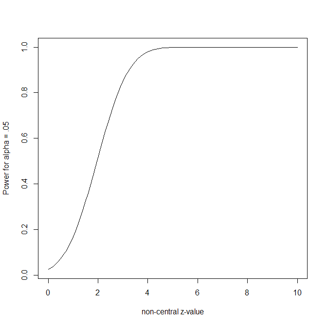
Hoenig and Heisey’s main point was that sampling error and conditioning on statistical significance lead to misleading claims about power. If a study produced a significant result, post-hoc power cannot be very low, because the observed effect-size estimate had to be large enough relative to its standard error to cross the significance threshold. For z-values, a two-sided p-value of .05 corresponds to a critical value of about 1.96. Thus, a significant result requires an estimate that is about two standard errors away from zero. The reverse is true for nonsignificant results. Studies that fail to reach significance will tend to produce low post-hoc power estimates. Researchers who obtain significant results therefore get observed-power estimates that look moderate or high, whereas researchers who obtain nonsignificant results get observed-power estimates that look low. The fallacy is to assume that these values represent the true power of the study. Significant results were not necessarily obtained with moderate or high power, and nonsignificant results cannot automatically be attributed to low power.
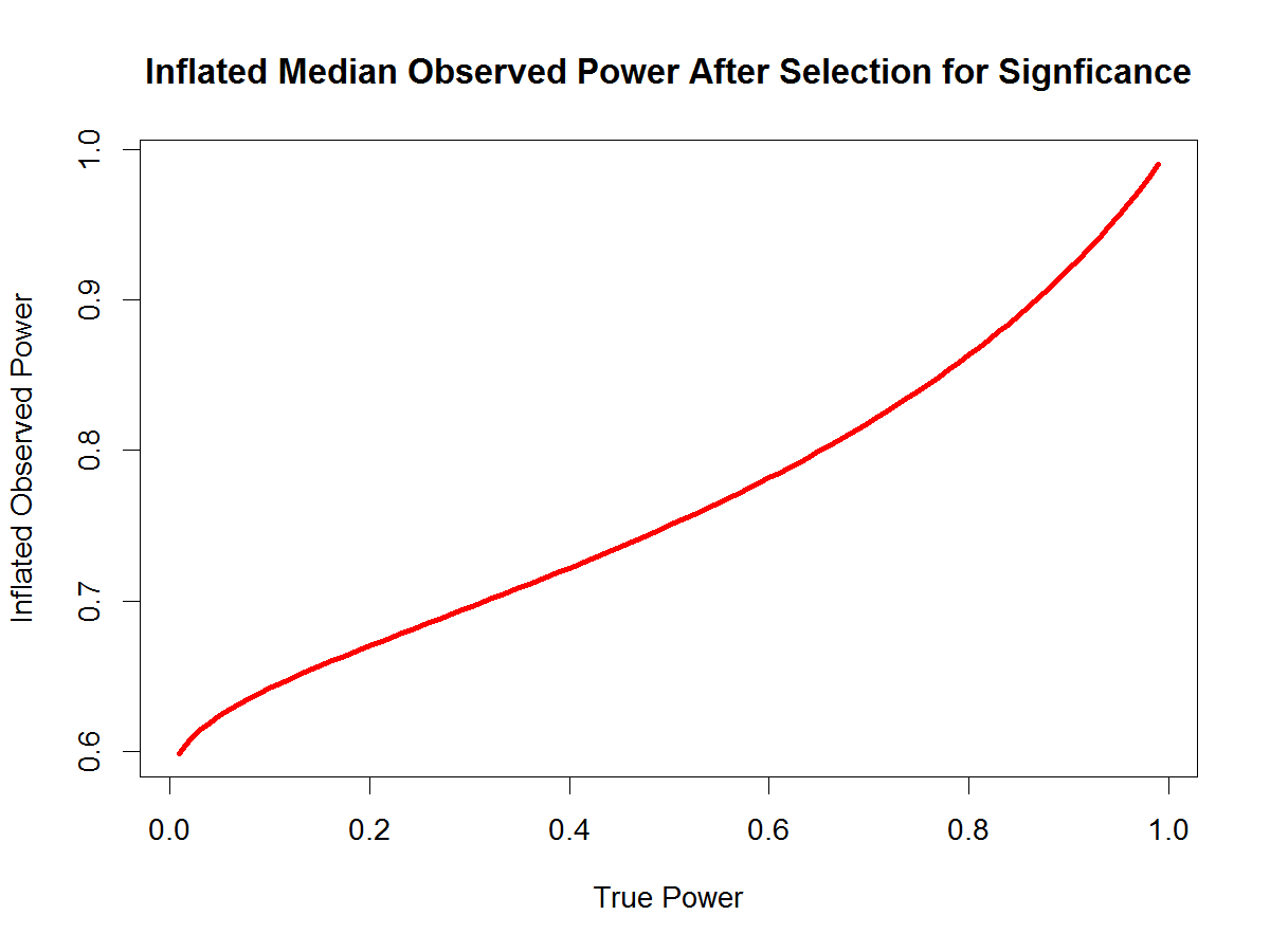
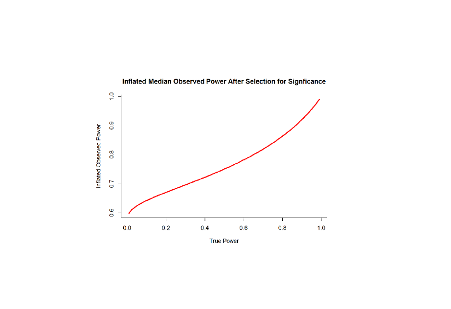
Selection for significance means that the estimates are biased. When results are selected because they are statistically significant, the observed effects are typically larger than the true effects. This is a form of regression to the mean, although the mean itself is unknown. If all significant results were false positives, the true probability of obtaining a significant result would simply be the Type I error rate, typically 5%. Yet the observed power of significant false positives is much higher (~ 62% on average) This shows how dangerous it is to confuse post-hoc power with true power.
The Omitted Warning About Post-Hoc Effect-Size Calculations
The previous discussion shows that the problem with post-hoc power calculations is not the calculations. The problem is that the calculation treats the observed effect-size estimate as if it were the true population effect. When a result is selected because it is statistically significant, this assumption is often misleading. Significant results from small studies tend to have inflated effect-size estimates because only estimates large enough to cross the significance threshold are likely to be noticed, reported, or published. Thus, the root problem is biased effect-size estimation, not the conversion of an effect-size estimate into a power estimate.
This creates an odd asymmetry in current statistical practice. Reporting effect-size estimates from observed data is widely recommended and often required, whereas using the same estimates to compute post-hoc power is widely dismissed as a fallacy. But if post-hoc power is misleading because it is based on a noisy and selected effect-size estimate, then the same concern applies to the selected effect-size estimate itself.
The importance of this concern varies across research areas. In some fields, effect-size estimation is the central goal. Public opinion polling is a simple example. A poll with a reasonably large sample may estimate support for a candidate with a margin of error of only a few percentage points. In that setting, the point estimate is useful because the estimate is relatively precise and is not usually selected for publication because it crossed an arbitrary significance threshold.
The situation is different in many areas of psychology. Sample sizes are often small, standard errors are large, and the incentive structure rewards statistically significant findings. Since the 1950s, reviews of the psychological literature have shown that the large majority of published articles report at least one statistically significant result used to support a substantive claim (Sterling, 1959; Sterling et al., 1995). In this context, post-hoc effect sizes calculations can be highly misleading. A study may provide evidence about the direction of an effect, but the reported effect size can be much larger than the true population effect.
I am not the first to note that selection for statistical significance inflates effect-size estimates from small studies. Button et al. (2013), for example, emphasized that low-powered studies produce exaggerated estimates and unreliable findings. However, this literature has generally stopped short of treating routine interpretation of selected effect-size estimates with the same severity as post-hoc power analysis. This is striking because both quantities are compromised by the same input: a noisy effect-size estimate selected because it crossed a significance threshold.
The problem is especially serious when the observed effect size looks impressive precisely because the study had low precision. In a small study, statistical significance often requires a large observed effect. As a result, the studies least able to estimate the true effect accurately are also the studies most likely to report exaggerated effect sizes when they are significant. The ego-depletion literature illustrates this problem. Early post-hoc effect sizes suggested a sizable average effect, whereas later large-scale tests with small confidence intervals produced small post-hoc estimates and the confidence interval still included zero, suggesting that many studies reported notable post-hoc effect sizes when the true value was practically zero..
Thus, reporting observed effect-size estimates from significance-selected studies can have the same basic problem as reporting post-hoc power. The values may look informative, but they can be driven by the same selected and inflated estimate. The result is a misleading evidential package: a significant p-value, a seemingly large effect size, and sometimes a high observed-power estimate, all derived from the same noisy result.
Hoenig and Heisey’s warning about post-hoc calculations therefore applies not only to post-hoc power calculations, but also to post-hoc effect size calculations. The issue is not that one calculation is inherently fallacious while the other is automatically good practice. The issue is that both can be misleading when researchers treat selected, imprecise estimates as if they revealed the true magnitude of an effect.
Confidence Intervals as Conservative Hypothesis Tests
The previous discussion shows that the problem is inherent in the data, not in a particular calculation based on the data. Studies with large standard errors provide imprecise quantitative information. The central task of statistical inference is to represent this uncertainty honestly.
The solution is nearly a century old and is associated with Neyman’s theory of confidence intervals. Given an acceptable error rate, such as 5%, uncertainty in an estimate can be represented by adding and subtracting approximately two standard errors from the observed estimate. In the long run, under the assumptions of the model, this interval will contain the true value 95% of the time. The remaining 5% of intervals will miss the true value because sampling error moved the estimate too far upward or downward.
Confidence intervals are familiar to most people because they are used in public opinion polling. Assuming unbiased sampling of respondents, election polls will contain the true population value within the reported margin of error approximately 95% of the time. The same logic applies in fields with larger sampling error, but the resulting intervals can be very wide. Cohen (1994) speculated that psychologists were reluctant to report confidence intervals because they could be embarrassingly wide. A study might report an impressive value of a post-hoc effect size calculation, d = .60, but the 95% confidence interval might range from d = .06 to d = 1.14. This interval covers nearly the full range of plausible effect sizes without any data collection. In such a case, the point estimate of d = .60, is misleading and fails to alert readers that the true effect size could be close to zero.
Psychology has gradually embraced the reporting of confidence intervals as a good practice, but confidence intervals are often treated as secondary qualifications attached to the value from a post-hoc effect size calculation. The fallacy is to focus on this single value and to ignore the wide range of equally plausible values. In practice, many articles focus on the single post-hoc value and ignore the wide range of other values that are compatible with the data.
The proper use of confidence intervals is to treat them as conservative hypothesis tests. A confidence interval that does not include zero can support a directional claim. If the lower bound of the interval is d = .06, the study provides evidence that the true effect is positive. However, it does not justify the claim that the effect is moderate or large simply because the post-hoc effect size value is moderate or large. The study rules out values below the lower limit of the interval. It does not rule out small positive effects. The appropriate conclusion is therefore limited: the effect is likely positive and larger than d = .06. That is the only magnitude claim the study can support.
Confidence intervals do not solve the problem of selection bias. When studies are selected because they are statistically significant, the entire interval can be shifted upward, including the lower bound. Thus, even a lower bound such as d = .06 may still be inflated; the true effect could be smaller, zero, or even negative. Nevertheless, confidence intervals reduce the abuse of post-hoc calculations because they prevent researchers from making strong claims about the size of an effect when the data do not warrant such claims. A study with an observed effect of d = .60 and a confidence interval from d = .06 to d = 1.14 may justify the limited claim that the result is statistically compatible with a positive effect, but it does not justify the stronger claim that the study demonstrated a moderate or large effect.
The same logic applies to nonsignificant results in psychology. A nonsignificant result is not automatically uninformative. It is uninformative when the confidence interval is so wide that it fails to rule out effects that would matter theoretically or practically. Conversely, a nonsignificant result can be highly informative when the confidence interval is narrow enough to rule out effects of meaningful size. This point deserves its own discussion, but for the present argument the lesson is simple: the evidential value of a result depends less on whether p is below .05 than on what values the confidence interval rules out..
To encourage the proper use of confidence intervals, we should reconsider the prominent reporting of post-hoc effect-size values in low-precision studies. For example, we could require that sampling error is less than .1 or some criterion of sufficient precision before articles report point estimates.
Of course, point estimates are needed to compute confidence intervals and reporting them is not the real problem. The problem is when they are treated as the headline result when the interval is wide. In such cases, the post-hoc effect size values are just as misleading as post-hoc power values. Moreover, the focus on post-hoc effect size values rewards researchers who selectively publish large effects from small samples and report impressive and inflated values, while disadvantaging researchers who invest resources in studies with narrow confidence intervals that provide actual quantitative information about true effect sizes.
Calling post-hoc effect size calculations a fallacy may seem radical, but it is consistent with Hoenig and Heisey’s widely accepted warning against post-hoc power calculations. “Observed power” is misleading because it is easily mistaken for true power. “Observed effect-sizes” are misleading for the same reason: they are easily mistaken for true effect sizes. The key fallacy is not a particular statistical calculation. The key fallacy is confusing uncertain estimates with the true values they are meant to estimate.
In short, it is time to treat post-hoc effect sizes with the same suspicion as post-hoc power values. This does not mean that we should avoid quantifying effects size estimates. We just need to remember that all estimates are estimates are estimates and not confuse estimates with unknown true values. Neyman provided us with a statistical tool to do so. We just have to start using it properly in psychology as it is already being used in other fields.