Category Archives: Research Integrity

Replicability 101: How to interpret the results of replication studies

Even statistically sophisticated psychologists struggle with the interpretation of replication studies (Maxwell et al., 2015).  This article gives a basic introduction to the interpretation of statistical results within the Neyman Pearson approach to statistical inferences.

I make two important points and correct some potential misunderstandings in Maxwell et al.’s discussion of replication failures.  First, there is a difference between providing sufficient evidence for the null-hypothesis (evidence of absence) and providing insufficient evidence against the null-hypothesis (absence of evidence).  Replication studies are useful even if they simply produce absence of evidence without evidence that an effect is absent.  Second, I  point out that publication bias undermines the credibility of significant results in original studies.  When publication bias is present, open replication studies are valuable because they provide an unbiased test of the null-hypothesis, while original studies are rigged to reject the null-hypothesis.

DEFINITION OF REPLICATING A STATISTICAL RESULT

Replicating something means to get the same result.  If I make the first free throw, replicating this outcome means to also make the second free throw.  When we talk about replication studies in psychology we borrow from the common meaning of the term “to replicate.”

If we conduct psychological studies, we can control many factors, but some factors are not under our control.  Participants in two independent studies differ from each other and the variation in the dependent variable across samples introduces sampling error. Hence, it is practically impossible to get identical results, even if the two studies are exact copies of each other.  It is therefore more complicated to compare the results of two studies than to compare the outcome of two free throws.

To determine whether the results of two studies are identical or not, we need to focus on the outcome of a study.  The most common outcome in psychological studies is a significant or non-significant result.  The goal of a study is to produce a significant result and for this reason a significant result is often called a success.  A successful replication study is a study that also produces a significant result.  Obtaining two significant results is akin to making two free throws.  This is one of the few agreements between Maxwell and me.

“Generally speaking, a published  original study has in all likelihood demonstrated a statistically significant effect. In the current zeitgeist, a replication study is usually interpreted as successful if it also demonstrates a statistically significant effect.” (p. 488)

The more interesting and controversial scenario is a replication failure. That is, the original study produced a significant result (success) and the replication study produced a non-significant result (failure).

I propose that a lot of confusion arises from the distinction between original and replication studies. If a replication study is an exact copy of the first study, the outcome probabilities of original and replication studies are identical.  Otherwise, the replication study is not really a replication study.

There are only three possible outcomes in a set of two studies: (a) both studies are successful, (b) one study is a success and one is a failure, or (c) both studies are failures.  The probability of these outcomes depends on whether the significance criterion (the type-I error probability) when the null-hypothesis is true and the statistical power of a study when the null-hypothesis is false.

Table 1 shows the probability of the outcomes in two studies.  The uncontroversial scenario of two significant results is very unlikely, if the null-hypothesis is true. With conventional alpha = .05, the probability is .0025 or 1 out of 400 attempts.  This shows the value of replication studies. False positives are unlikely to repeat themselves and a series of replication studies with significant results is unlikely to occur by chance alone.

2 sig, 0 ns 1 sig, 1 ns 0 sig, 2 ns
H0 is True alpha^2 2*alpha*(1-alpha) (1-alpha^2)
H1 is True (1-beta)^2 2*(1-beta)*beta beta^2

The probability of a successful replication of a true effect is a function of statistical power (1 – type-II error probability).  High power is needed to get significant results in a pair of studies (an original study and a replication study).  For example, if power is only 50%, the chance of this outcome is only 25% (Schimmack, 2012).  Even with conventionally acceptable power of 80%, only 2/3 (64%) of replication attempts would produce this outcome.  However, studies in psychology do not have 80% power and estimates of power can be as low as 37% (OSC, 2015). With 40% power, a pair of studies would produce significant results in no more than 16 out of 100 attempts.   Although successful replications of true effects with low power are unlikely, they are still much more likely then significant results when the null-hypothesis is true (16/100 vs. 1/400 = 64:1).  It is therefore reasonable to infer from two significant results that the null-hypothesis is false.

If the null-hypothesis is true, it is extremely likely that both studies produce a non-significant result (.95^2 = 90.25%).  In contrast, it is unlikely that even a study with modest power would produce two non-significant results.  For example, if power is 50%, there is a 75% chance that at least one of the two studies produces a significant result. If power is 80%, the probability of obtaining two non-significant results is only 4%.  This means, it is much more likely (22.5 : 1) that the null-hypothesis is true than that the alternative hypothesis is true.  This does not mean that the null-hypothesis is true in an absolute sense because power depends on the effect size.  For example, if 80% power were obtained with a standardized effect size of Cohen’s d = .5,  two non-significant results would suggest that the effect size is smaller than .5, but it does not warrant the conclusion that H0 is true and the effect size is exactly 0.  Once more, it is important to distinguish between the absence of evidence for an effect and the evidence of absence of an effect.

The most controversial scenario assumes that the two studies produced inconsistent outcomes.  Although theoretically there is no difference between the first and the second study, it is common to focus on a successful outcome followed by a replication failure  (Maxwell et al., 2015). When the null-hypothesis is true, the probability of this outcome is low;  .05 * (1-.05) = .0425.  The same probability exists for the reverse pattern that a non-significant result is followed by a significant one.  A probability of 4.25% shows that it is unlikely to observe a significant result followed by a non-significant result when the null-hypothesis is true. However, the low probability is mostly due to the low probability of obtaining a significant result in the first study, while the replication failure is extremely likely.

Although inconsistent results are unlikely when the null-hypothesis is true, they can also be unlikely when the null-hypothesis is false.  The probability of this outcome depends on statistical power.  A pair of studies with very high power (95%) is very unlikely to produce an inconsistent outcome because both studies are expected to produce a significant result.  The probability of this rare event can be as low, or lower, than the probability with a true null effect; .95 * (1-.95) = .0425.  Thus, an inconsistent result provides little information about the probability of a type-I or type-II  error and is difficult to interpret.

In conclusion, a pair of significance tests can produce three outcomes. All three outcomes can occur when the null-hypothesis is true and when it is false.  Inconsistent outcomes are likely unless the null-hypothesis is true or the null-hypothesis is false and power is very high.  When two studies produce inconsistent results, statistical significance provides no basis for statistical inferences.

Meta-Analysis 

The counting of successes and failures is an old way to integrate information from multiple studies.  This approach has low power and is no longer used.  A more powerful approach is effect size meta-analysis.  Effect size meta-analysis was one way to interpret replication results in the Open Science Collaboration (2015) reproducibility project.  Surprisingly, Maxwell et al. (2015) do not consider this approach to the interpretation of failed replication studies. To be clear, Maxwell et al. (2015) mention meta-analysis, but they are talking about meta-analyzing a larger set of replication studies, rather than meta-analyzing the results of an original and a replication study.

“This raises a question about how to analyze the data obtained from multiple studies. The natural answer is to use meta-analysis.” (p. 495)

I am going to show that effect-size meta-analysis solves the problem of interpreting inconsistent results in pairs of studies. Importantly, effect size meta-analysis does not care about significance in individual studies.  A meta-analysis of a pair of studies with inconsistent results is no different from a meta-analysis of a pair of studies with consistent results.

Maxwell et al.’s (2015) introduced an example of a between-subject (BS) design with n = 40 per group (total N = 80) and a standardized effect size of Cohen’s d = .5 (a medium effect size).  This study has 59% power to obtain a significant result.  Thus, it is quite likely that a pair of studies produces inconsistent results (48.38%).   However, a pair of studies with N = 80 has the power of a total sample size of N = 160, which means a fixed-effects meta-analysis will produce a significant result in 88% of all attempts.  Thus, it is not difficult at all to interpret the results of pairs of studies with inconsistent results if the studies have acceptable power (> 50%).   Even if the results are inconsistent, a meta-analysis will provide the correct answer that there is an effect most of the time.

A more interesting scenario are inconsistent results when the null-hypothesis is true.  I turned to simulations to examine this scenario more closely.   The simulation showed that a meta-analysis of inconsistent studies produced a significant result in 34% of all cases.  The percentage slightly varies as a function of sample size.  With a small sample of N = 40, the percentage is 35%. With a large sample of  1,000 participants it is 33%.  This finding shows that in two-thirds of attempts, a failed replication reverses the inference about the null-hypothesis based on a significant original study.  Thus, if an original study produced a false-positive results, a failed replication study corrects this error in 2 out of 3 cases.  Importantly, this finding does not warrant the conclusion that the null-hypothesis is true. It merely reverses the result of the original study that falsely rejected the null-hypothesis.

In conclusion, meta-analysis of effect sizes is a powerful tool to interpret the results of replication studies, especially failed replication studies.  If the null-hypothesis is true, failed replication studies can reduce false positives by 66%.

DIFFERENCES IN SAMPLE SIZES

We can all agree that, everything else being equal, larger samples are better than smaller samples (Cohen, 1990).  This rule applies equally to original and replication studies. Sometimes it is recommended that replication studies should use much larger samples than original studies, but it is not clear to me why researchers who conduct replication studies should have to invest more resources than original researchers.  If original researchers conducted studies with adequate power,  an exact replication study with the same sample size would also have adequate power.  If the original study was a type-I error, the replication study is unlikely to replicate the result no matter what the sample size.  As demonstrated above, even a replication study with the same sample size as the original study can be effective in reversing false rejections of the null-hypothesis.

From a meta-analytic perspective, it does not matter whether a replication study had a larger or smaller sample size.  Studies with larger sample sizes are given more weight than studies with smaller samples.  Thus, researchers who invest more resources are rewarded by giving their studies more weight.  Large original studies require large replication studies to reverse false inferences, whereas small original studies require only small replication studies to do the same.  Nevertheless, failed replications with larger samples are more likely to reverse false rejections of the null-hypothesis, but there is no magical number about the size of a replication study to be useful.

I simulated a scenario with a sample size of N = 80 in the original study and a sample size of N = 200 in the replication study (a factor of 2.5).  In this simulation, only 21% of meta-analyses produced a significant result.  This is 13 percentage points lower than in the simulation with equal sample sizes (34%).  If the sample size of the replication study is 10 times larger (N = 80 and N = 800), the percentage of remaining false positive results in the meta-analysis shrinks to 10%.

The main conclusion is that even replication studies with the same sample size as the original study have value and can help to reverse false positive findings.  Larger sample sizes simply give replication studies more weight than original studies, but it is by no means necessary to increase sample sizes of replication studies to make replication failures meaningful.  Given unlimited resources, larger replications are better, but these analysis show that large replication studies are not necessary.  A replication study with the same sample size as the original study is more valuable than no replication study at all.

CONFUSING ABSENCE OF EVIDENCE WITH EVIDENCE OF ABSENCE

One problem in Maxwell et al’s (2015) article is to conflate two possible goals of replication studies.  One goal is to probe the robustness of the evidence against the null-hypothesis. If the original result was a false positive result, an unsuccessful replication study can reverse the initial inference and produce a non-significant result in a meta-analysis.  This finding would mean that evidence for an effect is absent.  The status of a hypothesis (e.g., humans have supernatural abilities; Bem, 2011) is back to where it was before the original study found a significant result and the burden of proof is shifted back to proponents of the hypothesis to provide unbiased credible evidence for it.

Another goal of replication studies can be to provide conclusive evidence that an original study reported a false positive result (i..e, humans do not have supernatural abilities).  Throughout their article, Maxwell et al. assume that the goal of replication studies is to prove the absence of an effect.  They make many correct observations about the difficulties of achieving this goal, but it is not clear why replication studies have to be conclusive when original studies are not held to the same standard.

This makes it easy to produce (potentially false) positive results and very hard to remove false positive results from the literature.   It also creates a perverse incentive to conduct underpowered original studies and to claim victory when a large replication study finds a significant result with an effect size that is 90% smaller than the effect size in an original study.  The authors of the original article may claim that they do not care about effect sizes and that their theoretical claim was supported.  To avoid this problem that replication researchers have to invest large amount of resources for little gain, it is important to realize that even a failure to replicate an original finding with the same sample size can undermine original claims and force researchers to provide stronger evidence for their original ideas in original articles.  If they are right and the evidence is strong, others will be able to replicate the result in an exact replication study with the same sample size.

THE DIRTY BIG SECRET

The main problem of Maxwell et al.’s (2015) article is that the authors blissfully ignore the problem of publication bias.  They mention publication bias twice to warn readers that publication bias inflates effect sizes and biases power analyses, but they completely ignore the influence of publication bias on the credibility of successful original results (Schimmack, 2012; Sterling; 1959; Sterling et al., 1995).

It is hard to believe that Maxwell is unaware of this problem, if only because Maxwell was action editor of my article that demonstrated how publication bias undermines the credibility of replication studies that are selected for significance  (Schimmack, 2012).

I used Bem’s infamous article on supernatural abilities as an example, which appeared to show 8 successful replications of supernatural abilities.  Ironically, Maxwell et al. (2015) also cites Bem’s article to argue that failed replication studies can be misinterpreted as evidence of absence of an effect.

“Similarly, Ritchie, Wiseman, and French (2012) state that their failure to obtain significant results in attempting to replicate Bem (2011) “leads us to favor the ‘experimental artifacts’ explanation for Bem’s original result” (p. 4)”

This quote is not only an insult to Ritchie et al.; it also ignores the concerns that have been raised about Bem’s research practices. First, Ritchie et al. do not claim that they have provided conclusive evidence against ESP.  They merely express their own opinion that they “favor the ‘experimental artifacts’ explanation.  There is nothing wrong with this statement, even if it is grounded in a healthy skepticism about supernatural abilities.

More important, Maxwell et al. ignore the broader context of these studies.  Schimmack (2012) discussed many questionable practices in Bem’s original studies and I presented statistical evidence that the significant results in Bem’s article were obtained with the help of questionable research practices.  Given this wider context, it is entirely reasonable to favor the experimental artifact explanation over the alternative hypothesis that learning after an exam can still alter the exam outcome.

It is not clear why Maxwell et al. (2015) picked Bem’s article to discuss problems with failed replication studies and ignores that questionable research practices undermine the credibility of significant results in original research articles. One reason why failed replication studies are so credible is that insiders know how incredible some original findings are.

Maxwell et al. (2015) were not aware that in the same year, the OSC (2015) reproducibilty project would replicate only 37% of statistically significant results in top psychology journals, while the apparent success rate in these journals is over 90%.  The stark contrast between the apparent success rate and the true power to produce successful outcomes in original studies provided strong evidence that psychology is suffering from a replication crisis. This does not mean that all failed replications are false positives, but it does mean that it is not clear which findings are false positives and which findings are not.  Whether this makes things better is a matter of opinion.

Publication bias also undermines the usefulness of meta-analysis for hypothesis testing.  In the OSC reproducibility project, a meta-analysis of original and replication studies produced 68% significant results.  This result is meaningless because publication bias inflates effect sizes and the probability of obtaining a false positive result in the meta-analysis. Thus, when publication bias is present, unbiased replication studies provide the most credible evidence and the large number of replication failures means that more replication studies with larger samples are needed to see which hypothesis predict real effects with practical significance.

DOES PSYCHOLOGY HAVE A REPLICATION CRISIS?

Maxwell et al.’s (2015) answer to this question is captured in this sentence. “Despite raising doubts about the extent to which apparent failures to replicate necessarily reveal that psychology is in crisis,we do not intend to dismiss concerns about documented methodological flaws in the field.” (p. 496).  The most important part of this quote is “raising doubt,” the rest is Orwellian double-talk.

The whole point of Maxwell et al.’s article is to assure fellow psychologists that psychology is not in crisis and that failed replication studies should not be a major concern.  As I have pointed out, this conclusion is based on some misconceptions about the purpose of replication studies and by blissful ignorance about publication bias and questionable research practices that made it possible to publish successful replications of supernatural phenomena, while discrediting authors who spend time and resources on demonstrating that unbiased replication studies fail.

The real answer to Maxwell et al.’s question was provided by the OSC (2015) finding that only 37% of published significant results could be replicated.  In my opinion that is not only a crisis, but a scandal because psychologists routinely apply for funding with power analyses that claim 80% power.  The reproducibilty project shows that the true power to obtain significant results in original and replication studies is much lower than this and that the 90% success rate is no more meaningful than 90% votes for a candidate in communist elections.

In the end, Maxwell et al. draw the misleading conclusion that “the proper design and interpretation of replication studies is less straightforward than conventional practice would suggest.”  They suggest that “most importantly, the mere fact that a replication study yields a nonsignificant statistical result should not by itself lead to a conclusion that the corresponding original study was somehow deficient and should no longer be trusted.”

As I have demonstrated, this is exactly the conclusion that readers should draw from failed replication studies, especially if (a) the original study was not preregistered, (b) the original study produced weak evidence (e.g., p = .04), the original study was published in a journal that only publishes significant results, (d) the replication study had a larger sample, (e) the replication study would have been published independent of outcome, and (f) the replication study was preregistered.

We can only speculate why the American Psychologists published a flawed and misleading article that gives original studies the benefit of the doubt and casts doubt on the value of replication studies when they fail.  Fortunately, APA can no longer control what is published because scientists can avoid the censorship of peer-reviewed journals by publishing blogs and by criticize peer-reviewed articles in open post-publication peer review on social media.

Long life the replicability revolution.  !!!

REFERENCES

Cohen, J. (1990). Things I have learned (so far). American Psychologist, 45(12), 1304-1312.

http://dx.doi.org/10.1037/0003-066X.45.12.1304

Maxwell, S.E, Lau, M. Y., & Howard, G. S. (2015). Is psychology suffering from a replication crisis? What does ‘failure to replicate’ really mean? American Psychologist, 70, 487-498. http://dx.doi.org/10.1037/a0039400.

Schimmack, U. (2012). The ironic effect of significant results on the credibility of multiple-study articles. Psychological Methods, 17(4), 551-566. http://dx.doi.org/10.1037/a0029487


Hidden Figures: Replication Failures in the Stereotype Threat Literature

In the past five years, it has become apparent that many classic and important findings in social psychology fail to replicate (Schimmack, 2016).  The replication crisis is often considered a new phenomenon, but failed replications are not entirely new.  Sometimes these studies have simply been ignored.  These studies deserve more attention and need to be reevaluated in the context of the replication crisis in social psychology.

In the past, failed replications were often dismissed because seminal articles were assumed to provide robust empirical support for a phenomenon, especially if an article presented multiple studies. The chance of reporting a false positive results in a multiple study article is low because the risk of a false positive decreases exponentially (Schimmack, 2012). However, the low risk of a false positive is illusory if authors only publish studies that worked. In this case, even false positives can be supported by significant results in multiple studies, as demonstrated in the infamous ESP study by Bem (2011).  As a result, publication bias undermines the reporting of statistical significance as diagnostic information about the risk of false positives (Sterling, 1959) and many important theories in social psychology rest on shaky empirical foundations that need to be reexamined.

Research on stereotype threat and women’s performance on math tests is one example where publication bias undermines the findings in a seminal study that produced a large literature of studies on gender differences in math performance. After correcting for publication bias, this literature shows very little evidence that stereotype threat has a notable and practically significant effect on women’s math performance (Flore & Wicherts, 2014).

Another important line of research has examined the contribution of stereotype threat to differences between racial groups on academic performance tests.  This blog post examines the strength of the empirical evidence for stereotype threat effects in the seminal article by Steele and Aronson (1995). This article is currently the 12th most cited article in the top journal for social psychology, Journal of Personality and Social Psychology (2,278 citations so far).

According to the abstract, “stereotype threat is being at risk of confirming, as self-characteristic, a negative stereotype about one’s group.” Studies 1 and 2 showed that “reflecting the pressure of this vulnerability, Blacks underperformed in relation to Whites in the ability-diagnostic condition but not in the nondiagnostic condition (with Scholastic Aptitude Tests controlled).”  “Study 3 validated that ability-diagnosticity cognitively activated the racial stereotype in these participants and motivated them not to conform to it, or to be judged by it.”  “Study 4 showed that mere salience of the stereotype could impair Blacks’ performance even when the test was not
ability diagnostic.”

The results of Study 4 motivated Stricker and colleagues to examine the influence of stereotype-treat on test performance in a real-world testing situation.  These studies had large samples and were not limited to students at Stanford. One study was reported in a College Board Report (Stricker and Ward, 1998).   Another two studies were published in the Journal of Applied Social Psychology (Stricker & Ward, 2004).  This article received only 52 citations, although it reported two studies with an experimental manipulation of stereotype threat in a real assessment context.  One group of participants were asked about their gender or ethnicity before the text, the other group did not receive these questions.  As noted in the abstract, neither the inquiry about race, nor about gender, had a significant effect on test performance. In short, this study failed to replicate Study 4 of the classic and widely cited article by Steele and Aronson.

Stricker and Ward’s Abstract
Steele and Aronson (1995) found that the performance of Black research participants on
ability test items portrayed as a problem-solving task, in laboratory experiments, was affected adversely when they were asked about their ethnicity. This outcome was attributed to stereotype threat: Performance was disrupted by participants’ concerns about fulfilling the negative stereotype concerning Black people’s intellectual ability. The present field experiments extended that research to other ethnic groups and to males and females taking operational tests. The experiments evaluated the effects of inquiring about ethnicity and gender on the performance of students taking 2 standardized tests-the Advanced Placement Calculus AB Examination, and the Computerized Placement Tests-in actual test administrations. This inquiry did not have any effects on the test performance of Black, female, or other subgroups of students that were both statistically and practically significant.

The article also mentions a personal communication with Steele, in which Steele mentions an unpublished study that also failed to demonstrate the effect under similar conditions.

“In fact, Steele found in an unpublished pilot study that inquiring about ethnicity did not affect Black participants’ performance when the task was described as diagnostic of their ability (C. M. Steele, personal communication, May 2 1, 1997), in contrast to the
substantial effect of inquiring when the task was described as nondiagnostic.”

A substantive interpretation of this finding is that inquires about race or gender do not produce stereotype threat effects when a test is diagnostic because a diagnostic test already activates stereotype threat.  However, if this were a real moderator, it would be important to document this fact and it is not clear why this finding obtained in an earlier study by Steele remained unpublished. Moreover, it is premature to interpret the significant result in the published study with a non-diagnostic task and the non-significant result in an unpublished study with a diagnostic task as evidence that diagnosticity moderates the effect of the stereotype-threat manipulation. A proper test of this moderator hypothesis would require the demonstration of a three-way interaction between race, inquiry about race, and diagnosticity. Absent this evidence, it remains possible that diagnosticity is not a moderator and that the published result is a false positive (or a positive result with an inflated effect size estimate). In contrast, there appears to be consistent evidence that inquiries about race or gender before a real assessment of academic performance does not influence performance. This finding is not widely publicized, but is important for a better understanding of performance differences in real world settings.

The best way to examine the replicability of Steele and Aronson’s seminal finding with non-diagnostic tasks would be to conduct an exact replication study.  However, exact replication studies are difficult and costly.  An alternative is to examine the robustness of the published results by taking a closer look at the strength of the statistical results reported by Steele and Aronson, using modern statistical tests of publication bias and statistical power like the R-Index (Schimmack, 2014) and the Test of Insufficient Variance (TIVA, Schimmack, 2014).

Replicability Analysis of Steele and Aronson’s four studies

Study 1. The first study had a relatively large sample of N = 114 participants, but it is not clear how many of the participants were White or Black.  The study also had a 2 x 3 design, which leaves less than 20 participants per condition.   The study produced a significant main effect of condition, F(2, 107) = 4.74, and race, F(1,107) = 5.22, but the critical condition x race interaction was not significant (reported as p > .19).   However, a specific contrast showed significant differences between Black participants in the diagnostic condition and the non-diagnostic condition, t(107) = 2.88, p = .005, z = 2.82.  The authors concluded “in sum, then, the hypothesis was supported by the pattern of contrasts, but when tested over the whole design, reached only marginal significance” (p. 800).  In other words, Study 1 provided only weak support for the stereotype threat hypothesis.

Study 2. Study 2 eliminated one of the three experimental conditions. Participants were 20 Black and 20 White participants. This means there were only 10 participants in each condition of a 2 x 2 design. The degrees of freedom further indicate that the actual sample size was only 38 participants. Given the weak evidence in Study 1, there is no justification for a reduction in the number of participants per cell, although the difficulty of recruiting Black participants at Stanford may explain this inadequate sample size. Nevertheless, the study showed a significant interaction between race and test description, F(1,35) = 8.07, p = .007. The study also replicated the contrast from Study 1 that Black participants in the diagnostic condition performed significantly worse than Black participants in the non-diagnostic group, t(35) = 2.38, p = .023, z = 2.28.

Studies 1 and 2 are close replications of each other.  The consistent finding across the two studies that supports stereotype-treat theory is the finding that merely changing the description of an assessment task changes Black participants performance, as revealed by significant differences between the diagnostic and non-diagnostic condition in both studies.  The problem is that both studies had small numbers of Black participants and that small samples have low power to produce significant results. As a result, it is unlikely that a pair of studies would produce significant results in both studies.

Observed power  in the two studies is .81 and .62 with median observed power of .71. Thus, the actual success rate of 100% (2 out of 2 significant results) is 29 percentage points higher than the expected success rate. Moreover, when inflation is evident, median observed power is also inflated. To correct for this inflation, the Replicability-Index (R-Index) subtracts inflation from median observed power, which yields an R-Index of 42.  Any value below 50 is considered unacceptably low and I give it a letter grade F, just like students at American Universities receive an F for exams with less than 50% correct answers.  This does not mean that stereotype threat is not a valid theory or that there was no real effect in this pair of studies. It simply means that the evidence in this highly cited article is insufficient to make strong claims about the causes of Black’s performance on academic tests.

The Test of Insufficient Variance (TIVA) provides another way to examine published results.  Test statistics like t-values vary considerably from study to study even if the exact same study is conducted twice (or if one larger sample is randomly split into two sub-samples).  When test-statistics are converted into z-scores, sampling error (the random variability from sample to sample) follows approximately a standard normal distribution with a variance of 1.  If the variance is considerably smaller than 1, it suggests that the reported results represent a selected sample. Often the selection is a result of publication bias.  Applying TIVA to the pair of studies, yields a variance of Var(z) = 0.15.  As there are only two studies, it is possible that this outcome occurred by chance, p = .300, and it does not imply intentional selection for significance or other questionable research practices.  Nevertheless, it suggests that future replication studies will be more variable and produce some non-significant results.

In conclusion, the evidence presented in the first two studies is weaker than we might assume if we focused only on the fact that both studies produced significant contrasts. Given publication bias, the fact that both studies reported significant results provides no empirical evidence because virtually all published studies report significant results. The R-Index quantifies the strength of evidence for an effect while taking the influence of publication bias into account and it shows that the two studies with small samples provide only weak evidence for an effect.

Study 3.  This study did not examine performance. The aim was to demonstrate activation of stereotype threat with a sentence completion task.  The sample size of 68 participants  (35 Black, 33 White) implied that only 11 or 12 participants were assigned to one of the six cells in a 2 (race) by 3 (task description) design. The study produced main effects for race and condition, but most importantly it produced a significant interaction effect, F(2,61) = 3.30, p = .044.  In addition, Black participants in the diagnostic condition had more stereotype-related associations than Black participants in the non-diagnostic condition, t(61) = 3.53,

Study 4.  This study used inquiry about race to induce stereotype-threat. Importantly, the task was described as non-diagnostic (as noted earlier, a similar study produced no significant results when the task was described as diagnostic).  The design was a 2 x 2 design with 47 participants, which means only 11 or 12 participants were allocated to the four conditions.  The degrees of freedom indicated that cell frequencies were even lower. The study produced a significant interaction effect, F(1,39) = 7.82, p = .008.  The study also produced a significant contrast between Blacks in the race-prime condition and the no-prime condition, t(39) = 2.43, p = .020.

The contrast effect in Study 3 is strong, but it is not a performance measure.  If stereotype threat mediates the effect of task characteristics and performance, we would expect a stronger effect on the measure of the mediator than on the actual outcome of interest, task performance.  The key aim of stereotype threat theory is to explain differences in performance.  With a focus on performance outcomes, it is possible to examine the R-Index and TIVA of Studies 1, 2, and 4.  All three studies reported significant contrasts between Black students randomly assigned to two groups that were expected to show performance differences (Table 1).

Table 1

Study Test Statistic p-value z-score obs.pow
Study 1 t(107) = 2.88 0.005 2.82 0.81
Study 2 t(35)=2.38 0.023 2.28 0.62
Study 4 t(39) = 2.43 0.020 2.33 0.64

Median observed power is 64 and the R-Index is well below 50, 64 – 36 = 28 (F).  The variance in z-scores is Var(z) = 0.09, p = .086.  These results cast doubt about the replicability of the performance effects reported in Steele and Aronson’s seminal stereotype threat article.

Conclusion

Racial stereotypes and racial disparities are an important social issue.  Social psychology aims and promises to contribute to the understanding of this issue by conducting objective, scientific studies that can inform our understanding of these issues.  In order to live up to these expectations, social psychology has to follow the rules of science and listen to the data.  Just like it is important to get the numbers right to send men and women into space (and bring them back), it is important to get the numbers right when we use science to understand women and men on earth.  Unfortunately, social psychologists have not followed the examples of astronomers and the numbers do not add up.

The three African American women, features in this years movie “Hidden Figures”***,  Katherine Johnson, Dorothy Vaughan, and Mary Jackson might not approve of the casual way social psychologists use numbers in their research, especially the wide-spread practice of hiding numbers that do not match expectations.  No science that wants to make a real-world contribution can condone this practice.  It is also not acceptable to simply ignore published results from well-conducted studies with large samples that challenge a prominent theory.

Surely, the movie Hidden Figures dramatized some of the experiences of Black women at NASA, but there is little doubt that Katherine Johnson, Dorothy Vaughan, and Mary Jackson encountered many obstacles that might be considered stereotype threatening situations.  Yet, they prevailed and they paved the way for future generations of stereotyped groups.  Understanding racial and gender bias and performance differences remains an important issue and that is the reason why it is important to shed a light on hidden numbers and put simplistic theories under the microscope. Stereotype threat is too often used as a simple explanation that avoids tackling deeper and more difficult issues that cannot be easily studied in a quick laboratory experiment with undergraduate students at top research universities.  It is time for social psychologists to live up to its promises by tackling real world issues with research designs that have real world significance that produce real evidence using open and transparent research practices.

————————————————————————————————————————————

*** If you haven’t seen the movie, I highly recommend it.


Replicability Ranking of Psychology Departments

Evaluations of individual researchers, departments, and universities are common and arguably necessary as science is becoming bigger. Existing rankings are based to a large extent on peer-evaluations. A university is ranked highly if peers at other universities perceive it to produce a steady stream of high-quality research. At present the most widely used objective measures rely on the quantity of research output and on the number of citations. These quantitative indicators of research quality work are also heavily influenced by peers because peer-review controls what gets published, especially in journals with high rejection rates, and peers decide what research they cite in their own work. The social mechanisms that regulate peer-approval are unavoidable in a collective enterprise like science that does not have a simple objective measure of quality (e.g., customer satisfaction ratings, or accident rates of cars). Unfortunately, it is well known that social judgments are subject to many biases due to conformity pressure, self-serving biases, confirmation bias, motivated biases, etc. Therefore, it is desirable to complement peer-evaluations with objective indicators of research quality.

Some aspects of research quality are easier to measure than others. Replicability rankings focus on one aspect of research quality that can be measured objectively, namely the replicability of a published significant result. In many scientific disciplines such as psychology, a successful study reports a statistically significant result. A statistically significant result is used to minimize the risk of publishing evidence for an effect that does not exist (or even goes in the opposite direction). For example, a psychological study that shows effectiveness of a treatment for depression would have to show that the effect in the study reveals a real effect that can be observed in other studies and in real patients if the treatment is used for the treatment of depression.

In a science that produces thousands of results a year, it is inevitable that some of the published results are fluke findings (even Toyota’s break down sometimes). To minimize the risk of false results entering the literature, psychology like many other sciences, adopted a 5% error rate. By using a 5% as the criterion, psychologists ensured that no more than 5% of results are fluke findings. With thousands of results published in each year, this still means that more than 50 false results enter the literature each year. However, this is acceptable because a single study does not have immediate consequences. Only if these results are replicated in other studies, findings become the foundation of theories and may influence practical decisions in therapy or in other applications of psychological findings (at work, in schools, or in policy). Thus, to outside observers it may appear safe to trust published results in psychology and to report about these findings in newspaper articles, popular books, or textbooks.

Unfortunately, it would be a mistake to interpret a significant result in a psychology journal as evidence that the result is probably true.  The reason is that the published success rate in journals has nothing to do with the actual success rate in psychological laboratories. All insiders know that it is common practice to report only results that support a researcher’s theory. While outsiders may think of scientists as neutral observers (judges), insiders play the game of lobbyist, advertisers, and self-promoters. The game is to advance one’s theory, publish more than others, get more citations than others, and win more grant money than others. Honest reporting of failed studies does not advance this agenda. As a result, the fact that psychological studies report nearly exclusively success stories (Sterling, 1995; Sterling et al., 1995) tells outside observers nothing about the replicability of a published finding and the true rate of fluke findings could be 100%.

This problem has been known for over 50 years (Cohen, 1962; Sterling, 1959). So it would be wrong to call the selective reporting of successful studies an acute crisis. However, what changed is that some psychologists have started to criticize the widely accepted practice of selective reporting of successful studies (Asendorpf et al., 2012; Francis, 2012; Simonsohn et al., 2011; Schimmack, 2012; Wagenmakers et al., 2011). Over the past five years, psychologists, particularly social psychologists, have been engaged in heated arguments over the so-called “replication crisis.”

One group argues that selective publishing of successful studies occurred, but without real consequences on the trustworthiness of published results. The other group argues that published results cannot be trusted unless they have been successfully replicated. The problem is that neither group has objective information about the replicability of published results.  That is, there is no reliable estimate of the percentage of studies that would produce a significant result again, if a representative sample of significant results published in psychology journals were replicated.

Evidently, it is not possible to conduct exact replication studies of all studies that have been published in the past 50 years. Fortunately, it is not necessary to conduct exact replication studies to obtain an objective estimate of replicability. The reason is that replicability of exact replication studies is a function of the statistical power of studies (Sterling et al., 1995). Without selective reporting of results, a 95% success rate is an estimate of the statistical power of the studies that achieved this success rate. Vice versa, a set of studies with average power of 50% is expected to produce a success rate of 50% (Sterling, et al., 1995).

Although selection bias renders success rates uninformative, the actual statistical results provide valuable information that can be used to estimate the unbiased statistical power of published results. Although selection bias inflates effect sizes and power, Brunner and Schimmack (forcecoming) developed and validated a method that can correct for selection bias. This method makes it possible to estimate the replicability of published significant results on the basis of the original reported results. This statistical method was used to estimate the replicabilty of research published by psychology departments in the years from 2010 to 2015 (see Methodology for details).

The averages for the 2010-2012 period (M = 59) and the 2013-2015 period (M = 61) show only a small difference, indicating that psychologists have not changed their research practices in accordance with recommendations to improve replicability in 2011  (Simonsohn et al., 2011). For most of the departments the confidence intervals for the two periods overlap (see attached powergraphs). Thus, the more reliable average across all years is used for the rankings, but the information for the two time periods is presented as well.

There are no obvious predictors of variability across departments. Private universities are at the top (#1, #2, #8), the middle (#24, #26), and at the bottom (#44, #47). European universities can also be found at the top (#4, #5), middle (#25) and bottom (#46, #51). So are Canadian universities (#9, #15, #16, #18, #19, #50).

There is no consensus on an optimal number of replicability.  Cohen recommended that researchers should plan studies with 80% power to detect real effects. If 50% of studies tested real effects with 80% power and the other 50% tested a null-hypothesis (no effect = 2.5% probability to replicate a false result again), the estimated power for significant results would be 78%. The effect on average power is so small because most of the false predictions produce a non-significant result. As a result, only a few studies with low replication probability dilute the average power estimate. Thus, a value greater than 70 can be considered broadly in accordance with Cohen’s recommendations.

It is important to point out that the estimates are very optimistic estimates of the success rate in actual replications of theoretically important effects. For a representative set of 100 studies (OSC, Science, 2015), Brunner and Schimmack’s statistical approach predicted a success rate of 54%, but the success rate in actual replication studies was only 37%. One reason for this discrepancy could be that the statistical approach assumes that the replication studies are exact, but actual replications always differ in some ways from the original studies, and this uncontrollable variability in experimental conditions posses another challenge for replicability of psychological results.  Before further validation research has been completed, the estimates can only be used as a rough estimate of replicability. However, the absolute accuracy of estimates is not relevant for the relative comparison of psychology departments.

And now, without further ado, the first objective rankings of 51 psychology departments based on the replicability of published significant results. More departments will be added to these rankings as the results become available.

Rank University 2010-2015 2010-2012 2013-2015
1 U Penn 72 69 75
2 Cornell U 70 67 72
3 Purdue U 69 69 69
4 Tilburg U 69 71 66
5 Humboldt U Berlin 67 68 66
6 Carnegie Mellon 67 67 67
7 Princeton U 66 65 67
8 York U 66 63 68
9 Brown U 66 71 60
10 U Geneva 66 71 60
11 Northwestern U 65 66 63
12 U Cambridge 65 66 63
13 U Washington 65 70 59
14 Carleton U 65 68 61
15 Queen’s U 63 57 69
16 U Texas – Austin 63 63 63
17 U Toronto 63 65 61
18 McGill U 63 72 54
19 U Virginia 63 61 64
20 U Queensland 63 66 59
21 Vanderbilt U 63 61 64
22 Michigan State U 62 57 67
23 Harvard U 62 64 60
24 U Amsterdam 62 63 60
25 Stanford U 62 65 58
26 UC Davis 62 57 66
27 UCLA 61 61 61
28 U Michigan 61 63 59
29 Ghent U 61 58 63
30 U Waterloo 61 65 56
31 U Kentucky 59 58 60
32 Penn State U 59 63 55
33 Radboud U 59 60 57
34 U Western Ontario 58 66 50
35 U North Carolina Chapel Hill 58 58 58
36 Boston University 58 66 50
37 U Mass Amherst 58 52 64
38 U British Columbia 57 57 57
39 The University of Hong Kong 57 57 57
40 Arizona State U 57 57 57
41 U Missouri 57 55 59
42 Florida State U 56 63 49
43 New York U 55 55 54
44 Dartmouth College 55 68 41
45 U Heidelberg 54 48 60
46 Yale U 54 54 54
47 Ohio State U 53 58 47
48 Wake Forest U 51 53 49
49 Dalhousie U 50 45 55
50 U Oslo 49 54 44
51 U Kansas 45 45 44


Distinguishing Questionable Research Practices from Publication Bias

It is well-known that scientific journals favor statistically significant results (Sterling, 1959). This phenomenon is known as publication bias. Publication bias can be easily detected by comparing the observed statistical power of studies with the success rate in journals. Success rates of 90% or more would only be expected if most theoretical predictions are true and empirical studies have over 90% statistical power to produce significant results. Estimates of statistical power range from 20% to 50% (Button et al., 2015, Cohen, 1962). It follows that for every published significant result an unknown number of non-significant results has occurred that remained unpublished. These results linger in researchers proverbial file-drawer or more literally in unpublished data sets on researchers’ computers.

The selection of significant results also creates an incentive for researchers to produce significant results. In rare cases, researchers simply fabricate data to produce significant results. However, scientific fraud is rare. A more serious threat to the integrity of science is the use of questionable research practices. Questionable research practices are all research activities that create a systematic bias in empirical results. Although systematic bias can produce too many or too few significant results, the incentive to publish significant results suggests that questionable research practices are typically used to produce significant results.

In sum, publication bias and questionable research practices contribute to an inflated success rate in scientific journals. So far, it has been difficult to examine the prevalence of questionable research practices in science. One reason is that publication bias and questionable research practices are conceptually overlapping. For example, a research article may report the results of a 2 x 2 x 2 ANOVA or a regression analysis with 5 predictor variables. The article may only report the significant results and omit detailed reporting of the non-significant results. For example, researchers may state that none of the gender effects were significant and not report the results for main effects or interaction with gender. I classify these cases as publication bias because each result tests a different hypothesis., even if the statistical tests are not independent.

Questionable research practices are practices that change the probability of obtaining a specific significant result. An example would be a study with multiple outcome measures that would support the same theoretical hypothesis. For example, a clinical trial of an anti-depressant might include several depression measures. In this case, a researcher can increase the chances of a significant result by conducting tests for each measure. Other questionable research practices would be optional stopping once a significant result is obtained, selective deletion of cases based on the results after deletion. A common consequence of these questionable practices is that they will produce results that meet the significance criterion, but deviate from the distribution that is expected simply on the basis of random sampling error.

A number of articles have tried to examine the prevalence of questionable research practices by comparing the frequency of p-values above and below the typical criterion of statistical significance, namely a p-value less than .05. The logic is that random error would produce a nearly equal amount of p-values just above .05 (e.g., p = .06) and below .05 (e.g., p = .04). According to this logic, questionable research practices are present, if there are more p-values just below the criterion than p-values just above the criterion (Masicampo & Lalande, 2012).

Daniel Lakens has pointed out some problems with this approach. The most crucial problem is that publication bias alone is sufficient to predict a lower frequency of p-values below the significance criterion. After all, these p-values imply a non-significant result and non-significant results are subject to publication bias. The only reason why p-values of .06 are reported with higher frequency than p-values of .11 is that p-values between .05 and .10 are sometimes reported as marginally significant evidence for a hypothesis. Another problem is that many p-values of .04 are not reported as p = .04, but are reported as p < .05. Thus, the distribution of p-values close to the criterion value provides unreliable information about the prevalence of questionable research practices.

In this blog post, I introduce an alternative approach to the detection of questionable research practices that produce just significant results. Questionable research practices and publication bias have different effects on the distribution of p-values (or corresponding measures of strength of evidence). Whereas publication bias will produce a distribution that is consistent with the average power of studies, questionable research practice will produce an abnormal distribution with a peak just below the significance criterion. In other words, questionable research practices produce a distribution with too few non-significant results and too few highly significant results.

I illustrate this test of questionable research practices with post-hoc-power analysis of three journals. One journal shows neither signs of publication bias, nor significant signs of questionable research practices. The second journal shows clear evidence of publication bias, but no evidence of questionable research practices. The third journal illustrates the influence of publication bias and questionable research practices.

Example 1: A Relatively Unbiased Z-Curve

The first example is based on results published during the years 2010-2014 in the Journal of Experimental Psychology: Learning, Memory, and Cognition. A text-mining program searched all articles for publications of F-tests, t-tests, correlation coefficients, regression coefficients, odds-ratios, confidence intervals, and z-tests. Due to the inconsistent and imprecise reporting of p-values (p = .02 or p < .05), p-values were not used. All statistical tests were converted into absolute z-scores.

The program found 14,800 tests. 8,423 tests were in the critical interval between z = 2 and z = 6 that is used for estimation of 4 non-centrality parameters and 4 weights that are used to model the distribution of z-values between 2 and 6 and to estimate the distribution in the range from 0 to 2. Z-values greater than 6 are not used because they correspond to Power close to 1. 11% of all tests fall into this region of z-scores that are not shown.

PHP-Curve JEP-LMC
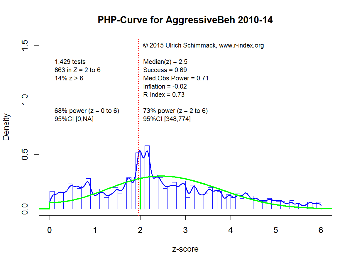
The histogram and the blue density distribution show the observed data. The green curve shows the predicted distribution based on the post-hoc power analysis. Post-hoc power analysis suggests that the average power of significant results is 67%. Power for all statistical tests is estimated to be 58% (including 11% of z-scores greater than 6, power is .58*.89 + .11 = 63%). More important is the predicted distribution of z-scores. The predicted distribution on the left side of the criterion value matches the observed distribution rather well. This shows that there are not a lot of missing non-significant results. In other words, there does not appear to be a file-drawer of studies with non-significant results. There is also only a very small blip in the observed data just at the level of statistical significance. The close match between the observed and predicted distributions suggests that results in this journal are relatively free of systematic bias due to publication bias or questionable research practices.

Example 2: A Z-Curve with Publication Bias

The second example is based on results published in the Attitudes & Social Cognition Section of the Journal of Personality and Social Psychology. The text-mining program retrieved 5,919 tests from articles published between 2010 and 2014. 3,584 tests provided z-scores in the range from 2 to 6 that is being used for model fitting.

PHP-Curve JPSP-ASC

The average power of significant results in JPSP-ASC is 55%. This is significantly less than the average power in JEP-LMC, which was used for the first example. The estimated power for all statistical tests, including those in the estimated file drawer, is 35%. More important is the estimated distribution of z-values. On the right side of the significance criterion the estimated curve shows relatively close fit to the observed distribution. This finding shows that random sampling error alone is sufficient to explain the observed distribution. However, on the left side of the distribution, the observed z-scores drop off steeply. This drop is consistent with the effect of publication bias that researchers do not report all non-significant results. There is only a slight hint that questionable research practices are also present because observed z-scores just above the criterion value are a bit more frequent than the model predicts. However, this discrepancy is not conclusive because the model could increase the file drawer, which would produce a steeper slope. The most important characteristic of this z-curve is the steep cliff on the left side of the criterion value and the gentle slope on the right side of the criterion value.

Example 3: A Z-Curve with Questionable Research Practices.

Example 3 uses results published in the journal Aggressive Behavior during the years 2010 to 2014. The text mining program found 1,429 results and 863 z-scores in the range from 2 to 6 that were used for the post-hoc-power analysis.

PHP-Curve for AggressiveBeh 2010-14


The average power for significant results in the range from 2 to 6 is 73%, which is similar to the power estimate in the first example. The power estimate that includes non-significant results is 68%. The power estimate is similar because there is no evidence of a file drawer with many underpowered studies. In fact, there are more observed non-significant results than predicted non-significant results, especially for z-scores close to zero. This outcome shows some problems of estimating the frequency of non-significant results based on the distribution of significant results. More important, the graph shows a cluster of z-scores just above and below the significance criterion. The step cliff to the left of the criterion might suggest publication bias, but the whole distribution does not show evidence of publication bias. Moreover, the steep cliff on the right side of the cluster cannot be explained with publication bias. Only questionable research practices can produce this cliff because publication bias relies on random sampling error which leads to a gentle slope of z-scores as shown in the second example.

Prevalence of Questionable Research Practices

The examples suggest that the distribution of z-scores can be used to distinguish publication bias and questionable research practices. Based on this approach, the prevalence of questionable research practices would be rare. The journal Aggressive Behavior is exceptional. Most journals show a pattern similar to Example 2, with varying sizes of the file drawer. However, this does not mean that questionable research practices are rare because it is most likely that the pattern observed in Example 2 is a combination of questionable research practices and publication bias. As shown in Example 2, the typical power of statistical tests that produce a significant result is about 60%. However, researchers do not know which experiments will produce significant results. Slight modifications in experimental procedures, so-called hidden moderators, can easily change an experiment with 60% power into an experiment with 30% power. Thus, the probability of obtaining a significant result in a replication study is less than the nominal power of 60% that is implied by post-hoc-power analysis. With only 30% to 60% power, researchers will frequently encounter results that fail to produce an expected significant result. In this case, researchers have two choices to avoid reporting a non-significant result. They can put the study in the file-drawer or they can try to salvage the study with the help of questionable research practices. It is likely that researchers will do both and that the course of action depends on the results. If the data show a trend in the right direction, questionable research practices seem an attractive alternative. If the data show a trend in the opposite direction, it is more likely that the study will be terminated and the results remain unreported.

Simons et al. (2011) conducted some simulation studies and found that even extreme use of multiple questionable research practices (p-hacking) will produce a significant result in at most 60% of cases, when the null-hypothesis is true. If such extreme use of questionable research practices were widespread, z-curve would produce corrected power estimates well-below 50%. There is no evidence that extreme use of questionable research practices is prevalent. In contrast, there is strong evidence that researchers conduct many more studies than they actually report and that many of these studies have a low probability of success.

Implications of File-Drawers for Science

First, it is clear that researchers could be more effective if they would use existing resources more effectively. An fMRI study with 20 participants costs about $10,000. Conducting a study that costs $10,000 that has only a 50% probability of producing a significant result is wasteful and should not be funded by taxpayers. Just publishing the non-significant result does not fix this problem because a non-significant result in a study with 50% power is inconclusive. Even if the predicted effect exists, one would expect a non-significant result in ever second study.   Instead of wasting $10,000 on studies with 50% power, researchers should invest $20,000 in studies with higher power (unfortunately, power does not increase proportional to resources). With the same research budget, more money would contribute to results that are being published. Thus, without spending more money, science could progress faster.

Second, higher powered studies make non-significant results more relevant. If a study had 80% power, there is only a 20% chance to get a non-significant result if an effect is present. If a study had 95% power, the chance of a non-significant result would be just as low as the chance of a false positive result. In this case, it is noteworthy that a theoretical prediction was not confirmed. In a set of high-powered studies, a post-hoc power analysis would show a bimodal distribution with clusters of z-scores around 0 for true null-hypothesis and a cluster of z-scores of 3 or higher for clear effects. Type-I and Type-II errors would be rare.

Third, Example 3 shows that the use of questionable research practices becomes detectable in the absence of a file drawer and that it would be harder to publish results that were obtained with questionable research practices.

Finally, the ability to estimate the size of file-drawers may encourage researchers to plan studies more carefully and to invest more resources into studies to keep their file drawers small because a large file-drawer may harm reputation or decrease funding.

In conclusion, post-hoc power analysis of large sets of data can be used to estimate the size of the file drawer based on the distribution of z-scores on the right side of a significance criterion. As file-drawers harm science, this tool can be used as an incentive to conduct studies that produce credible results and thus reducing the need for dishonest research practices. In this regard, the use of post-hoc power analysis complements other efforts towards open science such as preregistration and data sharing.

A Critical Review of Cumming’s (2014) New Statistics: Reselling Old Statistics as New Statistics

Cumming (2014) wrote an article “The New Statistics: Why and How” that was published in the prestigious journal Psychological Science.   On his website, Cumming uses this article to promote his book “Cumming, G. (2012). Understanding The New Statistics: Effect Sizes, Confidence Intervals, and Meta-Analysis. New York: Routledge.”

The article clear states the conflict of interest. “The author declared that he earns royalties on his book (Cumming, 2012) that is referred to in this article.” Readers are therefore warned that the article may at least inadvertently give an overly positive account of the new statistics and an overly negative account of the old statistics. After all, why would anybody buy a book about new statistics when the old statistics are working just fine.

This blog post critically examines Cumming’s claim that his “new statistics” can solve endemic problems in psychological research that have created a replication crisis and that the old statistics are the cause of this crisis.

Like many other statisticians who are using the current replication crisis as an opportunity to sell their statistical approach, Cumming’s blames null-hypothesis significance testing (NHST) for the low credibility of research articles in Psychological Science (Francis, 2013).

In a nutshell, null-hypothesis significance testing entails 5 steps. First, researchers conduct a study that yields an observed effect size. Second, the sampling error of the design is estimated. Third, the ratio of the observed effect size and sampling error (signal-to-noise ratio) is computed to create a test-statistic (t, F, chi-square). The test-statistic is then used to compute the probability of obtaining the observed test-statistic or a larger one under the assumption that the true effect size in the population is zero (there is no effect or systematic relationship). The last step is to compare the test statistic to a criterion value. If the probability (p-value) is less than a criterion value (typically 5%), the null-hypothesis is rejected and it is concluded that an effect was present.

Cumming’s (2014) claims that we need a new way to analyze data because there is “renewed recognition of the severe flaws of null-hypothesis significance testing (NHST)” (p. 7). His new statistical approach has “no place for NHST” (p. 7). His advice is to “whenever possible, avoid using statistical significance or p values” (p. 8).

So what is wrong with NHST?

The first argument against NHST is that Ioannidis (2005) wrote an influential article with the eye-catching title “Why most published research findings are false” and most research articles use NHST to draw inferences from the observed results. Thus, NHST seems to be a flawed method because it produces mostly false results. The problem with this argument is that Ioannidis (2005) did not provide empirical evidence that most research findings are false, nor is this a particularly credible claim for all areas of science that use NHST, including partical physics.

The second argument against NHST is that researchers can use questionable research practices to produce significant results. This is not really a criticism of NHST, because researchers under pressure to publish are motivated to meet any criteria that are used to select articles for publication. A simple solution to this problem would be to publish all submitted articles in a single journal. As a result, there would be no competition for limited publication space in more prestigious journals. However, better studies would be cited more often and researchers will present their results in ways that lead to more citations. It is also difficult to see how psychology can improve its credibility by lowering standards for publication. A better solution would be to ensure that researchers are honestly reporting their results and report credible evidence that can provide a solid empirical foundation for theories of human behavior.

Cummings agrees. “To ensure integrity of the literature, we must report all research conducted to a reasonable standard, and reporting must be full and accurate” (p. 9). If a researcher conducted five studies with only a 20% chance to get a significant result and would honestly report all five studies, p-values would provide meaningful evidence about the strength of the evidence, namely most p-values would be non-significant and show that the evidence is weak. Moreover, post-hoc power analysis would reveal that the studies had indeed low power to test a theoretical prediction. Thus, I agree with Cumming’s that honesty and research integrity are important, but I see no reason to abandon NHST as a systematic way to draw inferences from a sample about the population because researchers have failed to disclose non-significant results in the past.

Cumming’s then cites a chapter by Kline (2014) that “provided an excellent summary of the deep flaws in NHST and how we use it” (p. 11). Apparently, the summary is so excellent that readers are better off by reading the actual chapter because Cumming’s does not explain what these deep flaws are. He then observes that “very few defenses of NHST have been attempted” (p. 11). He doesn’t even list a single reference. Here is one by a statistician: “In defence of p-values” (Murtaugh, 2014). In a response, Gelman agrees that the problem is more with the way p-values are used rather than with the p-value and NHST per se.

Cumming’s then states a single problem of NHST. Namely that it forces researchers to make a dichotomous decision. If the signal-to-noise ratio is above a criterion value, the null-hypothesis is rejected and it is concluded that an effect is present. If the signal-to-noise ratio is below the criterion value the null-hypothesis is not rejected. If Cumming’s has a problem with decision making, it would be possible to simply report the signal-to-noise ratio or simply to report the effect size that was observed in a sample. For example, mortality in an experimental Ebola drug trial was 90% in the control condition and 80% in the experimental condition. As this is the only evidence, it is not necessary to compute sampling error, signal-to-noise ratios, or p-values. Given all of the available evidence, the drug seems to improve survival rates. But wait. Now a dichotomous decision is made based on the observed mean difference and there is no information about the probability that the results in the drug trial generalize to the population. Maybe the finding was a chance finding and the drug actually increases mortality. Should we really make life-and-death decision if the decision were based on the fact that 8 out of 10 patients died in one condition and 9 out of 10 patients died in the other condition?

Even in a theoretical research context decisions have to be made. Editors need to decide whether they accept or reject a submitted manuscript and readers of published studies need to decide whether they want to incorporate new theoretical claims in their theories or whether they want to conduct follow-up studies that build on a published finding. It may not be helpful to have a fixed 5% criterion, but some objective information about the probability of drawing the right or wrong conclusions seems useful.

Based on this rather unconvincing critique of p-values, Cumming’s (2014) recommends that “the best policy is, whenever possible, not to use NHST at all” (p. 12).

So what is better than NHST?

Cumming then explains how his new statistics overcome the flaws of NHST. The solution is simple. What is astonishing about this new statistic is that it uses the exact same components as NHST, namely the observed effect size and sampling error.

NHST uses the ratio of the effect size and sampling error. When the ratio reaches a value of 2, p-values reach the criterion value of .05 and are considered sufficient to reject the null-hypothesis.

The new statistical approach is to multiple the standard error by a factor of 2 and to add and subtract this value from the observed mean. The interval from the lower value to the higher value is called a confidence interval. The factor of 2 was chosen to obtain a 95% confidence interval.  However, drawing a confidence interval alone is not sufficient to draw conclusions from the data. Whether we describe the results in terms of a ratio, .5/.2 = 2.5 or in terms of a 95%CI = .5 +/- .2 or CI = .1 to .7, is not a qualitative difference. It is simply different ways to provide information about the effect size and sampling error. Moreover, it is arbitrary to multiply the standard error by a factor of 2. It would also be possible to multiply it by a factor of 1, 3, or 5. A factor of 2 is used to obtain a 95% confidence interval rather than a 20%, 50%, 80%, or 99% confidence interval. A 95% confidence is commonly used because it corresponds to a 5% error rate (100 – 95 = 5!). A 95% confidence interval is as arbitrary as a p-value of .05.

So, how can a p-value be fundamentally wrong and how can a confidence interval be the solution to all problems if they provide the same information about effect size and sampling error? In particular how do confidence intervals solve the main problem of making inferences from an observed mean in a sample about the mean in a population?

To sell confidence intervals, Cumming’s uses a seductive example.

“I suggest that, once freed from the requirement to report p values, we may appreciate how simple, natural, and informative it is to report that “support for Proposition X is 53%, with a 95% CI of [51, 55],” and then interpret those point and interval estimates in practical terms” (p 14).

Support for proposition X is a rather unusual dependent variable in psychology. However, let us assume that Cumming refers to an opinion poll among psychologists whether NHST should be abandoned. The response format is a simple yes/no format. The average in the sample is 53%. The null-hypothesis is 50%. The observed mean of 53% in the sample shows more responses in favor of the proposition. To compute a significance test or to compute a confidence interval, we need to know the standard error. The confidence interval ranges from 51% to 55%. As the 95% confidence interval is defined by the observed mean plus/minus two standard errors, it is easy to see that the standard error is SE = (53-51)/2 = 1% or .01. The formula for the standard error in a one sample test with a dichotomous dependent variable is sqrt(p * (p-1) / n)). Solving for n yields a sample size of N = 2,491. This is not surprising because public opinion polls often use large samples to predict election outcomes because small samples would not be informative. Thus, Cumming’s example shows how easy it is to draw inferences from confidence intervals when sample sizes are large and confidence intervals are tight. However, it is unrealistic to assume that psychologists can and will conduct every study with samples of N = 1,000. Thus, the real question is how useful confidence intervals are in a typical research context, when researchers do not have sufficient resources to collect data from hundreds of participants for a single hypothesis test.

For example, sampling error for a between-subject design with N = 100 (n = 50 per cell) is SE = 2 / sqrt(100) = .2. Thus, the lower and upper limit of the 95%CI are 4/10 of a standard deviation away from the observed mean and the full width of the confidence interval covers 8/10th of a standard deviation. If the true effect size is small to moderate (d = .3) and a researcher happens to obtain the true effect size in a sample, the confidence interval would range from d = -.1 to d = .7. Does this result support the presence of a positive effect in the population? Should this finding be published? Should this finding be reported in newspaper articles as evidence for a positive effect? To answer this question, it is necessary to have a decision criterion.

One way to answer this question is to compute the signal-to-noise ratio, .3/.2 = 1.5 and to compute the probability that the positive effect in the sample could have occurred just by chance, t(98) = .3/.2 = 1.5, p = .15 (two-tailed). Given this probability, we might want to see stronger evidence. Moreover, a researcher is unlikely to be happy with this result. Evidently, it would have been better to conduct a study that could have provided stronger evidence for the predicted effect, say a confidence interval of d = .25 to .35, but that would have required a sample size of N = 6,500 participants.

A wide confidence interval can also suggest that more evidence is needed, but the important question is how much more evidence is needed and how narrow a confidence interval should be before it can give confidence in a result. NHST provides a simple answer to this question. The evidence should be strong enough to reject the null-hypothesis with a specified error rate. Cumming’s new statistics provides no answer to the important question. The new statistics is descriptive, whereas NHST is an inferential statistic. As long as researchers merely want to describe their data, they can report their results in several ways, including reporting of confidence intervals, but when they want to draw conclusions from their data to support theoretical claims, it is necessary to specify what information constitutes sufficient empirical evidence.

One solution to this dilemma is to use confidence intervals to test the null-hypothesis. If the 95% confidence interval does not include 0, the ratio of effect size / sampling error is greater than 2 and the p-value would be less than .05. This is the main reason why many statistics programs report 95%CI intervals rather than 33%CI or 66%CI. However, the use of 95% confidence intervals to test significance is hardly a new statistical approach that justifies the proclamation of a new statistic that will save empirical scientists from NHST. It is NHST! Not surprisingly, Cumming’s states that “this is my least preferred way to interpret a confidence interval” (p. 17).

However, he does not explain how researchers should interpret a 95% confidence interval that does include zero. Instead, he thinks it is not necessary to make a decision. “We should not lapse back into dichotomous thinking by attaching any particular importance to whether a value of interest lies just inside or just outside our CI.”

Does an experimental treatment for Ebolay work? CI = -.3 to .8. Let’s try it. Let’s do nothing and do more studies forever. The benefit of avoiding making any decisions is that one can never make a mistake. The cost is that one can also never claim that an empirical claim is supported by evidence. Anybody who is worried about dichotomous thinking might ponder the fact that modern information processing is built on the simple dichotomy of 0/1 bits of information and that it is common practice to decide the fate of undergraduate students on the basis of scoring multiple choice tests in terms of True or False answers.

In my opinion, the solution to the credibility crisis in psychology is not to move away from dichotomous thinking, but to obtain better data that provide more conclusive evidence about theoretical predictions and a simple solution to this problem is to reduce sampling error. As sampling error decreases, confidence intervals get smaller and are less likely to include zero when an effect is present and the signal-to-noise ratio increases so that p-values get smaller and smaller when an effect is present. Thus, less sampling error also means less decision errors.

The question is how small should sampling error be to reduce decision error and at what point are resources being wasted because the signal-to-noise ratio is clear enough to make a decision.

Power Analysis

Cumming’s does not distinguish between Fischer’s and Neyman-Pearson’s use of p-values. The main difference is that Fischer advocated the use of p-values without strict criterion values for significance testing. This approach would treat p-values just like confidence intervals as continuous statistics that do not imply an inference. A p-value of .03 is significant with a criterion value of .05, but it is not significant with a criterion value of .01.

Neyman-Pearson introduced the concept of a fixed criterion value to draw conclusions from observed data. A criterion value of p = .05 has a clear interpretation. It means that a test of 1,000 null-hypotheses is expected to produce about 50 significant results (type-I errors). A lower error rate can be achieved by lowering the criterion value (p < .01 or p < .001).

Importantly, Neyman-Pearson also considered the alternative problem that the p-value may fail to reach the critical value when an effect is actually present. They called this probability the type-II error. Unfortunately, social scientists have ignored this aspect of Neyman-Pearson Significance Testing (NPST). Researchers can avoid making type-II errors by reducing sampling error. The reason is that a reduction of sampling error increases the signal-to-noise ratio.

For example, the following p-values were obtained from simulating studies with 95% power. The graph only shows p-values greater than .001 to make the distribution of p-values more prominent. As a result 62.5% of the data are missing because these p-values are below p < .001. The histogram of p-values has been popularized by Simmonsohn et al. (2013) as a p-curve. The p-curve shows that p-values are heavily skewed towards low p-values. Thus, the studies provide consistent evidence that an effect is present, even though p-values can vary dramatically from one study (p = .0001) to the next (p = .02). The variability of p-values is not a problem for NPST as long as the p-values lead to the same conclusion because the magnitude of a p-value is not important in Neyman-Pearson hypothesis testing.

CumFig1

The next graph shows p-values for studies with 20% power. P-values vary just as much, but now the variation covers both sides of the significance criterion, p = .05. As a result, the evidence is often inconclusive and 80% of studies fail to reject the false null-hypothesis.

CumFig2

R-Code
seed = length(“Cumming’sDancingP-Values”)
power=.20
low_limit = .000
up_limit = .10
p <-(1-pnorm(rnorm(2500,qnorm(.975,0,1)+qnorm(.20,0,1),1),0,1))*2
hist(p,breaks=1000,freq=F,ylim=c(0,100),xlim=c(low_limit,up_limit))
abline(v=.05,col=”red”)
percent_below_lower_limit = length(subset(p, p <  low_limit))/length(p)
percent_below_lower_limit
If a study is designed to test a qualitative prediction (an experimental manipulation leads to an increase on an observed measure), power analysis can be used to plan a study so that it has a high probability of providing evidence for the hypothesis if the hypothesis is true. It does not matter whether the hypothesis is tested with p-values or with confidence intervals by showing that the confidence does not include zero.

Thus, power analysis seems useful even for the new statistics. However, Cummings is “ambivalent about statistical power” (p. 23). First, he argues that it has “no place when we use the new statistics” (p. 23), presumably because the new statistics never make dichotomous decisions.

Cumming’s next argument against power is that power is a function of the type-I error criterion. If the type-I error probability is set to 5% and power is only 33% (e.g., d = .5, between-group design N = 40), it is possible to increase power by increasing the type-I error probability. If type-I error rate is set to 50%, power is 80%. Cumming’s thinks that this is an argument against power as a statistical concept, but raising alpha to 50% is equivalent to reducing the width of the confidence interval by computing a 50% confidence interval rather than a 95% confidence interval. Moreover, researchers who adjust alpha to 50% are essentially saying that the null-hypothesis would produce a significant result in every other study. If an editor finds this acceptable and wants to publish the results, neither power analysis nor the reported results are problematic. It is true that there was a good chance to get a significant result when a moderate effect is present (d = .5, 80% probability) and when no effect is present (d = 0, 50% probability). Power analysis provides accurate information about the type-I and type-II error rates. In contrast, the new statistics provides no information about error rates in decision making because it is merely descriptive and does not make decisions.

Cumming then points out that “power calculations have traditionally been expected [by granting agencies], but these can be fudged” (p. 23). The problem with fudging power analysis is that the requested grant money may be sufficient to conduct the study, but insufficient to produce a significant result. For example, a researcher may be optimistic and expect a strong effect, d = .80, when the true effect size is only a small effect, d = .20. The researcher conducts a study with N = 52 participants to achieve 80% power. In reality the study has only 11% power and the researcher is likely to end up with a non-significant result. In the new statistics world this is apparently not a problem because the researcher can report the results with a wide confidence interval that includes zero, but it is not clear why a granting agency should fund studies that cannot even provide information about the direction of an effect in the population.

Cummings then points out that “one problem is that we never know true power, the probability that our experiment will yield a statistically significant result, because we do not know the true effect size; that is why we are doing the experiment!” (p. 24). The exclamation mark indicates that this is the final dagger in the coffin of power analysis. Power analysis is useless because it makes assumptions about effect sizes when we can just do an experiment to observe the effect size. It is that easy in the world of new statistics. The problem is that we do not know the true effect sizes after an experiment either. We never know the true effect size because we can never determine a population parameter, just like we can never prove the null-hypothesis. It is only possible to estimate population parameter. However, before we estimate a population parameter, we may simply want to know whether an effect exists at all. Power analysis can help in planning studies so that the sample mean shows the same sign as the population mean with a specified error rate.

Determining Sample Sizes in the New Statistics

Although Cumming does not find power analysis useful, he gives some information about sample sizes. Studies should be planned to have a specified level of precision. Cumming gives an example for a between-subject design with n = 50 per cell (N = 100). He chose to present confidence intervals for unstandardized coefficients. In this case, there is no fixed value for the width of the confidence interval because the sampling variance influences the standard error. However, for standardized coefficients like Cohen’s d, sampling variance will produce variation in standardized coefficients, while the standard error is constant. The standard error is simply 2 / sqrt (N), which equals SE = .2 for N = 100. This value needs to be multiplied by 2 to get the confidence interval, and the 95%CI = d +/- .4.   Thus, it is known before the study is conducted that the confidence interval will span 8/10 of a standard deviation and that an observed effect size of d > .4 is needed to exclude 0 from the confidence interval and to state with 95% confidence that the observed effect size would not have occurred if the true effect size were 0 or in the opposite direction.

The problem is that Cumming provides no guidelines about the level of precision that a researcher should achieve. Is 8/10 of a standard deviation precise enough? Should researchers aim for 1/10 of a standard deviation? So when he suggests that funding agencies should focus on precision, it is not clear what criterion should be used to fund research.

One obvious criterion would be to ensure that precision is sufficient to exclude zero so that the results can be used to state that direction of the observed effect is the same as the direction of the effect in the population that a researcher wants to generalize to. However, as soon as effect sizes are used in the planning of the precision of a study, precision planning is equivalent to power analysis. Thus, the main novel aspect of the new statistics is to ignore effect sizes in the planning of studies, but without providing guidelines about desirable levels of precision. Researchers should be aware that N = 100 in a between-subject design gives a confidence interval that spans 8/10 of a standard deviation. Is that precise enough?

Problem of Questionable Research Practices, Publication Bias, and Multiple Testing

A major problem for any statistical method is the assumption that random sampling error is the only source of error. However, the current replication crisis has demonstrated that reported results are also systematically biased. A major challenge for any statistical approach, old or new, is to deal effectively with systematically biased data.

It is impossible to detect bias in a single study. However, when more than one study is available, it becomes possible to examine whether the reported data are consistent with the statistical assumption that each sample is an independent sample and that the results in each sample are a function of the true effect size and random sampling error. In other words, there is no systematic error that biases the results. Numerous statistical methods have been developed to examine whether data are biased or not.

Cumming (2014) does not mention a single method for detecting bias (Funnel Plot, Eggert regression, Test of Excessive Significance, Incredibility-Index, P-Curve, Test of Insufficient Variance, Replicabiity-Index, P-Uniform). He merely mentions a visual inspection of forest plots and suggests that “if for example, a set of studies is distinctly too homogeneous – it shows distinctly less bouncing around than we would expect from sampling variability… we can suspect selection or distortion of some kind” (p. 23). However, he provides no criteria that explain how variability of observed effect sizes should be compared against predicted variability and how the presence of bias influences the interpretation of a meta-analysis. Thus, he concludes that “even so [biases may exist], meta-analysis can give the best estimates justified by research to date, as well as the best guidance for practitioners” (p. 23). Thus, the new statistics would suggest that extrasensory perception is real because a meta-analysis of Bem’s (2011) infamous Journal of Personality and Social Psychology article shows an effect with a tight confidence interval that does not include zero. In contrast, other researchers have demonstrated with old statistical tools and with the help of post-hoc power that Bem’s results are not credible (Francis, 2012; Schimmack, 2012).

Research Integrity

Cumming also advocates research integrity. His first point is that psychological science should “promote research integrity: (a) a public research literature that is complete and trustworthy and (b) ethical practice, including full and accurate reporting of research” (p. 8). However, his own article falls short of this ideal. His article does not provide a complete, balanced, and objective account of the statistical literature. Rather, Cumming (2014) cheery-picks references that support his claims and does not cite references that are inconvenient for his claims. I give one clear example of bias in his literature review.

He cites Ioannidis’s 2005 paper to argue that p-values and NHST is flawed and should be abandoned. However, he does not cite Ioannidis and Trikalinos (2007). This article introduces a statistical approach that can detect biases in meta-analysis by comparing the success rate (percentage of significant results) to the observed power of the studies. As power determines the success rate in an honest set of studies, a higher success rate reveals publication bias. Cumming not only fails to mention this article. He goes on to warn readers “beware of any power statement that does not state an ES; do not use post hoc power.” Without further elaboration, this would imply that readers should ignore evidence for bias with the Test of Excessive Significance because it relies on post-hoc power. To support this claim, he cites Hoenig and Heisey (2001) to claim that “post hoc power can often take almost any value, so it is likely to be misleading” (p. 24). This statement is misleading because post-hoc power is no different from any other statistic that is influenced by sampling error. In fact,Hoenig and Heisey (2001) show that post-hoc power in a single study is monotonically related to p-values. Their main point is that post-hoc power provides no other information than p-values. However, like p-values, post-hoc power becomes more informative, the higher it is. A study with 99% post-hoc power is likely to be a high powered study, just like extremely low p-values, p < .0001, are unlikely to be obtained in low powered studies or in studies when the null-hypothesis is true. So, post-hoc power is informative when it is high. Cumming (2014) further ignores that variability of post-hoc power estimates decreases in a meta-analysis of post-hoc power and that post-hoc power has been used successfully to reveal bias in published articles (Francis, 2012; Schimmack (2012). Thus, his statement that researchers should ignore post-hoc power analyses is not supported by an unbiased review of the literature, and his article does not provide a complete and trustworthy account of the public research literature.

Conclusion

I cannot recommend Cumming’s new statistics. I routinely report confidence intervals in my empirical articles, but I do not consider them as a new statistical tool. In my opinion, the root cause of the credibility crisis is that researchers conduct underpowered studies that have a low chance to produce the predicted effect and then use questionable research practices to boost power and to hide non-significant results that could not be salvaged. A simple solution to this problem is to conduct more powerful studies that can produce significant results when the predict effect exists. I do not claim that this is a new insight. Rather, Jacob Cohen has tried his whole life to educate psychologists about the importance of statistical power.

Here is what Jacob Cohen had to say about the new statistics in 1994 using time-travel to comment on Cumming’s article 20 years later.

“Everyone knows” that confidence intervals contain all the information to be found in significance tests and much more. They not only reveal the status of the trivial nil hypothesis but also about the status of non-nil null hypotheses and thus help remind researchers about the possible operation of the crud factor. Yet they are rarely to be found in the literature. I suspect that the main reason they are not reported is that they are so embarrassingly large! But their sheer size should move us toward improving our measurement by seeking to reduce the unreliable and invalid part of the variance in our measures (as Student himself recommended almost a century ago). Also, their width provides us with the analogue of power analysis in significance testing—larger sample sizes reduce the size of confidence intervals as they increase the statistical power of NHST” (p. 1002).

If you are looking for a book on statistics, I recommend Cohen’s old statistics over Cumming’s new statistics, p < .05.

Conflict of Interest: I do not have a book to sell (yet), but I strongly believe that power analysis is an important tool for all scientists who have to deal with uncontrollable variance in their data. Therefore I am strongly opposed to Cumming’s push for a new statistics that provides no guidelines for researchers how they can optimize the use of their resources to obtain credible evidence for effects that actually exist and no guidelines how science can correct false positive results.

The Replicability-Index (R-Index): Quantifying Research Integrity

ANNIVERSARY POST.  Slightly edited version of first R-Index Blog on December 1, 2014.

In a now infamous article, Bem (2011) produced 9 (out of 10) statistically significant results that appeared to show time-reversed causality.  Not surprisingly, subsequent studies failed to replicate this finding.  Although Bem never admitted it, it is likely that he used questionable research practices to produce his results. That is, he did not just run 10 studies and found 9 significant results. He may have dropped failed studies, deleted outliers, etc.  It is well-known among scientists (but not lay people) that researchers routinely use these questionable practices to produce results that advance their careers.  Think, doping for scientists.

I have developed a statistical index that tracks whether published results were obtained by conducting a series of studies with a good chance of producing a positive result (high statistical power) or whether researchers used questionable research practices.  The R-Index is a function of the observed power in a set of studies. More power means that results are likely to replicate in a replication attempt.  The second component of the R-index is the discrepancy between observed power and the rate of significant results. 100 studies with 80% power should produce, on average, 80% significant results. If observed power is 80% and the success rate is 100%, questionable research practices were used to obtain more significant results than the data justify.  In this case, the actual power is less than 80% because questionable research practices inflate observed power. The R-index subtracts the discrepancy (in this case 20% too many significant results) from observed power to adjust for the inflation.  For example, if observed power is 80% and success rate is 100%, the discrepancy is 20% and the R-index is 60%.

In a paper, I show that the R-index predicts success in empirical replication studies.

The R-index also sheds light on the recent controversy about failed replications in psychology (repligate) between replicators and “replihaters.”   Replicators sometimes imply that failed replications are to be expected because original studies used small samples with surprisingly large effects, possibly due to the use of questionable research practices. Replihaters counter that replicators are incompetent researchers who are motivated to produce failed studies.  The R-Index makes it possible to evaluate these claims objectively and scientifically.  It shows that the rampant use of questionable research practices in original studies makes it extremely likely that replication studies will fail.  Replihaters should take note that questionable research practices can be detected and that many failed replications are predicted by low statistical power in original articles.