There are many statistical approaches that are often divided into three schools of thought: (a) Fisherian, (b) Neyman-Pearsonion, and (c) Bayesian.  This post is about Bayesian statistics.  Within Bayesian statistics, there are further distinctions that can be made. One distinction is between Bayesian parameter estimation (credibility intervals) and Bayesian hypothesis testing.  This post is about Bayesian hypothesis testing.  One goal of As one goal of Bayesian Hypothesis testing is to provide evidence for the null-hypothesis.  It is often argued that Baysian Null-Hypothesis Testing (BNHT) is superior to the widely used method of Null-Hypothesis Testing with p-values.  This post is about the ability of BNHT to test the null-hypothesis.

The crucial idea of BNHT is that it is possible to contrast the null-hypothesis (H0) with an alternative hypothesis (H1) and to compute the relative likelihood that the data support one hypothesis versus the other:  p(H0/D) / p(H1/D).  If this ratio is large enough (e.g, p(H0/D) / p(H1/D) > criterion),  it can be stated that the data support the null-hypothesis more than the alternative hypothesis.

To compute the ratio of the two conditional probabilities, researchers need to quantify two ratios.  One ratio is the prior ratio of the probabilities that H0 or H1 are true: p(H0)/p(H1. This ratio does not have a common name. I call it the probability ratio (PR).  The other ratio is the ratio of the conditional probabilities of the data given H0 and H1. This ratio is often called a Bayes Factor (BF): BF = p(D/H0)/p(D/H1).

To make claims about H0 and H1 based on some observed test statistic,  the Probability Ratio has to be multiplied with the Bayes Factor.

p(H0/D)                 p(H0)   x  p(D/H0)
________   =   _______________     =   PR * BF
p(H1/D)                  p(H1)   x   p(D/H1)
The main reason for calling this approach Bayesian is that Bayesian statisticians are willing and required to specify a priori probabilties of hypotheses before any data are collected.  In the formula above, p(H0) and p(H1) are the a priori probabilities that a population effect size is 0 (p(H0) or that it is some other value, p(H1).  However, in practice BNHT is often used without specifying these a priori probabilities.

“Table 1 provides critical t values needed for JZS Bayes factor values of 1/10, 1/3, 3, and 10 as a function of sample size. This table is analogous in form to conventional t-value tables for given p value criteria. For instance, suppose a researcher observes a t value of 3.3 for 100 observations. This t value favors the alternative and corresponds to a JZS Bayes factor less than 1/10 because it exceeds the critical value of 3.2 reported in the table. Likewise,
suppose a researcher observes a t value of 0.5. The corresponding JZS Bayes factor is greater than 10 because the t value is smaller than 0.69, the corresponding critical value in Table 1. Because the Bayes factor is directly interpretable as an odds ratio, it may be reported without reference to cutoffs such as 3 or 1/10. Readers may decide the meaning of odds ratios for themselves” (Rouder et al., 2009).

The use of arbitrary cutoff values (3 or 10) for Bayes Factors is not a complete Bayesian statistical analysis because it does not provide information about the hypothesis given the data. Bayes Factors alone only provide information about the ratio of the conditional probabilities of the data given two alternative hypothesis and the ratios are not equivalent.

p(H0/D)                 p(D/H0)
________   ≠   _________
p(H1/D)                  p(D/H1)

In practice, users of BNHT are unaware or ignore the need to think about the base rates of H0 and H1, when they interpret Bayes Factors.  The main point of this post is to demonstrate that Bayes Factors that compare the null-hypothesis of a single effect size against an alternative hypothesis that combines many effect sizes (all effect sizes that are not zero) can be deceptive because the ratio of p(H0) / p(H1) decreases as the number of effect sizes increases.  In the limit the a priori probability of the null-hypothesis being true is zero, which implies that no data can provide evidence for it because any Bayes-Factor that is multiplied with zero is zero, which implies that it is reasonable to believe in the alternative hypothesis no matter how strongly a Bayes Factor favors the null-hypothesis.

The following urn experiments explains the logic of my argument, points out a similar problem in the famous Monty Hall problem, and provides r-code to run simulations with different assumptions about the number and distribution of effect sizes and the implications for the probability ratio of H0 and H1 and Bayes Factors that are need to provide evidence for the null-hypothesis.

An Urn Experiment of Population Effect Sizes

The classic example in statistics are urn experiments.  An urn is filled with balls with different colors. If the urn is filled with 100 balls and only one ball is red and you get one chance to draw a ball from the urn without peeking, the probability of you drawing the red ball is 1 out of 100 or 1%.

To think straight about statistics and probabilities it is helpful, unless you are some math genius who can really think in 10 dimensions, to remind yourself that even complicated probability problems are essentially urn experiments. The question is only what the urn experiment would look like.

In this post, I am examining the urn experiment that corresponds to the problem of Bayesian statisticians to specify probabilities of effect sizes in experiments without any information that would be helpful to guess which effect size is most likely.

To translate the Bayesian problem of the prior into an urn experiment, we first have to turn effect sizes into balls.  The problem is that effect sizes are typically continuous, but an urn can only be filled with discrete objects.  The solution to this problem is to cut the continuous range of effect sizes into discrete units.  The number of units depends on the desired precision.  For example, effect sizes can be measured in standardized units with one decimal, d = 0, d = .1, d = .2, etc.  or with two decimals, d = .00, d = .01, d = .02, etc.  or with 10 decimals.  The more precise the measurement, the more discrete events are created.  Instead of using colors, we can use balls with numbers printed on them as you may have seen in lottery draws.   In psychology, theories and empirical studies often are not very precise and it would hardly be meaningful to distinguish between an effect size of d = .213 and an effect size of d = .214.  Even two decimals are rarely needed and the typical sampling error in psychological studies of d = .20, would make it impossible to distinguish between d = .33 and d = .38 empirically.  So, it makes sense to translate the continuous range of effect sizes into balls with one digit numbers, d = .0, d = .1, d = .2.

The second problem is that effect sizes can be positive or negative.  This is not really a problem because some balls can have negative numbers printed on them.  However, the example can be generalized from the one-sided scenario with only positive effect sizes to a two-sided scenario that also includes negative effects. To keep things simple, I use only positive effect sizes in this example.

The third problem is that some effect size measures are unlimited. However, in practice it is unreasonable to expect very large effect sizes and it is possible to limit the range of possible effect sizes at a maximum value.  The limit could be d = 10, d = 5, or d = 2.  For this example, I use a limit of d = 2.

It is now possible to translate the continuous measure of standardized effect sizes into 21 discrete events and to fill the urn with 21 balls that have printed the numbers 0, 0.1, 0.2, …., 2.0 printed on them.

The main point of Bayesian inference is to draw conclusions about the probability that a particular hypothesis is true given the results of an empirical study.  For example, how probable is it that the null-hypothesis is true when I observe an effect size of d = .2?  However, a study only provides information about the data given a specific hypothesis. How probable is it to observe an effect size of d = .2, if the null-hypothesis were true?  To answer the first question, it is necessary to specify the probability that the hypothesis is true independent of any data; that is, how probable is it that the null-hypothesis is true?

P(pop.es=0/obs.es = .2) = P(pop.es=0) * P(Obs.ES=.2/Pop.ES=0) / P(Obs.ES = .20)

This looks scary and for this post you do not need to understand the complete formula ,but it is just a mathematical way of saying that the probability that a population effect size (pop.es) is zero when the observed effect size (obs.es) is d = .2 equals the unconditional probability that the population effect size is zero multiplied by the conditional probability of observing an effect size of d = .2 when the population effect size is 0 divided by the unconditional probability of observing an effect size of d = .2.

I only show this formula to highlight the fact that the main goal of Bayesian inference is to estimate the probability of a hypothesis (in this case, pop.es = 0) given some observed data (in this case, obs.es = .20) and that researchers need to specify the unconditional probability of the hypothesis (pop.es = 0) to do so.

We can now return to the urn experiment and ask the question how likely it is that a particular hypothesis is true. For example, how likely is it that the null-hypothesis is true?  That is, how likely is it that we end up with a ball that has the number 0.0 printed on it when conduct a study with an unknown population effect size? The answer is: it depends.  It depends on the way our urn was filled.  We of course do not know how often the null-hypothesis is true, but we can fill the urn in a way that expresses maximum uncertainty about the probability that the null-hypothesis is true.  Maximum uncertainty means that all possible events are equally likely (Bayesian statisticians actually use a so-called uniform prior when the range of possible outcomes is fixed).  So, we can fill the urn with one ball for each of the 21 effect sizes (0.0, 0.1, 0.2,….. 2.0).   Now it is fairly easy to determine the a priori probability that the null-hypothesis is true.  There are 21 balls and you are drawing one ball from the urn.  Thus, the a priori probability of the null-hypothesis being true is 1/21 = .047.

As noted before, if the range of events increases because we specify a wider range of effect sizes (say effect sizes up to 10), the a priori probability of drawing the ball with 0.0 printed on it decreases. If we specify effect sizes with more precision (e.g., two digits), the probability of drawing the ball that has 0.00 printed on it decreases further.  With effect sizes ranging from 0 to 10 and being specified with two digits, there are 1001 balls in the urn and the probability of drawing the ball with 0.00 printed on it is 0.001.  Thus, even if the data would provide strong support for the null-hypothesis, the proper inference has to take into account that a priori it is very unlikely that a randomly drawn study had an effect size of 0.00.

As effect sizes are continuous and theoretically can range from -infinity to +infinity, there is an infinite number of effect sizes and the probability of drawing a ball with 0 printed on it from an infinitely large urn that is filled with an infinite number of balls is zero (1/infinity).  This would suggest that it is meaningless to test the hypothesis whether the null-hypothesis is true or not because we already know the answer to the question; the probability is zero. As any number that is multiplied by 0 is zero, the probability that the population effect size is zero remains zero, even if the probability that the population effect size is 0 when we observed an effect size of 0 is 1.   Of course, this is also true for any other hypothesis about effect sizes greater than zero. The probability that the effect size is exactly d = .2 is also 0.  The implication is simply that it is not possible to empirically test hypotheses when the range of effect sizes is cut into an infinite number of pieces because the a priori probability that the effect size has a specific size is always 0.   This problem can be solved by limiting the number of balls in the urn so that we avoid the problem of drawing from an infinitely large urn with an infinite number of balls.

Bayesians solve the infinity problem by using mathematical functions.  A commonly used function was proposed by Jeffrey’s.  Jeffrey’s proposed to specify uncertainty about effect sizes with a Cauchy distribution with a scaling parameter of 1.  Figure 1 shows the distribution.

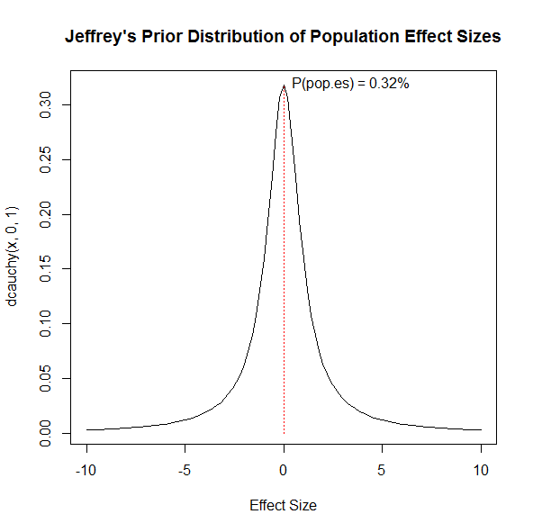
The figure is cut off at effect sizes smaller than -10 and larger than 10, and it assumes that effect sizes are measured with two digits.  With two decimals, the densities can be interpreted as percentages and sum to 100.  The sum of the probabilities for effect sizes in the range between -10 and 10 covers only 93.66% of the full distribution. The remaining 6.34% are in the tails below -10 and above 10. As you can see, the distribution is not uniform. It actually gives the highest probability to an effect size of 0. The probability density for an effect size of 0 is 0.32 and translates into a probability of 0.32% with two digits as units for the effect size.   By eliminating these extreme effect sizes, the probability of the null-hypothesis increases slightly from 0.32% to 0.32/93.66*100 = 0.34%. With two decimals, there are 2001 effect sizes (-10, -9.99, …..-0.01, 0, 0.1….,9.99,10). A uniform prior would put the probability of a single effect size at 1/2001 = 0.05%.  This shows that Jeffrey’s prior gives a higher probability to the null-hypothesis, but it also does so for other small effect sizes close to zero.  The probability density of observing an effect size of d = 0.01 is only slightly smaller, d = .31827, than the probability of the null-hypothesis, d = .3183.

If we translate Jeffrey’s prior for effect sizes with two digits into an urn experiment, and we filled the urn proportionally to the distribution in Figure 1 with 10,000 balls, 34 balls would have the number 0.00 printed on them.  When we draw one ball from the urn, the probability of drawing one of the 34 balls with 0.00, is 34/10000 = 0.0034 or 0.34%.

Bayesian statisticians do not use probability densities to specify the probability that the population effect size is zero, possibly because probability densities do not directly translate into probabilities and the unit.  However, by treating effect sizes as a continuous variable, the number of balls in the lottery is infinite and the probability of drawing a ball with 0.0000000000000000 printed on it is practically zero.  A reasonable alternative is to specify a reasonable unit for effect sizes.  As noted earlier, for many psychological applications, a reasonable unit is a single digit (d = 0, d = .1, d = .2, etc.).  This implies that effect sizes between d = -.05 and d = .05 are essentially treated as 0.

Given Jeffrey’s distribution, the rational specification of the a prior probabilities that the effect size is 0 or somewhere between -10 and 10 is

P(pop.es = 0)                      0.32                                     1
___________   =    _____________      =    ______

P(pop.es ≠ 0)                   9.37 – 0.32                           28
To draw statistical inferences Bayesian Null Hypothesis Tests uses the Bayes-Factor.  Without going into details here, a Bayes-Factor provides the complementary ratio of the conditional probabilities of data based on the null-hypothesis or the alternative hypothesis.  It is not uncommon to use a Bayes-Factor of 3 or greater as support for one of the two hypotheses.  However, if we take the prior probabilities of these hypothesis into account a Bayes-Factor of 3 does not justify a belief in the null-hypothesis, nor is it sufficiently strong to overcome the low probability that the null-hypothesis is true given the large uncertainty about effect sizes. A Bayes-Factor of 3 would change the probability of 1/28 into a probability of 3/28 = .11.  Thus, it is still unlikely that the effect size is zero.  A Bayes-Factor of 28 in favor of H0, would be needed to make it equally likely that the null-hypothesis is true and that it is not true and to assert that the null-hypothesis is true with a probability of 90%, the Bayes-Factor would have to be 255; 255/28 = 9 = .90/.10.

It is possible to further decrease the number of balls in the lottery. For example, it is possible to set the unit to 1. This gives only 11 effect sizes (-10, -9, -8,…,-1,0,1,…8,9,10).  The probability density of .32 translates now in a .32 probability, versus a .68 probability for all other effect sizes. After adjusting for the range restriction, this translates into a ratio of 1.95 to 1 in favor of the alternative.  Thus, a Bayes-Factor of 3 would favor the null-hypothesis and it would only require a Bayes-Factor of 18 to obtain a probability of .90 that H0 is true,  18/1.95 = 9 = .90/.10.   However, it is important to realize that the null-hypothesis with d = 1 covers effect sizes in the range from -.5 to .5.   This wide range covers effect sizes that are typical for psychology and are commonly called small or moderate effects.  As a result, this is not a practical solution because the test no longer really tests the hypothesis that there is no effect.

In conclusion, Jeffrey’s proposed a rational approach to specify the probability of population effect sizes without any data and without prior information about effect sizes.  He proposed a prior distribution of population effect sizes that covers a wide range of effect sizes.  The cost of working with this prior distribution of effect sizes under maximum uncertainty is that a wide range of effect sizes are considered to be plausible. This means that there are many possible events and the probability of any single event is small.  Jeffrey’s prior makes it possible to quantify this probability as a function of the density of an effect size and the precision of measurement of effect sizes (number of digits).  This probability should be used to evaluate Bayes-Factors.  Contrary to existing norms, Bayes-Factors of 3 or 10 cannot be used to claim that the data favor the null-hypothesis over the alternative hypothesis because this interpretation of Bayes-Factors ignore that without further information it is more likely that the null-hypothesis is false than that it is correct.   It seems unreasonable to assign equal probabilities to two events, where one event is akin to drawing a single red ball from an urn when the other event is to draw all but that red ball from an urn.  As the number of balls in the urn increases, these probabilities become more and more unequal.  Any claim that the null-hypothesis is equally or more probable than other effects would have to be motivated by prior information, which would invalidate the use of Jeffrey’s distribution of effect sizes that was developed for a scenario where prior information is not available.

Postscript or Part II

One of the most famous urn experiments in probability theory is the Monty Hall problem.

Suppose you’re on a game show, and you’re given the choice of three doors: Behind one door is a car; behind the others, goats. You pick a door, say No. 1, and the host, who knows what’s behind the doors, opens another door, say No. 3, which has a goat. He then says to you, “Do you want to pick door No. 2?” Is it to your advantage to switch your choice?

I am happy to admit that I got this problem wrong.  I was not alone.  In a public newspaper column, Vos Savant responded that it would be advantageous to switch because the probability of winning after switching is 2/3, whereas sticking to your guns and staying with the initial choice has only a 1/3 choice of winning.

This column received 10,000 responses with 1,000 responses by readers with a Ph.D. who argued that the chances are 50:50.  This example shows that probability theory is hard even when you are formally trained in math or statistics.  The problem is to match the actual problem to the appropriate urn experiment. Once the correct urn experiment has been chosen, it is easy to compute the probability.

Here is how I solved the Monty Hall problem for myself.  I increased the number of doors from 3 to 1,000.  Again, I have a choice to pick one door.  My chance of picking the correct door at random is now 1/1000 or 0.001.  Everybody can realize that it is very unlikely that I picked the correct door by chance. If 1000 doors do not help, try 1,000,000 doors.  Let’s assume I picked a door with a goat, which has a probability of 999/1000 or 99.9%.  Now the gameshow host will open 998 other doors with goats and the only door that he does not open is the door with the car.  Should I switch?  If intuition is not sufficient for you, try the math.  There is a 99.9% probability to pick a door with a goat and if this happens, the probability that the other door has the car is 1.  There is a 1/1000 = 0.1% probability that I picked the door with the car and if I did so, the probability that the door that I picked has the car is 1.  So, you have a 0.1% chance of winning if you stay and a 99.9% chance of winning if you switch.

The situation is the same when you have three doors.  There is a 2/3 chance that you randomly pick a door with a goat. Now the gameshow host opens the only other door with a goat and the other door must have the car.  If you picked the door with the car, the game show host will open one of the two doors with a goat and the other door still has a goat behind it.  So, you have a 2/3 chance of winning if you switch and a 1/3 chance of winning when you stay.

What does all of this have to do with Bayesian statistics?  There is a similarity between the Monty Hall problem and Bayesian statistics.   If we would only consider two effect sizes, say d = 0 and d = .2, we would have an equal probability that either one is the correct effect size without looking at any data and without prior information.  The odds of the null-hypothesis being true versus the alternative hypothesis being true are 50:50.   However, there are many other effect sizes that are not being considered. In Bayesian hypothesis testing these non-null effect sizes are combined in a single alternative hypothesis that the effect size is not 0 (e.g., d = .1, d = .2, d = .3, etc.).  If we limit our range of effect sizes to effect sizes between -10 and 10 and specify effect sizes with one digit precision we end up with 201 effect sizes, one effect size is 0 and the other effect sizes are not zero.  The goal is to find the actual population effect size by collecting data and by conducting a Bayesian hypothesis test. If you do find the correct population effect size, you win a Noble Prize, if you are wrong you get ridiculed by your colleagues.  Bayesian null-hypothesis tests proceed like in a Monty Hall game show by picking one effect size at random. Typically, this effect size is 0.  They could have picked any other effect size at random, but Bayes-Factors are typically used to test the null-hypothesis.  After collecting some data, the data provide information that increase the probability for some effect sizes and further decrease the probability of other effect sizes.  Imagine an illuminated display of the 201 effect sizes and the game show host turns some effect sizes green or red.  Even Bayesians would abandon their preferred randomly chosen effect size of 0, if it would turn red.  However, let’s consider a scenario where 0 and 20 other effect sizes (e.g., 0.1, 0.2, 0.3, etc. ) are still green.  Now the gameshow host gives you a choice. You can either stay with 0 or you can pick all other 20 effect sizes that are flashing green.  You are allowed to pick all 20 because they are combined in a single alternative hypothesis that the effect size is not zero. It doesn’t matter what the effect size is. It only matters that they are not zero.  Bayesians who simply look to the Bayes Factor (what the data say) and accept the null-hypothesis ignore that the null-hypothesis is only one out of several effect sizes that are compatible with the data and they ignore that a priori it is unlikely that they picked the correct effect size when they pitted a single effect size against all other.

Why would Bayesians do such a crazy thing, when it is clear that you have a much better chance of winning if you can bet on 20 out of 21 effect sizes rather than 1 out of 21 and the winning odds for switching are 20:1?

Maybe they suffer from a similar problem as many people who vehemently argued that the correct answer to the Monty Hall problem is 50:50. The reason for this argument is simply that there are two doors. It doesn’t matter how we got there. Now that we are facing the final decision, we are left with two choices.  The same illusion may occur when we express Bayes-Factors as odds for two hypotheses and ignore the asymmetry between the two hypothesis that one hypothesis consists of a single effect size and the other hypothesis consists of all other effect sizes.

They may forget that in the beginning they picked zero at random from a large set of possible effect sizes and that it is very unlikely that they picked the correct effect size in the beginning.  This part of the problem is fully ignored when researchers compute Bayes-Factors and directly interpret Bayes-Factors.  This is not even Bayesian because the Bayes theorem explicitly requires to specify the probability of the randomly chosen null-hypothesis to draw valid inferences.  This is actually the main point of the Bayes theorem. Even when the data favor the null-hypothesis, we have to consider the a priori probability that the null-hypothesis is true (i.e., the base rate of the null-hypothesis).   Without a value for p(H0) there is no Bayesian inference.  One solution is to simply to assume that p(H0) and p(H1) are equally likely. In this case, a Bayes-Factor that favors the randomly chosen effect size would mean it is rational to stay with it.  However, the 50:50 ratio does not make sense because it is a priori more likely that one of the effect sizes of the alternative hypothesis is the right on.  Therefore, it is better to switch and reject the null-hypothesis.  In this sense, Bayesians who interpret Bayes-Factors without taking the base-rate of H0 into account are not Bayesian and they are likely to end up being losers in the game of science because they will often conclude in favor of an effect size simply because they randomly picked it from a wide range of effect sizes.

################################################################
# R-Code to compute Ratio of p(H0)/p(H1) and BF required to change p(H0/D)/p(H1/D) to a # ratio of 9:1 (90% probability that H0 is true).
################################################################

# set the scaling factor
scale = 1
# set the number of units / precision
precision = 5
# set upper limit of effect sizes
high = 3
# get lower limit
low = -high
# create effect sizes
x = seq(low,high,1/precision)
# compute number of effect sizes
N.es = length(x)
# get densities for each effect size
y = dcauchy(x,0,scale)
# draw pretty picture
curve(dcauchy(x,0,scale),low,high,xlab=’Effect Size’,main=”Jeffrey’s Prior Distribution of Population Effect Sizes”)
segments(0,0,0,dcauchy(0,0,scale),col=’red’,lty=3)
# get the density for effect size of 0 (lazy way)
H0 = max(y) / sum(y)
# get the density of all other effect sizes
H1 = 1-H0
text(0,H0,paste0(‘Density = ‘,H0),pos=4)
# compute a priori ratio of H1 over H0
PR = H1/H0
# set belief strength for H0
PH0 = .90
# get Bayes-Factor in favor of H0
BF = -(PH0*PR)/(PH0-1)
BF

library(BayesFactor)

N = 0
while (try < BF) {
N = N + 50
try = 1/exp(ttest.tstat(t=0, n1=N, n2=N, rscale = scale)[[‘bf’]])
}
try
N

dec = 3
res = paste0(“If standardized mean differences (Cohen’s d) are measured in intervals of d = “,1/precision,” and are limited to effect sizes between “,low,” and “,high)
res = paste0(res,” there are “,N.es,” effect sizes. With a uniform prior, the chance of picking the correct effect size “)
res = paste0(res,”at random is p = 1/”,N.es,” = “,round(1/N.es,dec),”. With the Cauchy(x,0,1) distribution, the probability of H0 is “)
res = paste0(res,round(H0,dec),” and the probability of H1 is “,round(H1,dec),”. To obtain a probability of .90 in favor of H0, the data have to produce a Bayes Factor of “)
res = paste0(res,round(BF,dec), ” in favor of H0. It is then possible to accept the null-hypothesis that the effect size is “)
res = paste0(res,”0 +/- “,round(.5/precision,dec),”. “,N*2,” participants are needed in a between subject design with an observed effect size of 0 to produce this Bayes Factor.”)
print(res)