Two years ago, I posted an Excel spreadsheet to help people to understand the concept of true power, observed power, and how selection for significance inflates observed power. Two years have gone by and I have learned R. It is time to update the post.

There is no mathematical formula to correct observed power for inflation to solve for true power. This was partially the reason why I created the R-Index, which is an index of true power, but not an estimate of true power.  This has led to some confusion and misinterpretation of the R-Index (Disjointed Thought blog post).

However, it is possible to predict median observed power given true power and selection for statistical significance.  To use this method for real data with observed median power of only significant results, one can simply generate a range of true power values, generate the predicted median observed power and then pick the true power value with the smallest discrepancy between median observed power and simulated inflated power estimates. This approach is essentially the same as the approach used by pcurve and puniform, which only
differ in the criterion that is being minimized.

Here is the r-code for the conversion of true.power into the predicted observed power after selection for significance.

true.power = seq(.01,.99,.01)
obs.pow = pnorm(qnorm(true.power/2+(1-true.power),qnorm(true.power,z.crit)),z.crit)

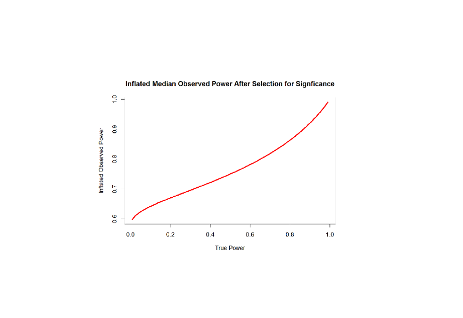
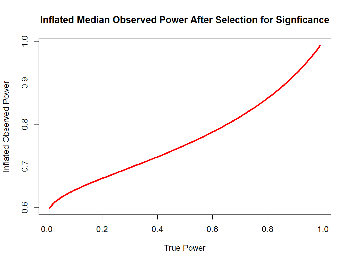
And here is a pretty picture of the relationship between true power and inflated observed power.  As we can see, there is more inflation for low true power because observed power after selection for significance has to be greater than 50%.  With alpha = .05 (two-tailed), when the null-hypothesis is true, inflated observed power is 61%.   Thus, an observed median power of 61% for only significant results supports the null-hypothesis.  With true power of 50%, observed power is inflated to 75%.  For high true power, the inflation is relatively small. With the recommended true power of 80%, median observed power for only significant results is 86%.

Observed power is easy to calculate from reported test statistics. The first step is to compute the exact two-tailed p-value.  These p-values can then be converted into observed power estimates using the standard normal distribution.

z.crit = qnorm(.975)
Obs.power = pnorm(qnorm(1-p/2),z.crit)

If there is selection for significance, you can use the previous formula to convert this observed power estimate into an estimate of true power.

This method assumes that (a) significant results are representative of the distribution and there are no additional biases (no p-hacking) and (b) all studies have the same or similar power.  This method does not work for heterogeneous sets of studies.

P.S.  It is possible to proof the formula that transforms true power into median observed power.  Another way to verify that the formula is correct is to confirm the predicted values with a simulation study.

Here is the code to run the simulation study:

n.sim = 100000
z.crit = qnorm(.975)
true.power = seq(.01,.99,.01)
obs.pow.sim = c()
for (i in 1:length(true.power)) {
z.sim = rnorm(n.sim,qnorm(true.power[i],z.crit))
med.z.sig = median(z.sim[z.sim > z.crit])
obs.pow.sim = c(obs.pow.sim,pnorm(med.z.sig,z.crit))
}
obs.pow.sim

obs.pow = pnorm(qnorm(true.power/2+(1-true.power),qnorm(true.power,z.crit)),z.crit)
obs.pow
cbind(true.power,obs.pow.sim,obs.pow)
plot(obs.pow.sim,obs.pow)