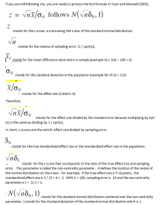
Yuan, K.-H., & Maxwell, S. (2005). On the Post Hoc Power in Testing Mean Differences. Journal of Educational and Behavioral Statistics, 141–167
This blog post provides an accessible introduction to the concept of observed power. Most of the statistical points are based on based on Yuan and Maxwell’s (2005 excellent but highly technical article about post-hoc power. This bog post tries to explain statistical concepts in more detail and uses simulation studies to illustrate important points.
What is Power?
Power is defined as the long-run probability of obtaining significant results in a series of exact replication studies. For example, 50% power means that a set of 100 studies is expected to produce 50 significant results and 50 non-significant results. The exact numbers in an actual set of studies will vary as a function of random sampling error, just like 100 coin flips are not always going to produce a 50:50 split of heads and tails. However, as the number of studies increases, the percentage of significant results will be ever closer to the power of a specific study.
A priori power
Power analysis can be useful for the planning of sample sizes before a study is being conducted. A power analysis that is being conducted before a study is called a priori power analysis (before = a priori). Power is a function of three parameters: the actual effect size, sampling error, and the criterion value that needs to be exceeded to claim statistical significance. In between-subject designs, sampling error is determined by sample size alone. In this special case, power is a function of the true effect size, the significance criterion and sample size.
The problem for researchers is that power depends on the effect size in the population (e.g., the true correlation between height and weight amongst Canadians in 2015). The population effect size is sometimes called the true effect size. Imagine that somebody would actually obtain data from everybody in a population. In this case, there is no sampling error and the correlation is the true correlation in the population. However, typically researchers use much smaller samples and the goal is to estimate the correlation in the population on the basis of a smaller sample. Unfortunately, power depends on the correlation in the population, which is unknown to a researcher planning a study. Therefore, researchers have to estimate the true effect size to compute an a priori power analysis.
Cohen (1988) developed general guidelines for the estimation of effect sizes. For example, in studies that compare the means of two groups, a standardized difference of half a standard deviation (e.g., 7.5 IQ points on an iQ scale with a standard deviation of 15) is considered a moderate effect. Researchers who assume that their predicted effect has a moderate effect size, can use d = .5 for an a priori power analysis. Assuming that they want to claim significance with the standard criterion of p < .05 (two-tailed), they would need N = 210 (n =105 per group) to have a 95% chance to obtain a significant result (GPower). I do not discuss a priori power analysis further because this blog post is about observed power. I merely introduced a priori power analysis to highlight the difference between a priori power analysis and a posteriori power analysis, which is the main topic of Yuan and Maxwell’s (2005) article.
A Posteriori Power Analysis: Observed Power
Observed power computes power after a study or several studies have been conducted. The key difference between a priori and a posteriori power analysis is that a posteriori power analysis uses the observed effect size in a study as an estimate of the population effect size. For example, assume a researcher found a correlation of r = .54 in a sample of N = 200 Canadians. Instead of guessing the effect size, the researcher uses the correlation observed in this sample as an estimate of the correlation in the population. There are several reasons why it might be interesting to conduct a power analysis after a study. First, the power analysis might be used to plan a follow up or replication study. Second, the power analysis might be used to examine whether a non-significant result might be the result of insufficient power. Third, observed power is used to examine whether a researcher used questionable research practices to produce significant results in studies that had insufficient power to produce significant results.
In sum, observed power is an estimate of the power of a study based on the observed effect size in a study. It is therefore not power that is being observed, but the effect size that is being observed. However, because the other parameters that are needed to compute power are known (sample size, significance criterion), the observed effect size is the only parameter that needs to be observed to estimate power. However, it is important to realize that observed power does not mean that power was actually observed. Observed power is still an estimate based on an observed effect size because power depends on the effect size in the population (which remains unobserved) and the observed effect size in a sample is just an estimate of the population effect size.
A Posteriori Power Analysis after a Single Study
Yuan and Maxwell (2005) examined the statistical properties of observed power. The main question was whether it is meaningful to compute observed power based on the observed effect size in a single study.
The first statistical analysis of an observed mean difference is to examine whether the study produced a significant result. For example, the study may have examined whether music lessons produce an increase in children’s IQ. The study had 95% power to produce a significant difference with N = 176 participants and a moderate effect size (d = .5; IQ = 7.5).
One possibility is that the study actually produced a significant result. For example, the observed IQ difference was 5 IQ points. This is less than the expected difference of 7.5 points and corresponds to a standardized effect size of d = .3. Yet, the t-test shows a highly significant difference between the two groups, t(208) = 3.6, p = 0.0004 (1 / 2513). The p-value shows that random sampling error alone would produce differences of this magnitude or more in only 1 out of 2513 studies. Importantly, the p-value only makes it very likely that the intervention contributed to the mean difference, but it does not provide information about the size of the effect. The true effect size may be closer to the expected effect size of 7.5 or it may be closer to 0. The true effect size remains unknown even after the mean difference between the two groups is observed. Yet, the study provides some useful information about the effect size. Whereas the a priori power analysis relied exclusively on guess-work, observed power uses the effect size that was observed in a reasonably large sample of 210 participants. Everything else being equal, effect size estimates based on 210 participants are more likely to match the true effect size than those based on 0 participants.
The observed effect size can be entered into a power analysis to compute observed power. In this example, observed power with an effect size of d = .3 and N = 210 (n = 105 per group) is 58%. One question examined by Yuan and Maxwell (2005) is whether it can be useful to compute observed power after a study produced a significant result.
The other question is whether it can be useful to compute observed power when a study produced a non-significant result. For example, assume that the estimate of d = 5 is overly optimistic and that the true effect size of music lessons on IQ is a more modest 1.5 IQ points (d = .10, one-tenth of a standard deviation). The actual mean difference that is observed after the study happens to match the true effect size exactly. The difference between the two groups is not statistically significant, t(208) = .72, p = .47. A non-significant result is difficult to interpret. On the one hand, the means trend in the right direction. On the other hand, the mean difference is not statistically significant. The p-value suggests that a mean difference of this magnitude would occur in every second study by chance alone even if music intervention had no effect on IQ at all (i.e., the true effect size is d = 0, the null-hypothesis is true). Statistically, the correct conclusion is that the study provided insufficient information regarding the influence of music lessons on IQ. In other words, assuming that the true effect size is closer to the observed effect size in a sample (d = .1) than to the effect size that was used to plan the study (d = .5), the sample size was insufficient to produce a statistically significant result. Computing observed power merely provides some quantitative information to reinforce this correct conclusion. An a posteriori power analysis with d = .1 and N = 210, yields an observed power of 11%. This suggests that the study had insufficient power to produce a significant result, if the effect size in the sample matches the true effect size.
Yuan and Maxwell (2005) discuss false interpretations of observed power. One false interpretation is that a significant result implies that a study had sufficient power. Power is a function of the true effect size and observed power relies on effect sizes in a sample. 50% of the time, effect sizes in a sample overestimate the true effect size and observed power is inflated. It is therefore possible that observed power is considerably higher than the actual power of a study.
Another false interpretation is that low power in a study with a non-significant result means that the hypothesis is correct, but that the study had insufficient power to demonstrate it. The problem with this interpretation is that there are two potential reasons for a non-significant result. One of them, is that a study had insufficient power to show a significant result when an effect is actually present (this is called the type-II error). The second possible explanation is that the null-hypothesis is actually true (there is no effect). A non-significant result cannot distinguish between these two explanations. Yet, it remains true that the study had insufficient power to test these hypotheses against each other. Even if a study had 95% power to show an effect if the true effect size is d = .5, it can have insufficient power if the true effect size is smaller. In the example, power decreased from 95% assuming d = .5, to 11% assuming d = .1.
Yuan and Maxell’s Demonstration of Systematic Bias in Observed Power
Yuan and Maxwell focus on a design in which a sample mean is compared against a population mean and the standard deviation is known. To modify the original example, a researcher could recruit a random sample of children, do a music lesson intervention and test the IQ after the intervention against the population mean of 100 with the population standard deviation of 15, rather than relying on the standard deviation in a sample as an estimate of the standard deviation. This scenario has some advantageous for mathematical treatments because it uses the standard normal distribution. However, all conclusions can be generalized to more complex designs. Thus, although Yuan and Maxwell focus on an unusual design, their conclusions hold for more typical designs such as the comparison of two groups that use sample variances (standard deviations) to estimate the variance in a population (i.e., pooling observed variances in both groups to estimate the population variance).
Yuan and Maxwell (2005) also focus on one-tailed tests, although the default criterion in actual studies is a two-tailed test. Once again, this is not a problem for their conclusions because the two-tailed criterion value for p = .05 is equivalent to the one-tailed criterion value for p = .025 (.05 / 2). For the standard normal distribution, the value is z = 1.96. This means that an observed z-score has to exceed a value of 1.96 to be considered significant.
To illustrate this with an example, assume that the IQ of 100 children after a music intervention is 103. After subtracting the population mean of 100 and dividing by the standard deviation of 15, the effect size is d = 3/15 = .2. Sampling error is defined by 1 / sqrt (n). With a sample size of n = 100, sampling error is .10. The test-statistic (z) is the ratio of the effect size and sampling error (.2 / .1) = 2. A z-score of 2 is just above the critical value of 2, and would produce a significant result, z = 2, p = .023 (one-tailed; remember criterion is .025 one-tailed to match .05 two-tailed). Based on this result, a researcher would be justified to reject the null-hypothesis (there is no effect of the intervention) and to claim support for the hypothesis that music lessons lead to an increase in IQ. Importantly, this hypothesis makes no claim about the true effect size. It merely states that the effect is greater than zero. The observed effect size in the sample (d = .2) provides an estimate of the actual effect size but the true effect size can be smaller or larger than the effect size in the sample. The significance test merely rejects the possibility that the effect size is 0 or less (i.e., music lessons lower IQ).
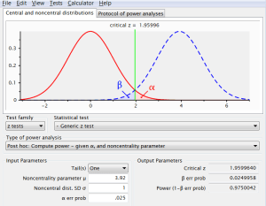
Entering a non-centrality parameter of 3 for a generic z-test in G*power yields the following illustration of a non-central distribution.

Illustration of non-central distribution using G*Power output
The red curve shows the standard normal distribution for the null-hypothesis. With d = 0, the non-centrality parameter is also 0 and the standard normal distribution is centered over zero.
The blue curve shows the non-central distribution. It is the same standard normal distribution, but now it is centered over z = 3. The distribution shows how z-scores would be distributed for a set of exact replication studies, where exact replication studies are defined as studies with the same true effect size and sampling error.
The figure also illustrates power by showing the critical z-score of 1.96 with a green line. On the left side are studies where sampling error reduced the observed effect size so much that the z-score was below 1.96 and produced a non-significant result (p > .025 one-tailed, p > .05, two-tailed). On the right side are studies with significant results. The area under the curve on the left side is called type-II error or beta-error). The area under the curve on the right side is called power (1 – type-II error). The output shows that beta error probability is 15% and Power is 85%.

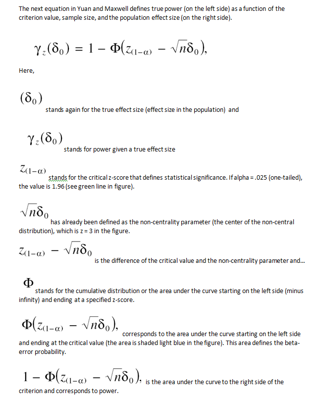
In sum, the formula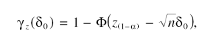
states that power for a given true effect size is the area under the curve to the right side of a critical z-score for a standard normal distribution that is centered over the non-centrality parameter that is defined by the ratio of the true effect size over sampling error.
[personal comment: I find it odd that sampling error is used on the right side of the formula but not on the left side of the formula. Power is a function of the non-centrality parameter and not just the effect size. Thus I would have included sqrt (n) also on the left side of the formula].
Because the formula relies on the true effect size, it specifies true power given the (unknown) population effect size. To use it for observed power, power has to be estimated based on the observed effect size in a sample.
The important novel contribution of Yuan and Maxwell (2005) was to develop a mathematical formula that relates observed power to true power and to find a mathematical formula for the bias in observed power.

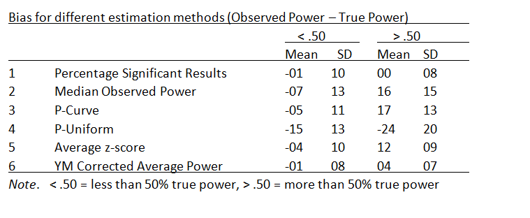
The formula implies that the amount of bias is a function of the unknown population effect size. Yuan and Maxwell make several additional observations about bias. First, bias is zero when true power is 50%. The second important observation is that systematic bias is never greater than 9 percentage points. The third observation is that power is overestimated when true power is less than 50% and underestimated when true power is above 50%. The last observation has important implications for the interpretation of observed power.
50% power implies that the test statistic matches the criterion value. For example, if the criterion is p < .05 (two-tailed), 50% power is equivalent to p = .05. If observed power is less than 50%, a study produced a non-significant result. A posteriori power analysis might suggest that observed power is only 40%. This finding suggests that the study was underpowered and that a more powerful study might produce a significant result. Systematic bias implies that the estimate of 40% is more likely to be an overestimation than an underestimation. As a result, bias does not undermine the conclusion. Rather observed power is conservative because the actual power is likely to be even less than 40%.
The alternative scenario is that observed power is greater than 50%, which implies a significant result. In this case, observed power might be used to argue that a study had sufficient power because it did produce a significant result. Observed power might show, however, that observed power is only 60%. This would indicate that there was a relatively high chance to end up with a non-significant result. However, systematic bias implies that observed power is more likely to underestimate true power than to overestimate it. Thus, true power is likely to be higher. Again, observed power is conservative when it comes to the interpretation of power for studies with significant results. This would suggest that systematic bias is not a serious problem for the use of observed power. Moreover, the systematic bias is never more than 9 percentage-points. Thus, observed power of 60% cannot be systematically inflated to more than 70%.
In sum, Yuan and Maxwell (2005) provided a valuable analysis of observed power and demonstrated analytically the properties of observed power.
Practical Implications of Yuan and Maxwell’s Findings
Based on their analyses, Yuan and Maxwell (2005) draw the following conclusions in the abstract of their article.
Using analytical, numerical, and Monte Carlo approaches, our results show that the estimated power does not provide useful information when the true power is small. It is almost always a biased estimator of the true power. The bias can be negative or positive. Large sample size alone does not guarantee the post hoc power to be a good estimator of the true power.
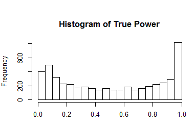
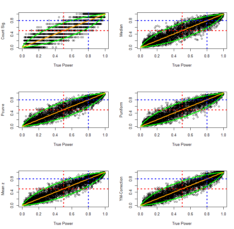
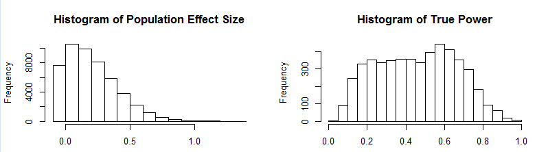
Unfortunately, other scientists often only read the abstract, especially when the article contains mathematical formulas that applied scientists find difficult to follow. As a result, Yuan and Maxwell’s (2005) article has been cited mostly as evidence that it observed power is a useless concept. I think this conclusion is justified based on Yuan and Maxwell’s abstract, but it does not follow from Yuan and Maxwell’s formula of bias. To make this point, I conducted a simulation study that paired 25 sample sizes (n = 10 to n = 250) and 20 effect sizes (d = .05 to d = 1) to create 500 non-centrality parameters. Observed effect sizes were randomly generated for a between-subject design with two groups (df = n*2 – 2). For each non-centrality parameter, two simulations were conducted for a total of 1000 studies with heterogeneous effect sizes and sample sizes (standard errors). The results are presented in a scatterplot with true power on the x-axis and observed power on the y-axis. The blue line shows prediction of observed power from true power. The red curve shows the biased prediction based on Yuan and Maxwell’s bias formula.
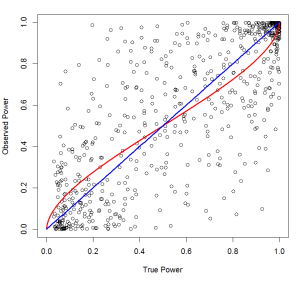
The most important observation is that observed power varies widely as a function of random sampling error in the observed effect sizes. In comparison, the systematic bias is relatively small. Moreover, observed power at the extremes clearly distinguishes between low powered (< 25%) and high powered (> 80%) power. Observed power is particularly informative when it is close to the maximum value of 100%. Thus, observed power of 99% or more strongly suggests that a study had high power. The main problem for posteriori power analysis is that observed effect sizes are imprecise estimates of the true effect size, especially in small samples. The next section examines the consequences of random sampling error in more detail.
Standard Deviation of Observed Power
Awareness has been increasing that point estimates of statistical parameters can be misleading. For example, an effect size of d = .8 suggests a strong effect, but if this effect size was observed in a small sample, the effect size is strongly influenced by sampling error. One solution to this problem is to compute a confidence interval around the observed effect size. The 95% confidence interval is defined by sampling error times 1.96; approximately 2. With sampling error of .4, the confidence interval could range all the way from 0 to 1.6. As a result, it would be misleading to claim that an effect size of d = .8 in a small sample suggests that the true effect size is strong. One solution to this problem is to report confidence intervals around point estimates of effect sizes. A common confidence interval is the 95% confidence interval. A 95% confidence interval means that there is a 95% probability that the population effect size is contained in the 95% confidence interval around the (biased) effect size in a sample.
To illustrate the use of confidence interval, I computed the confidence interval for the example of music training and IQ in children. The example assumes that the IQ of 100 children after a music intervention is 103. After subtracting the population mean of 100 and dividing by the standard deviation of 15, the effect size is d = 3/15 = .2. Sampling error is defined by 1 / sqrt (n). With a sample size of n = 100, sampling error is .10. To compute a 95% confidence interval, sampling error is multiplied with the z-scores that capture 95% of a standard normal distribution, which is 1.96. As sampling error is .10, the values are -.196 and .196. Given an observed effect size of d = .2, the 95% confidence interval ranges from .2 – .196 = .004 to .2 + .196 = .396.
A confidence interval can be used for significance testing by examining whether the confidence interval includes 0. If the 95% confidence interval does not include zero, it is possible to reject the hypothesis that the effect size in the population is 0, which is equivalent to rejecting the null-hypothesis. In the example, the confidence interval ends at d = .004, which implies that the null-hypothesis can be rejected. At the upper end, the confidence interval ends at d = .396. This implies that the empirical results also would reject hypotheses that the population effect size is moderate (d = .5) or strong (d = .8).
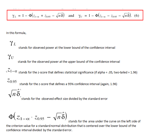
Confidence intervals around effect sizes are also useful for posteriori power analysis. Yuan and Maxwell (2005) demonstrated that confidence interval of observed power is defined by the observed power of the effect sizes that define the confidence interval of effect sizes.

The figure below illustrates the observed power for the lower bound of the confidence interval in the example of music lessons and IQ (d = .004).

The figure shows that the non-central distribution (blue) and the central distribution (red) nearly perfectly overlap. The reason is that the observed effect size (d = .004) is just slightly above the d-value of the central distribution when the effect size is zero (d = .000). When the null-hypothesis is true, power equals the type-I error rate (2.5%) because 2.5% of studies will produce a significant result by chance alone and chance is the only factor that produces significant results. When the true effect size is d = .004, power increases to 2.74 percent.
Remember that this power estimate is based on the lower limit of a 95% confidence interval around the observed power estimate of 50%. Thus, this result means that there is a 95% probability that the true power of the study is 2.5% when observed power is 50%.
The next figure illustrates power for the upper limit of the 95% confidence interval.
In this case, the non-central distribution and the central distribution overlap very little. Only 2.5% of the non-central distribution is on the left side of the criterion value, and power is 97.5%. This finding means that there is a 95% probability that true power is not greater than 97.5% when observed power is 50%.
Taken these results together, the results show that the 95% confidence interval around an observed power estimate of 50% ranges from 2.5% to 97.5%. As this interval covers pretty much the full range of possible values, it follows that observed power of 50% in a single study provides virtually no information about the true power of a study. True power can be anywhere between 2.5% and 97.5% percent.
The next figure illustrates confidence intervals for different levels of power.

The data are based on the same simulation as in the previous simulation study. The green line is based on computation of observed power for the d-values that correspond to the 95% confidence interval around the observed (simulated) d-values.
The figure shows that confidence intervals for most observed power values are very wide. The only accurate estimate of observed power can be achieved when power is high (upper right corner). But even 80% true power still has a wide confidence interval where the lower bound is below 20% observed power. Firm conclusions can only be drawn when observed power is high.
For example, when observed power is 95%, a one-sided 95% confidence interval (guarding only against underestimation) has a lower bound of 50% power. This finding would imply that observing power of 95% justifies the conclusion that the study had at least 50% power with an error rate of 5% (i.e., in 5% of the studies the true power is less than 50%).
The implication is that observed power is useless unless observed power is 95% or higher.
In conclusion, consideration of the effect of random sampling error on effect size estimates provides justification for Yuan and Maxwell’s (2005) conclusion that computation of observed power provides relatively little value. However, the reason is not that observed power is a problematic concept. The reason is that observed effect sizes in underpowered studies provide insufficient information to estimate observed power with any useful degree of accuracy. The same holds for the reporting of observed effect sizes that are routinely reported in research reports and for point estimates of effect sizes that are interpreted as evidence for small, moderate, or large effects. None of these statements are warranted when the confidence interval around these point estimates is taken into account. A study with d = .80 and a confidence interval of d = .01 to 1.59 does not justify the conclusion that a manipulation had a strong effect because the observed effect size is largely influenced by sampling error.
In conclusion, studies with large sampling error (small sample sizes) are at best able to determine the sign of a relationship. Significant positive effects are likely to be positive and significant negative effects are likely to be negative. However, the effect sizes in these studies are too strongly influenced by sampling error to provide information about the population effect size and therewith about parameters that depend on accurate estimation of population effect sizes like power.
Meta-Analysis of Observed Power
One solution to the problem of insufficient information in a single underpowered study is to combine the results of several underpowered studies in a meta-analysis. A meta-analysis reduces sampling error because sampling error creates random variation in effect size estimates across studies and aggregation reduces the influence of random factors. If a meta-analysis of effect sizes can produce more accurate estimates of the population effect size, it would make sense that meta-analysis can also increase the accuracy of observed power estimation.
Yuan and Maxwell (2005) discuss meta-analysis of observed power only briefly.
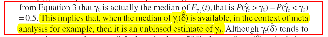
A problem in a meta-analysis of observed power is that observed power is not only subject to random sampling error, but also systematically biased. As a result, the average of observed power across a set of studies would also be systematically biased. However, the reason for the systematic bias is the non-symmetrical distribution of observed power when power is not 50%. To avoid this systematic bias, it is possible to compute the median. The median is unbiased because 50% of the non-central distribution is on the left side of the non-centrality parameter and 50% is on the right side of the non-centrality parameter. Thus, the median provides an unbiased estimate of the non-centrality parameter and the estimate becomes increasingly accurate as the number of studies in a meta-analysis increases.
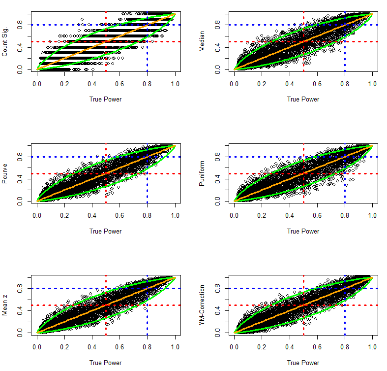
The next figure shows the results of a simulation with the same 500 studies (25 sample sizes and 20 effect sizes) that were simulated earlier, but this time each study was simulated to be replicated 1,000 times and observed power was estimated by computing the average or the median power across the 1,000 exact replication studies.

Purple = average observed power; Orange = median observed power
The simulation shows that Yuan and Maxwell’s (2005) bias formula predicts the relationship between true power and the average of observed power. It also confirms that the median is an unbiased estimator of true power and that observed power is a good estimate of true power when the median is based on a large set of studies. However, the question remains whether observed power can estimate true power when the number of studies is smaller.
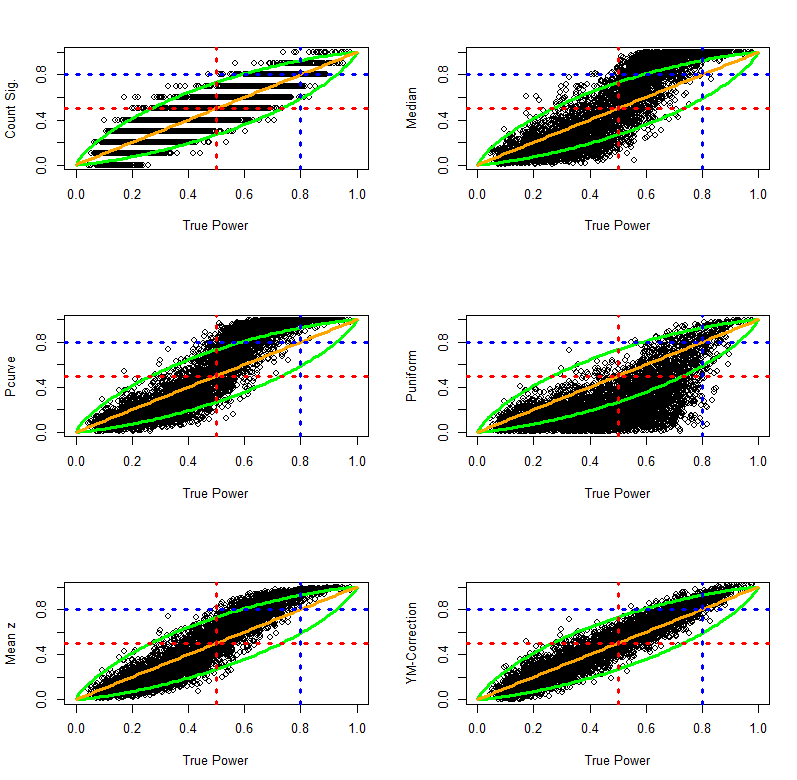
The next figure shows the results for a simulation where estimated power is based on the median observed power in 50 studies. The maximum discrepancy in this simulation was 15 percentage points. This is clearly sufficient to distinguish low powered studies (<50% power) from high powered studies (>80%).

To obtain confidence intervals for median observed power estimates, the power estimate can be converted into the corresponding non-centrality parameter of a standard normal distribution. The 95% confidence interval is defined as the standard deviation divided by the square root of the number of studies. The standard deviation of a standard normal distribution equals 1. Hence, the 95% confidence interval for a set of studies is defined by
Lower Limit = Normal (InverseNormal (power) – 1.96 / sqrt(k))
Upper Limit = Normal (inverseNormal(power) + 1.96 / sqrt(k))
Interestingly, the number of observations in a study is irrelevant. The reason is that larger samples produce smaller confidence intervals around an effect size estimate and increase power at the same time. To hold power constant, the effect size has to decrease and power decreases exponentially as effect sizes decrease. As a result, observed power estimates do not become more precise when sample sizes increase and effect sizes decrease proportionally.
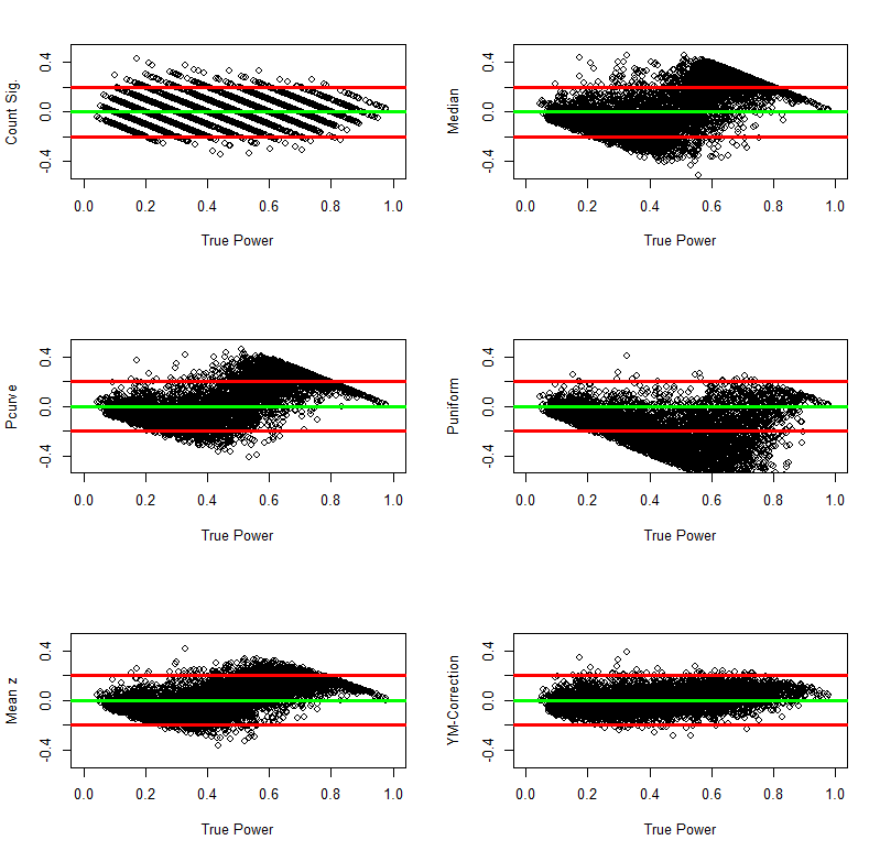
The next figure shows simulated data for 1000 studies with 20 effect sizes (0.05 to 1) and 25 sample sizes (n = 10 to 250). Each study was repeated 50 times and the median value was used to estimate true power. The green lines are the 95% confidence interval around the true power value. In real data, the confidence interval would be drawn around observed power, but observed power does not provide a clear mathematical function. The 95% confidence interval around the true power values is still useful because it predicts how much observed power estimates can deviate from true power. 95% of observed power values are expected to be within the area that is defined by lower and upper bound of the confidence interval. The Figure shows that most values are within the area. This confirms that sampling error in a meta-analysis of observed power is a function of the number of studies. The figure also shows that sampling error is greatest when power is 50%. In the tails of the distribution range restriction produces more precise estimates more quickly.

With 50 studies, the maximum absolute discrepancy is 15 percentage points. This level of precision is sufficient to draw broad conclusions about the power of a set of studies. For example, any median observed power estimate below 65% is sufficient to reveal that a set of studies had less power than Cohen’s recommended level of 80% power. A value of 35% would strongly suggest that a set of studies was severely underpowered.
Conclusion
Yuan and Maxwell (2005) provided a detailed statistical examination of observed power. They concluded that observed power typically provides little to no useful information about the true power of a single study. The main reason for this conclusion was that sampling error in studies with low power is too large to estimate true power with sufficient precision. The only precise estimate of power can be obtained when sampling error is small and effect sizes are large. In this case, power is near the maximum value of 1 and observed power correctly estimates true power as being close to 1. Thus, observed power can be useful when it suggests that a study had high power.
Yuan and Maxwell’s (2005) also showed that observed power is systematically biased unless true power is 50%. The amount of bias is relatively small and even without this systematic bias, the amount of random error is so large that observed power estimates based on a single study cannot be trusted.
Unfortunately, Yuan and Maxwell’s (2005) article has been misinterpreted as evidence that observed power calculations are inherently biased and useless. However, observed power can provide useful and unbiased information in a meta-analysis of several studies. First, a meta-analysis can provide unbiased estimates of power because the median value is an unbiased estimator of power. Second, aggregation across studies reduces random sampling error, just like aggregation across studies reduces sampling error in meta-analyses of effect sizes.
Implications
The demonstration that median observed power provides useful information about true power is important because observed power has become a valuable tool in the detection of publication bias and other biases that lead to inflated estimates of effect sizes. Starting with Sterling, Rosenbaum, and Weinkam ‘s(1995) seminal article, observed power has been used by Ioannidis and Trikalinos (2007), Schimmack (2012), Francis (2012), Simonsohn (2014), and van Assen, van Aert, and Wicherts (2014) to draw inferences about a set of studies with the help of posteriori power analysis. The methods differ in the way observed data are used to estimate power, but they all rely on the assumption that observed data provide useful information about the true power of a set of studies. This blog post shows that Yuan and Maxwell’s (2005) critical examination of observed power does not undermine the validity of statistical approaches that rely on observed data to estimate power.
Future Directions
This blog post focussed on meta-analysis of exact replication studies that have the same population effect size and the same sample size (sampling error). It also assumed that the set of studies is a representative set of studies. An important challenge for future research is to examine the statistical properties of observed power when power varies across studies (heterogeneity) and when publication bias and other biases are present. A major limitation of existing methods is that these methods assume a fixed population effect size (Ioannidis and Trikalinos (2007), Francis (2012), Simonsohn (2014), and van Assen, van Aert, and Wicherts (2014). At present, the Incredibility index (Schimmack, 2012) and the R-Index (Schimmack, 2014) have been proposed as methods for sets of studies that are biased and heterogeneous. An important goal for future research is to evaluate these methods in simulation studies with heterogeneous and biased sets of data.


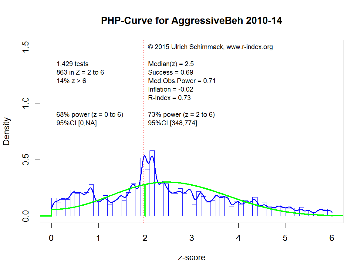
 The histogram and the blue density distribution show the observed data. The green curve shows the predicted distribution based on the post-hoc power analysis. Post-hoc power analysis suggests that the average power of significant results is 67%. Power for all statistical tests is estimated to be 58% (including 11% of z-scores greater than 6, power is .58*.89 + .11 = 63%). More important is the predicted distribution of z-scores. The predicted distribution on the left side of the criterion value matches the observed distribution rather well. This shows that there are not a lot of missing non-significant results. In other words, there does not appear to be a file-drawer of studies with non-significant results. There is also only a very small blip in the observed data just at the level of statistical significance. The close match between the observed and predicted distributions suggests that results in this journal are relatively free of systematic bias due to publication bias or questionable research practices.