Tag Archives: Statistics

Replacing p-values with Bayes-Factors: A Miracle Cure for the Replicability Crisis in Psychological Science

April 30, 2015UncategorizedBayes-Factors, Bayesian Statistics, Bem, Effect Size, ESP, Extrasensory Perception, http://dx.doi.org/10.1037/a0022790, http://pcl.missouri.edu/bayesfactor, Null-Hypothesis, p-values, Power, Replicability Crisis, Statistics, Type-I Error, Type-II Error, WagemakersUlrich Schimmack

How Science Should Work

Lay people, undergraduate students, and textbook authors have a simple model of science. Researchers develop theories that explain observable phenomena. These theories are based on exploratory research or deduced from existing theories. Based on a theory, researchers make novel predictions that can be subjected to empirical tests. The gold-standard for an empirical test is an experiment, but when experiments are impractical, quasi-experiments or correlational designs may be used. The minimal design examines whether two variables are related to each other. In an experiment, a relation exists when an experimentally created variation produces variation in observations on a variable of interest. In a correlational study, a relation exists when two variables covary with each other. When empirical results show the expected covariation, the results are considered supportive of a theory and the theory lives another day. When the expected covariation is not observed, the theory is challenged. If repeated attempts fail to show the expected effect, researchers start developing a new theory that is more consistent with the existing evidence. In this model of science, all scientists are only motivated by the goal to build a theory that is most consistent with a robust set of empirical findings.

The Challenge of Probabilistic Predictions and Findings

I distinguish two types of science; the distinction maps onto the distinction between hard and soft sciences, but I think the key difference between the two types of science is whether theories are used to test deterministic relationships (i.e., relationships that hold in virtually every test of the phenomenon) and probabilistic relationships, where a phenomenon may be observed only some of the time. An example of deterministic science is chemistry where the combination of oxygen and hydrogen leads to an explosion and water, when hydrogen and oxygen atoms combine to form H₂0. An example, of probabilistic science is a classic memory experiment where more recent information is more likely to be remembered than more remote information, but memory is not deterministic and it is possible that remote information is sometimes remembered better than recent information. A unique challenge for probabilistic science is to interpret empirical evidence because it is possible to make two errors in the interpretation of empirical results. These errors are called type-I and type-II errors.

Type-I errors refer to the error that the data show a theoretically predicted result when the prediction is false.

Type-II errors refer to the error that the data do not show a theoretically predicted result when the prediction is correct.

There are many reasons why a particular study may produce misleading results. Most prominently, a study may have failed to control (experimentally or statistically) for confounding factors. Another reason could be that a manipulation failed or a measure failed to measure the intended construct. Aside from these practical problems in conducting an empirical study, type-I and type-II errors can still emerge even in the most carefully conducted study with perfect measures. The reason is that empirical results in tests of probabilistic hypothesis are influenced by factors that are not under the control of the experimenter. These causal factors are sometimes called random error, sampling error, or random sampling error. The main purpose of inferential statistics is to deal with type-I and type-II errors that are caused by random error. It is also possible to conduct statistical analysis without drawing conclusions from the results. These statistics are often called descriptive statistics. For example, it is possible to compute and report the mean and standard deviation of a measure, the mean difference between two groups, or the correlation between two variables in a sample. As long as these results are merely reported they simply describe an empirical fact. They also do not test a theoretical hypothesis because scientific theories cannot make predictions about empirical results in a specific sample. Type-I or Type-II errors occur when the empirical results are used to draw inferences about results in future studies, in the population, or about the truth of theoretical predictions.

Three Approaches to the Problem of Probabilistic Science

In the world of probabilities, there is no certainty, but there are different degrees of uncertainty. As the strength of empirical evidence increases, it becomes less likely that researchers make type-I or type-II errors. The main aim of inferential statistics is to provide objective and quantitative information about the probability that empirical data provide the correct information about the hypothesis; that is to avoid making a type-I or type-II error.

Statisticians have developed three schools of thought: Fisherian, Neyman-Pearson, and Bayesian statistics. The problem is that contemporary proponents of these approaches are still fighting about the right approach. As a prominent statistician noted, “the effect on statistics of having three (actually more) warring factions… has not been good for our professional image” (Berger, 2003, p. 4). He goes on to note that statisticians have failed to make “a concerted professional effort to provide the scientific world with a unified testing methodology.”

For applied statisticians the distinction between Fisher and Neyman-Pearson is of relatively little practical concern because both approaches rely on the null-hypothesis and p-values. Statistics textbook often do present a hybrid model of both approaches. The Fisherian approach is to treat p-values as a measure of the strength of evidence against the null-hypothesis. As p-values approach zero, it becomes less and less likely that the null-hypothesis is true. For example, imagine a researcher computes the correlation between height and weight in a sample of N = 10 participants. The correlation is r = .50. Given the small sample size, this extreme deviation from the null-hypothesis could still have occurred by chance. As the sample size increases, random factors can produce only smaller and smaller deviations from zero and an observed correlation of r = .50 becomes less and less likely to have occurred as a result of random sampling error (oversampling tall and heavy participants and undersampling short and lightweight).

The main problem for Fisher’s approach is that it provides no guidelines about the size of a p-value that should be used to reject the null-hypothesis (there is no correlation) and therewith confirm the alternative (there is a correlation). Thus, p-values provide a quantitative measure of evidence against the null-hypothesis, but they do not provide a decision rule how strong the evidence should be to conclude that the null-hypothesis is false. As such, one might argue that Fisher’s approach is not an inferential statistical approach because it does not spell out how researchers should interpret p-values. Without a decision rule, a p-value is just an objective statistic like a sample mean or standard deviation.

Neyman-Pearson solved the problem of inference by introducing a criterion value. The most common criterion value is p = .05. When the strength of the evidence against the null-hypothesis leads to a p-value less than .05, the null-hypothesis is rejected. When the p-value is above the criterion, the null-hypothesis is accepted. According to Berger (2003), Neyman-Pearson also advocated to compute and report type-I and type-II error probabilities. Evidently, this suggestion has not been adopted in applied research, especially with regard to type-II error probabilities. The main reason for not adopting Neyman-Pearson’s recommendation is that the type-II error rate depends on an a priori assumption about the size of an effect. However, many hypothesis in the probabilities sciences make only diffuse, qualitative predictions (e.g., height will be positively correlated with weight, but the correlation may range anywhere from r = .1 to .8). Applied researchers saw little value in computing type-II error rates that are based on subjective assumptions about the strength of an effect. Instead, they adopted the criterion approach by Neyman-Pearson, but they used the criterion only to make the decision that the null-hypothesis is false when the evidence was strong enough to reject the null-hypothesis (p < .05). In contrast, when the evidence was not strong enough to reject the null-hypothesis, the results were considered inconclusive. The null-hypothesis could be true or the results were a type-II error. It was not important to determine whether the null-hypothesis was true or not because researchers were mainly interested in demonstrating causal relationships (a drug is effective) than in showing that something does not have an effect (a drug is not effective). By avoiding to rule in favor of the null-hypothesis, researchers could never make a type-II error in the classical sense that they falsely accepted the null-hypothesis. In this context, the term type-II error assumed a new meaning. A type-II error now meant that the study had insufficient statistical power to demonstrate that the null-hypothesis was false. A study with more statistical power might be able to produce a p-value less than .05 and demonstrate that the null-hypothesis is false.

The appeal of the hybrid approach was that the criterion provided meaningful information about the type-I error and that the type-II error rate was zero because results were never interpreted as favoring the null-hypothesis. The problem of this approach is that it can never lead to the conclusion that an effect is not present. For example, it is only possible to demonstrate gender differences, but it is never possible to demonstrate that men and women do not differ from each other. The main problem with this one-sided testing approach was that non-significant results seemed unimportant because they were inconclusive and it seemed more important to report conclusive, significant results than inconclusive and insignificant results. However, if only significant results are reported, it is no longer clear how many of these significant results might be type-I errors (Sterling, 1959). If only significant results are reported, the literature will be biased and can contain an undetermined amount of type-I errors (false evidence for an effect when the null-hypothesis is true). However, this is not a problem of p-values. It is a problem of not reporting studies that failed to provide support for a hypothesis, which is needed to reveal type-I errors. As type-I errors would occur only at a rate of 1 out of 20, honest reporting of all studies would quickly reveal which significant results are type-I errors.

Bayesian Statistics

The Bayesian tradition is not a unified approach to statistical inference. The main common element of Bayesian statistics is to criticize p-values because they do not provide information about the probability that a hypothesis is true; p(H1|D). Bayesians argue that empirical scientists misinterpret p-values as estimates of the probability that a hypothesis is true, when they quantify merely the probability that the data could have been produced without an effect. The main aim of Bayesian statistics is to use the Bayes Theorem to obtain an estimate of p(H1|D) from the empirically observed data.

One piece of information is the probability of an empirical observed statistic when the null-hypothesis is true, p(D|H0). This probability is closely related to p-values. Whereas the Bayesian p(D|H0) is the probability of obtaining a particular test statistic (e.g., a z-score of 1.65), p-values quantify the probability of obtaining a test statistic greater (one-sided) than the observed test statistic (p[z > 1.65] = .05) [for the two-sided case, p[abs(z) = 1.96] = .05]

The problem for estimating the probability that the hypothesis is true given an empirical result depends on three more probabilities that are unrelated to the observed data, namely the probability that the hypothesis is true, P(H0), the probability that the alternative hypothesis is true, p(H1), and the probability that the data would have been observed if the alternative hypothesis is true, p(D|H1). One approach to the problem of three unknowns is to use prior knowledge or empirical data to estimate these parameters. However, the problem for many empirical studies is that there is very little reliable a priori information that can be used to estimate these parameters.

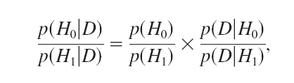
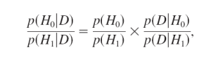
A group of Bayesian psychologists has advocated an objective Bayesian approach to deal with problem of unknown parameters in Bayes’ Theorem (Wagenmakers et al., 2011). To deal with the problem that p(H1|D) is unknown, the authors advocate using a default a priori probability distribution of effect sizes. The next step is to compute the ratio of p(H0|D) and p(H1|D). This ratio is called the Bayes-Factor. The following formula shows that the probability of the null-hypothesis being true given the data, p(H0|D), increases as the Bayes-Factor, p(D|H0)/p(D|H1) increases. Similarly, the probability of the alternative hypothesis given the data, p(H1|D) increases as the Bayes-Factor decreases. To quantify these probabilities, one would need to make assumptions about p(H0) and p(H1), but even without making assumptions about these probabilities, it is clear that the ratio of p(H0|D)/p(H1|D) is proportional to p(D|H0)/p(D|H1).

Bayes-Factors have two limitations. First, like p-values, Bayes-Factors alone are insufficient for inferential statistics because they only quantify the relative evidence in favor of two competing hypotheses. It is not clear at which point the results of a study should be interpreted as evidence for one of the two hypotheses. For example, is a Bayes-Factor of 1.1, 2.5, 3, 10, or 100 sufficient to conclude that the null-hypothesis is true? The second problem is that the default function may not adequately characterize the alternative hypothesis. In this regard, Bayesian statistics have the same problem as Neyman-Pearson’s approach that required making a priori assumptions about the effect size in order to compute type-II error rates. In Bayesian statistic the a priori distribution of effect sizes influences the Bayes-Factor.

In response to the first problem, Bayesians often use conventional criterion values that are used to make decisions based on empirical data. Commonly used criterion values are a Bayes-Factor of 3 or 10. A decision rule is clearly implemented in Bayesian studies with optional stopping where a Bayes-Factor of 10 or greater is used to justify terminating a study early. Bayes-Factors with a decision criterion create a new problem in that it is now possible to obtain inconclusive results and results that favor the null-hypothesis. As a result, there are now two types of type-II errors. Some type-II errors occur when the BF meets the criterion to accept the null-hypothesis when the null-hypothesis is false. Other type-II errors occur when the null-hypothesis is false and the data are inconclusive.

So far, Bayesian statisticians have not examined type-II error rates with the argument that Bayes-Factors do not require researchers to make decisions. However, without clear decision rules, Bayes-Factors are not very appealing to applied scientists because researchers, reviewers, editors, and readers need some rational criterion to make decisions about publication and planning of future studies. The best way to provide this information would be to examine how often Bayes-Factors of a certain magnitude lead to false conclusions; that is, to determine the type-I and type-II(a,b) error rates that are associated with a Bayes-Factor of a certain magnitude. This question has not been systematically examined.

The Bayesian Default T-Test

As noted above, there is no unified Bayesian approach to statistical inference. Thus, it is impossible to make general statements about Bayesian statistics. Here I focus on the statistical properties of the default Bayesian t-test (Rouder, Speckman, Sun, Morey, & Iverson, 2009). Most prominently, this test was used to demonstrate the superiority of Bayes-Factors over p-values with Bem’s (2011) controversial set of studies that seemed to support extrasensory perception.

The authors provide an R-package with a function that computes Bayes-Factors based on the observed t-statistic and degrees of freedom. It is noteworthy that the Bayes-Factor is fully determined by the t-value, the degrees of freedom, and a default scaling parameter for the prior distribution. As t-values and df are also used to compute p-values, Bayes-Factors and p-values are related to each other. The main difference is that p-values have a constant meaning for different sample sizes. That is, p = .04 has the same meaning in studies with N = 10, 100, or 1000 participants. However, Bayes-Factors for the same t-value changes as a function of sample size.

“With smaller sample sizes that are insufficient to differentiate between approximate and exact invariances, the Bayes factors allows researchers to gain evidence for the null. This evidence may be interpreted as support for at least an approximate invariance. In very large samples, however, the Bayes factor allows for the discovery of small perturbations that negate the existence of an exact invariance.” (Rouder et al., 2009, p 233).

This means that the same population effect size can produce three different outcomes depending on sample size; it may show evidence in favor of the null-hypothesis with a small sample size, it may show inconclusive results with a moderate sample size, and it may show evidence for the alternative hypothesis with a large sample size.

The ability to compute Bayes-Factors and p-values from t-values also implies that for a fixed sample size, p-values can be directly transformed into Bayes-Factors and vice versa. This makes it easy to directly compare the inferences that can be drawn from observed t-values for different p-values and Bayes-Factors.

The simulations used the default setting of a Cauchi distribution with a scale parameter of .707.

The x-axis shows potential effect sizes. The y-axis shows the weight attached to different effect sizes. The Cauchy distribution is centered over zero, giving the highest probability to an effect size of d = 0. As effect sizes increase weights decrease. However, even effect sizes greater than d = .8 (strong effect, Cohen, 1988) still have notable weights and the distribution includes effect sizes above d = 2. It is important to keep in mind that Bayes-Factors express the relative strength of evidence for or against the null-hypothesis relative to the weighted average effect size implied by the default function. Thus, it is possible that a Bayes-Factor favors the null-hypothesis if the population effect size is small because a small effect size is inconsistent with a prior distribution that considers strong effect sizes as a possible outcome.

The next figure shows Bayes-Factors as a function of p-values for an independent group t-test with n = 50 per condition. The black line shows the Bayes-Factor for H1 over H0. The red line shows the Bayes-Factor for H0 over H1. I show both ratios because I find it easier to compare Bayes-Factors greater than 1 than Bayes-Factors less than 1. The two lines cross when BF = 1, which is the point where the data favor both hypothesis equally.

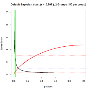
The graph shows the monotonic relationship between Bayes-Factors and p-values. As p-values decrease BF10 (favor H1 over H0, black) increases. As p-values increase, BF01-values (favor H0 over H1, red) also increase. However, the shapes of the two curves are rather different. As p-values decrease, the black line stays flat for a long time. As p-values are around p = .2, the curve goes up. It reaches a value of 3 just below a p-value of .05 (marked by the green line) and then increases quickly. This graph suggests that a Bayes-Factor of 3 corresponds roughly to a p-value of .05. A Bayes-Factor of 10 would correspond to a more stringent p-value. The red curve has a different shape. Starting from the left, it rises rather quickly and then slows down as p-values move towards 1. BF01 cross the red dotted line marking BF = 3 at around p = .3, but it never reaches a factor of 10 in favor of the null-hypothesis. Thus, using a criterion of BF = 3, p-values higher than .3 would be interpreted as evidence in favor of the null-hypothesis.

The next figure shows the same plot for different sample sizes.

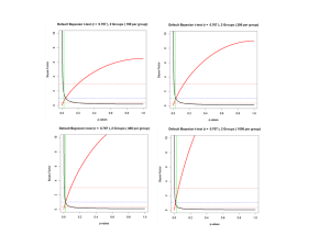
The graph shows how the Bayes-Factor of H0 over H1 (red line) increases as a function of sample size. It also reaches the critical value of BF = 3 earlier and earlier. With n = 1000 in each group (total N = 2000) the default Bayesian test is very likely to produce strong evidence in favor of either H1 or H0.

The responsiveness of BF01 to sample size makes sense. As sample size increases, statistical power to detect smaller and smaller effects also increases. In the limit a study with an infinite sample size has 100% power. That means, when the whole population has been studied and the effect size is zero, the null-hypothesis has been proven. However, even the smallest deviation from zero in the population will refute the null-hypothesis because sampling error is zero and the observed effect size is different from zero.

The graph also shows that Bayes-Factors and p-values provide approximately the same information when H1 is true. Statistical decisions based on BF10 or p-values lead to the same conclusion for matching criterion values. The standard criterion of p = .05 corresponds approximately to BF10 = 3 and BF10 = 10 corresponds roughly to p = .005. Thus, Bayes-Factors are not less likely to produce type-I errors than p-values because they reflect the same information, namely how unlikely it is that the deviation from zero in the sample is simply due to chance.

The main difference between Bayes-Factors and p-values arises in the interpretation of non-significant results (p > .05, BF10 < 3). The classic Neyman-Pearson approach would treat all non-significant results as evidence for the null-hypothesis, but would also try to quantify the type-II error rate (Berger, 2003). The Fisher-Neyman-Pearson hybrid approach treats all non-significant results as inconclusive and never decides in favor of the null-hypothesis. The default Bayesian t-tests distinguishes between inconclusive results and those that favor the null-hypothesis. To distinguish between these two conclusions, it is necessary to postulate a criterion value. Using the same criterion that is used to rule in favor of the alternative hypothesis (p = .05 ~ BF10 = 3), a BF01 > 3 is a reasonable criterion to decide in favor of the null-hypothesis. Moreover, a more stringent criterion would not be useful in small samples, because BF01 can never reach values of 10 or higher. Thus, in small samples, the conclusion would always be the same as in the standard approach that treats all non-significant results as inconclusive.

Power, Type I, and Type-II Error rates of the default Bayesian t-test with BF=3 as criterion value

As demonstrated in the previous section, the results of a default Bayesian t-test depend on the amount of sampling error, which is fully determined by sample size in a between-subject design. The previous results also showed that the default Bayesian t-test has modest power to rule in favor of the null-hypothesis in small samples.

For the first simulation, I used a sample size of n = 50 per group (N = 100). The reason is that Wagenmakers and colleagues have conducted several pre-registered replication studies with a stopping rule when sample size reaches N= 100. The simulation examines how often a default t-test with 100 participants can correctly identify the null-hypothesis when the null-hypothesis is true. The criterion value was set to BF01 = 3. As the previous graph showed, this implies that any observed p-value of approximately p = .30 to 1 is considered to be evidence in favor of the null-hypothesis. The simulation with 10,000 t-tests produced 6,927 BF01s greater than 3. This result is to be expected because p-values follow a uniform distribution when the null-hypothesis is true. Therefore, the p-value that corresponds to BF01 = 3 determines the rate of decisions in favor of null. With p = .30 as the criterion value that corresponds to BF01 = 3, 70% of the p-values are in the range from .30 to 1. 70% power may be deemed sufficient.

The next question is how the default Bayesian t-test behaves when the null-hypothesis is false. The answer to this question depends on the actual effect size. I conducted three simulation studies. The first simulation examined effect sizes in the moderate to large range (d = .5 to .8). Effect sizes were uniformly distributed. With a uniform distribution of effect sizes, true power ranges from 70% to 97% with an average power of 87% for the traditional criterion value of p = .05 (two-tailed). Consistent with this power analysis, the simulation produced 8704 significant results. Using the BF10 = 3 criterion, the simulation produced 7405 results that favored the alternative hypothesis with a Bayes-Factor greater than 3. The power is slightly lower than for p=.05 because BF = 3 is a slightly stricter criterion. More important, the power of the test to show support for the alternative is about equal to the power to support the null-hypothesis; 74% vs. 70%, respectively.

The next simulation examined effect sizes in the small to moderate range (d = .2 to .5). Power ranges from 17% to 70% with an average power of 42%. Consistent with this prediction, the simulation study with 10,000 t-tests produced 4072 significant results with p < .05 as criterion. With the somewhat stricter criterion of BF = 3, it produced only 2,434 results that favored the alternative hypothesis with BF > 3. More problematic is the finding that it favored the null-hypothesis (BF01 > 3) nearly as often, namely 2405 times. This means, that in a between-subject design with 100 participants and a criterion-value of BF = 3, the study has about 25% power to demonstrate that an effect is present, it will produce inconclusive results in 50% of all cases, and it will falsely support the null-hypothesis in 25% of all cases.

Things get even worse when the true effect size is very small (d > 0, d < .2). In this case, power ranges from just over .05, the type-I error rate, to just under 17% for d = .2. The average power is just 8%. Consistent with this prediction, the simulation produced only 823 out of 10,000 significant results with the traditional p = .05 criterion. The stricter BF = 3 criterion favored the alternative hypothesis in only 289 out of 10,000 cases with a BF greater than 3. However, BF01 exceeded a value of 3 in 6201 cases. The remaining 3519 cases produced inconclusive results. In this case, the Bayes-Factor favored the null-hypothesis when it was actually false. The rate of false decisions in favor of the null-hypothesis is nearly as high as the power of the test to correctly identify the null-hypothesis (62% vs. 70%).

The previous analyses indicate that Bayes-Factors produce meaningful results when power to detect an effect is high, but that Bayes-Factors are at risk to falsely favor the null-hypothesis when power is low. The next simulation directly examined the relationship between power and Bayes-Factors. The simulation used effect sizes in the range from d = .001 to d = 8 with N = 100. This creates a range of power from 5 to 97% with an average power of 51%.

In this figure, red data points show BF01 and blue data points show BF10. The right side of the figure shows that high-powered studies provide meaningful information about the population effect size as BF10 tend to be above the criterion value of 3 and BF01 are very rarely above the criterion value of 3. In contrast, on the left side, the results are misleading because most of the blue data points are below the criterion value of 3 and many BF01 data points are above the criterion value of BF = 3.

What about the probability of the data when the default alternative hypothesis is true?

A Bayes-Factor is defined as the ratio of two probabilities, the probability of the data when the null-hypothesis is true and the probability of the data when the null-hypothesis is false. As such, Bayes-Factors combine information about two hypotheses, but it might be informative to examine each hypothesis separately. What is the probability of the data when the null-hypothesis is true and what is the probability of the data when the alternative hypothesis is true? To examine this, I computed p(D|H1) by dividing the p-values by BF01 for t-values in the range from 0 to 5.

BF01 = p(D|H0) / p(D|H1) => p(D|H1) = BF01 * p(D|H0)

As Bayes-Factors are sensitive to sample size (degrees of freedom), I repeated the analysis with N = 40 (n = 20), N = 100 (n = 50), and N = 200 (n = 100).

The most noteworthy aspect of the figure is that p-values (the black line, p(D|H0)), are much more sensitive to changes in t-values than the probabilities of the data given the alternative hypothesis (yellow N=40, orange N=100, red N=200). The reason is the diffuse nature of the alternative hypothesis. It always includes a hypothesis that predicts the test-statistic, but it also includes many other hypotheses that make other predictions. This makes the relationship between the observed test-statistic, t, and the probability of t given the diffuse alternative hypothesis dull. The figure also shows that p(D|H0) and p(D|H1) both decrease monotonically as t-values increase. The reason is that the default prior distribution has its mode over 0. Thus, it also predicts that an effect size of 0 is the most likely outcome. It is therefore not a real alternative hypothesis that predicts an alternative effect size. It merely is a function that has a more muted relationship to the observed t-values. As a result, it is less compatible with low t-values and more compatible with high t-values than the steeper function for the point-null hypotheses.

Do we need Bayes-Factors to Provide Evidence in Favor of the Null-Hypothesis?

A common criticism of p-values is that they can only provide evidence against the null-hypothesis, but that they can never demonstrate that the null-hypothesis is true. Bayes-Factors have been advocated as a solution to this alleged problem. However, most researchers are not interested in testing the null-hypothesis. They want to demonstrate that a relationship exists. There are many reasons why a study may fail to produce the expected effect. However, when the predicted effect emerges, p-values can be used to rule out (with a fixed error probability) that the effect emerged simply as a result of chance alone.

Nevertheless, non-Bayesian statistics could also be used to examine whether a null-hypothesis is true without the need to construct diffuse priors or to compare the null-hypothesis to an alternative hypothesis. The approach is so simple that it is hard to find sources that explain it. Let’s assume that a researcher wants to test the null-hypothesis that Bayesian statisticians and other statisticians are equally intelligent. The researcher recruits 20 Bayesian statisticians and 20 frequentist statisticians and administers an IQ test. The Bayesian statisticians have an average IQ of 130 points. The frequentists have an average IQ of 120 points. The standard deviation of IQ scores on this IQ test is 15 points. Moreover, it has been shown that IQ scores are approximately normally distributed. Thus, sampling error is defined as 15 * (2 / sqrt(40)) = 4.7 ~ 5. The figure below shows the distribution of difference scores under the assumption that the null-hypothesis is true. The red lines show the 95% confidence interval. A 5 point difference is well within the 95% confidence interval. Thus, the result is consistent with the null-hypothesis that there is no difference in intelligence between the two groups. Of course, a 5 point difference is one-third of a standard deviation, but the sample size is simply too small to infer from the data that the null-hypothesis is false.

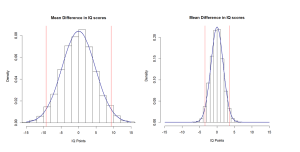
A more stringent test of the null-hypothesis would require a larger sample. A frequentist researcher conducts a power analysis and assumes that only a 5 point difference or more would be meaningful. She conducts a power analysis and finds that a study with 143 participants in each group (N = 286) is needed to have 80% power to show a difference of 5 points or more. A non-significant result would suggest that the difference is smaller or that a type-II error occurred with a 20% probability. The study yields a mean of 128 for frequentists and 125 for Bayesians. The 3 point difference is not significant. As a result, the data support the null-hypothesis that Bayesians and Frequentists do not differ in intelligence by more than 5 points. A more stringent test of equality or invariance would require an even larger sample. There is no magic Bayesian bullet that can test a precise null-hypothesis in small samples.

Ignoring Small Effects is Rational: Parsimony and Occam’s Razor

Another common criticism of p-values is that they are prejudice against the null-hypothesis because it is always possible to get a significant result simply by increasing sample size. With N = 1,000,000, a study has 95% power to detect even an effect size of d = .007. The argument is that it is meaningless to demonstrate significance in smaller samples, if it is certain that significance can always be obtained in a larger sample. The argument is flawed because it is simply not true that p-values will eventually produce a significant result when sample sizes increase. P-values will only produce significant results when a true effect exists. When the null-hypothesis is true an honest test of the hypothesis will only produce as many significant results as the type-I error criterion specifies. Moreover, Bayes-Factors are no solution to this problem. When a true effect exists, they will also favor the alternative hypothesis no matter how small the effect is and when sample sizes are large enough to have sufficient power. The only difference is that Bayes-Factors may falsely accept the null-hypothesis in smaller samples.

The more interesting argument against p-value is not that significant results in large studies are type-I errors, but that these results are practically meaningless. To make this point, statistics books often distinguish statistical significance and practical significance and warn that statistically significant results in large samples may have little practical significance. This warning was useful in the past when researchers would only report p-values (e.g., women have higher verbal intelligence than men, p < .05). The p-value says nothing about the size of the effect. When only the p-value is available, it makes sense to assume that significant results in smaller samples are larger because only large effects can be significant in these samples. However, large effects can also be significant in large samples and large effects in small studies can be inflated by sampling error. Thus, the notion of practical significance is outdated and should be replaced by questions about effect sizes. Neither p-values nor Bayes-Factors provide information about the size of the effect or the practical implications of a finding.

How can p-values be useful when there is clear evidence of a replication crisis?

Bem (2011) conducted 10 studies to demonstrate experimental evidence for anomalous retroactive influences on cognition and affect. His article reports 9 significant results and one marginally significant result. Subsequent studies have failed to replicate this finding. Wagenmakers et al. (2011) used Bem’s results as an example to highlight the advantages of Bayesian statistics. The logic was that p-values are flawed and that Bayes-Factors would have revealed that Bem’s (2011) evidence was weak. There are several problems with Wagenmaker et al.’s (2011) Bayesian analysis of Bem’s data.

First, the reported results differ from the default Bayesian-test implemented on Dr. Rouder’s website (http://pcl.missouri.edu/bf-one-sample). The reason is that Bayes-Factors depend on a scaling factor of the Cauchy distribution. Wagenmakers et al. (2011) used a scaling factor of 1, whereas the online app used .707 as the default. The choice of a scaling parameter gives some degrees of freedom to researchers. Researchers who favor the null-hypothesis can choose a larger scaling factor which makes the alternative hypothesis more extreme and easier to reject with small effects. Smaller scaling factors make the Cauchy-distribution narrower and it is easier to show evidence in favor of the alternative hypothesis with smaller effects. The behavior of Bayes-Factors for different scaling parameters is illustrated in Table 1 with Bem’s data.

Experiment 7 is highlighted because Bem (2011) already interpreted the non-significant result in this study as evidence that the effect disappears with supraliminal stimuli; that is, visible stimuli. The Bayes-Factor would support Bem’s (2011) conclusion that Experiment 7 shows evidence that the effect does not exist under this condition. The other studies essentially produced inconclusive Bayes-Factors, especially for the online default-setting with a scaling factor of .707. The only study that produced clear evidence for ESP was experiment 9. This study had the smallest sample size (N = 50), but a large effect size that was twice the effect size in the other studies. Of course, this difference is not reliable due to the small sample size, but it highlights how sensitive Bayes-Factors are to sampling error in small samples.

Another important feature of the Bayesian default t-test is that it centers the alternative hypothesis over 0. That is, it assigns the highest probability to the null-hypothesis, which is somewhat odd as the alternative hypothesis states that an effect should be present. The justification for this default setting is that the actual magnitude of the effect is unknown. However, it is typically possible to formulate an alternative hypothesis that allows for uncertainty, while predicting that the most likely outcome is a non-null effect size. This is especially true when previous studies provide some information about expected effect sizes. In fact, Bem (2011) explicitly planned his study with the expectation that the true effect size is small, d ~ .2. Moreover, it was demonstrated above that the default t-test is biased against small effects. Thus, the default Bayesian t-test with a scaling factor of 1 does not provide a fair test of Bem’s hypothesis against the null-hypothesis.

It is possible to use the default t-test to examine how consistent the data are with Bem’s (2011) a priori prediction that the effect size is d = .2. To do this, the null-hypothesis can be formulated as d = .2 and t-values can be computed as deviations from a population parameter d = .2. In this case, the null-hypothesis presents Bem’s (2011) a priori prediction and the alternative prediction is that observed effect sizes will deviated from this prediction because the effect is smaller (or larger). The next table shows the results for the Bayesian t-test that tests H0: d = .2 against a diffuse alternative H1: Cauchy-distribution centered over d = .2. Results are presented as BF01 so that Bayes-Factors greater than 3 indicate support for Bem’s (2011) prediction.

BF12

The Bayes-Factor supports Bem’s prediction in all tests. Choosing a wider alternative this time provides even stronger support for Bem’s prediction because the data are very consistent with the point prediction of a small effect size, d = .2. Moreover, even Experiment 7 now shows support for the hypothesis because an effect size of d = .09 is still more likely to have occurred when the effect size is d = .2 than for a wide-range of other effect sizes. Finally, Experiment 9 now shows the weakest support for the hypothesis. The reason is that Bem used only 50 participants in this study and the effect size was unusually large. This produced a low p-value in a test against zero, but it also produced the largest deviation from the a priori effect size of d = .2. However, this is to be expected in a small sample with large sampling error. Thus, the results are still supportive, but the evidence is rather weak compared to studies with larger samples and effect sizes close to d = 2.

The results demonstrate that Bayes-Factors cannot be interpreted as evidence for or against a specific hypothesis. They are influenced by the choice of the hypotheses that are being tested. In contrast, p-values have a consistent meaning. They quantify how probable it is that random sampling error alone could have produced a deviation between an observed sample parameter and a postulated population parameter. Bayesians have argued that this information is irrelevant and does not provide useful information for the testing of hypotheses. Although it is true that p-values do not quantify the probability that a hypothesis is true when significant results were observed, Bayes-Factors also do not provide this information. Moreover, Bayes-Factors are simply a ratio of two probabilities that compare two hypotheses against each other, but usually only one of the hypotheses is of theoretical interest. Without a principled and transparent approach to the formulation of alternative hypotheses, Bayes-Factors have no meaning and will change depending on different choices of the alternatives. The default approach aims to solve this by using a one-size-fits-all solution to the selection of priors. However, inappropriate priors will lead to invalid results and the diffuse Cauchy-distribution never fits any a priori theory.

Conclusion

Statisticians have been fighting for supremacy for decades. Like civilians in a war, empirical scientists have suffered from this war because they have been bombarded by propaganda and they have been criticized that they misunderstand statistics or use the wrong statistics. In reality, the statistical approaches are all related to each other and they all rely on the ratio of the observed effect sizes to sampling error (i.e, the signal to noise ratio) to draw inferences from observed data about hypotheses. Moreover, all statistical inferences are subject to the rule that studies with less sampling error provide more robust empirical evidence than studies with more sampling error. The biggest challenge for empirical researchers is to optimize the allocation of resources so that each study has high statistical power to produce a significant result when an effect exists. With high statistical power to detect an effect, p-values are likely to be small (50% chance to get a p-value of .005 or lower with 80% power) and Bayes-Factors and p-values provide virtually the same information for matching criterion values, when an effect is present. High power also implies a relative low frequency of type-II errors, which makes it more likely that a non-significant result occurred because the hypothesis is wrong. Thus, planning studies with high power is important no matter whether data are analyzed with Frequentist or Bayesian statistics.

Studies that aim to demonstrate the lack of an effect or an invariance (there is no difference in intelligence between Bayesian and frequentist statisticians) need large samples to demonstrate invariance or have to accept that there is a high probability that a larger study would find a reliable difference. Bayes-Factors do not provide a magical tool to provide strong support for the null-hypothesis in small samples. In small samples Bayes-Factors can falsely favor the null-hypothesis even when effect sizes are in the moderate to large range.

In conclusion, like p-values, Bayes-Factors are not wrong. They are mathematically defined entities. However, when p-values or Bayes-Factors are used by empirical scientists to interpret their data, it is important that the numeric results are interpreted properly. False interpretation of Bayes-Factors is just as problematic as false interpretation of p-values. Hopefully, this blog post provided some useful information about Bayes-Factors and their relationship to p-values.

An Introduction to Observed Power based on Yuan and Maxwell (2005)

March 24, 2015Introduction, Observed Power, Post-Hoc Power, Power, Statistics, Yuan and MaxwellBias, Median Observed Power, Meta-Analysis, Observed Power, Post-hoc Power, Power, Statistics, Yuan and MaxwellUlrich Schimmack

Yuan, K.-H., & Maxwell, S. (2005). On the Post Hoc Power in Testing Mean Differences. Journal of Educational and Behavioral Statistics, 141–167

This blog post provides an accessible introduction to the concept of observed power. Most of the statistical points are based on based on Yuan and Maxwell’s (2005 excellent but highly technical article about post-hoc power. This bog post tries to explain statistical concepts in more detail and uses simulation studies to illustrate important points.

What is Power?

Power is defined as the long-run probability of obtaining significant results in a series of exact replication studies. For example, 50% power means that a set of 100 studies is expected to produce 50 significant results and 50 non-significant results. The exact numbers in an actual set of studies will vary as a function of random sampling error, just like 100 coin flips are not always going to produce a 50:50 split of heads and tails. However, as the number of studies increases, the percentage of significant results will be ever closer to the power of a specific study.

A priori power

Power analysis can be useful for the planning of sample sizes before a study is being conducted. A power analysis that is being conducted before a study is called a priori power analysis (before = a priori). Power is a function of three parameters: the actual effect size, sampling error, and the criterion value that needs to be exceeded to claim statistical significance. In between-subject designs, sampling error is determined by sample size alone. In this special case, power is a function of the true effect size, the significance criterion and sample size.

The problem for researchers is that power depends on the effect size in the population (e.g., the true correlation between height and weight amongst Canadians in 2015). The population effect size is sometimes called the true effect size. Imagine that somebody would actually obtain data from everybody in a population. In this case, there is no sampling error and the correlation is the true correlation in the population. However, typically researchers use much smaller samples and the goal is to estimate the correlation in the population on the basis of a smaller sample. Unfortunately, power depends on the correlation in the population, which is unknown to a researcher planning a study. Therefore, researchers have to estimate the true effect size to compute an a priori power analysis.

Cohen (1988) developed general guidelines for the estimation of effect sizes. For example, in studies that compare the means of two groups, a standardized difference of half a standard deviation (e.g., 7.5 IQ points on an iQ scale with a standard deviation of 15) is considered a moderate effect. Researchers who assume that their predicted effect has a moderate effect size, can use d = .5 for an a priori power analysis. Assuming that they want to claim significance with the standard criterion of p < .05 (two-tailed), they would need N = 210 (n =105 per group) to have a 95% chance to obtain a significant result (GPower). I do not discuss a priori power analysis further because this blog post is about observed power. I merely introduced a priori power analysis to highlight the difference between a priori power analysis and a posteriori power analysis, which is the main topic of Yuan and Maxwell’s (2005) article.

A Posteriori Power Analysis: Observed Power

Observed power computes power after a study or several studies have been conducted. The key difference between a priori and a posteriori power analysis is that a posteriori power analysis uses the observed effect size in a study as an estimate of the population effect size. For example, assume a researcher found a correlation of r = .54 in a sample of N = 200 Canadians. Instead of guessing the effect size, the researcher uses the correlation observed in this sample as an estimate of the correlation in the population. There are several reasons why it might be interesting to conduct a power analysis after a study. First, the power analysis might be used to plan a follow up or replication study. Second, the power analysis might be used to examine whether a non-significant result might be the result of insufficient power. Third, observed power is used to examine whether a researcher used questionable research practices to produce significant results in studies that had insufficient power to produce significant results.

In sum, observed power is an estimate of the power of a study based on the observed effect size in a study. It is therefore not power that is being observed, but the effect size that is being observed. However, because the other parameters that are needed to compute power are known (sample size, significance criterion), the observed effect size is the only parameter that needs to be observed to estimate power. However, it is important to realize that observed power does not mean that power was actually observed. Observed power is still an estimate based on an observed effect size because power depends on the effect size in the population (which remains unobserved) and the observed effect size in a sample is just an estimate of the population effect size.

A Posteriori Power Analysis after a Single Study

Yuan and Maxwell (2005) examined the statistical properties of observed power. The main question was whether it is meaningful to compute observed power based on the observed effect size in a single study.

The first statistical analysis of an observed mean difference is to examine whether the study produced a significant result. For example, the study may have examined whether music lessons produce an increase in children’s IQ. The study had 95% power to produce a significant difference with N = 176 participants and a moderate effect size (d = .5; IQ = 7.5).

One possibility is that the study actually produced a significant result. For example, the observed IQ difference was 5 IQ points. This is less than the expected difference of 7.5 points and corresponds to a standardized effect size of d = .3. Yet, the t-test shows a highly significant difference between the two groups, t(208) = 3.6, p = 0.0004 (1 / 2513). The p-value shows that random sampling error alone would produce differences of this magnitude or more in only 1 out of 2513 studies. Importantly, the p-value only makes it very likely that the intervention contributed to the mean difference, but it does not provide information about the size of the effect. The true effect size may be closer to the expected effect size of 7.5 or it may be closer to 0. The true effect size remains unknown even after the mean difference between the two groups is observed. Yet, the study provides some useful information about the effect size. Whereas the a priori power analysis relied exclusively on guess-work, observed power uses the effect size that was observed in a reasonably large sample of 210 participants. Everything else being equal, effect size estimates based on 210 participants are more likely to match the true effect size than those based on 0 participants.

The observed effect size can be entered into a power analysis to compute observed power. In this example, observed power with an effect size of d = .3 and N = 210 (n = 105 per group) is 58%. One question examined by Yuan and Maxwell (2005) is whether it can be useful to compute observed power after a study produced a significant result.

The other question is whether it can be useful to compute observed power when a study produced a non-significant result. For example, assume that the estimate of d = 5 is overly optimistic and that the true effect size of music lessons on IQ is a more modest 1.5 IQ points (d = .10, one-tenth of a standard deviation). The actual mean difference that is observed after the study happens to match the true effect size exactly. The difference between the two groups is not statistically significant, t(208) = .72, p = .47. A non-significant result is difficult to interpret. On the one hand, the means trend in the right direction. On the other hand, the mean difference is not statistically significant. The p-value suggests that a mean difference of this magnitude would occur in every second study by chance alone even if music intervention had no effect on IQ at all (i.e., the true effect size is d = 0, the null-hypothesis is true). Statistically, the correct conclusion is that the study provided insufficient information regarding the influence of music lessons on IQ. In other words, assuming that the true effect size is closer to the observed effect size in a sample (d = .1) than to the effect size that was used to plan the study (d = .5), the sample size was insufficient to produce a statistically significant result. Computing observed power merely provides some quantitative information to reinforce this correct conclusion. An a posteriori power analysis with d = .1 and N = 210, yields an observed power of 11%. This suggests that the study had insufficient power to produce a significant result, if the effect size in the sample matches the true effect size.

Yuan and Maxwell (2005) discuss false interpretations of observed power. One false interpretation is that a significant result implies that a study had sufficient power. Power is a function of the true effect size and observed power relies on effect sizes in a sample. 50% of the time, effect sizes in a sample overestimate the true effect size and observed power is inflated. It is therefore possible that observed power is considerably higher than the actual power of a study.

Another false interpretation is that low power in a study with a non-significant result means that the hypothesis is correct, but that the study had insufficient power to demonstrate it. The problem with this interpretation is that there are two potential reasons for a non-significant result. One of them, is that a study had insufficient power to show a significant result when an effect is actually present (this is called the type-II error). The second possible explanation is that the null-hypothesis is actually true (there is no effect). A non-significant result cannot distinguish between these two explanations. Yet, it remains true that the study had insufficient power to test these hypotheses against each other. Even if a study had 95% power to show an effect if the true effect size is d = .5, it can have insufficient power if the true effect size is smaller. In the example, power decreased from 95% assuming d = .5, to 11% assuming d = .1.

Yuan and Maxell’s Demonstration of Systematic Bias in Observed Power

Yuan and Maxwell focus on a design in which a sample mean is compared against a population mean and the standard deviation is known. To modify the original example, a researcher could recruit a random sample of children, do a music lesson intervention and test the IQ after the intervention against the population mean of 100 with the population standard deviation of 15, rather than relying on the standard deviation in a sample as an estimate of the standard deviation. This scenario has some advantageous for mathematical treatments because it uses the standard normal distribution. However, all conclusions can be generalized to more complex designs. Thus, although Yuan and Maxwell focus on an unusual design, their conclusions hold for more typical designs such as the comparison of two groups that use sample variances (standard deviations) to estimate the variance in a population (i.e., pooling observed variances in both groups to estimate the population variance).

Yuan and Maxwell (2005) also focus on one-tailed tests, although the default criterion in actual studies is a two-tailed test. Once again, this is not a problem for their conclusions because the two-tailed criterion value for p = .05 is equivalent to the one-tailed criterion value for p = .025 (.05 / 2). For the standard normal distribution, the value is z = 1.96. This means that an observed z-score has to exceed a value of 1.96 to be considered significant.

To illustrate this with an example, assume that the IQ of 100 children after a music intervention is 103. After subtracting the population mean of 100 and dividing by the standard deviation of 15, the effect size is d = 3/15 = .2. Sampling error is defined by 1 / sqrt (n). With a sample size of n = 100, sampling error is .10. The test-statistic (z) is the ratio of the effect size and sampling error (.2 / .1) = 2. A z-score of 2 is just above the critical value of 2, and would produce a significant result, z = 2, p = .023 (one-tailed; remember criterion is .025 one-tailed to match .05 two-tailed). Based on this result, a researcher would be justified to reject the null-hypothesis (there is no effect of the intervention) and to claim support for the hypothesis that music lessons lead to an increase in IQ. Importantly, this hypothesis makes no claim about the true effect size. It merely states that the effect is greater than zero. The observed effect size in the sample (d = .2) provides an estimate of the actual effect size but the true effect size can be smaller or larger than the effect size in the sample. The significance test merely rejects the possibility that the effect size is 0 or less (i.e., music lessons lower IQ).

Entering a non-centrality parameter of 3 for a generic z-test in G*power yields the following illustration of a non-central distribution.

Illustration of non-central distribution using G*Power output

The red curve shows the standard normal distribution for the null-hypothesis. With d = 0, the non-centrality parameter is also 0 and the standard normal distribution is centered over zero.

The blue curve shows the non-central distribution. It is the same standard normal distribution, but now it is centered over z = 3. The distribution shows how z-scores would be distributed for a set of exact replication studies, where exact replication studies are defined as studies with the same true effect size and sampling error.

The figure also illustrates power by showing the critical z-score of 1.96 with a green line. On the left side are studies where sampling error reduced the observed effect size so much that the z-score was below 1.96 and produced a non-significant result (p > .025 one-tailed, p > .05, two-tailed). On the right side are studies with significant results. The area under the curve on the left side is called type-II error or beta-error). The area under the curve on the right side is called power (1 – type-II error). The output shows that beta error probability is 15% and Power is 85%.

In sum, the formula

states that power for a given true effect size is the area under the curve to the right side of a critical z-score for a standard normal distribution that is centered over the non-centrality parameter that is defined by the ratio of the true effect size over sampling error.

[personal comment: I find it odd that sampling error is used on the right side of the formula but not on the left side of the formula. Power is a function of the non-centrality parameter and not just the effect size. Thus I would have included sqrt (n) also on the left side of the formula].

Because the formula relies on the true effect size, it specifies true power given the (unknown) population effect size. To use it for observed power, power has to be estimated based on the observed effect size in a sample.

The important novel contribution of Yuan and Maxwell (2005) was to develop a mathematical formula that relates observed power to true power and to find a mathematical formula for the bias in observed power.

The formula implies that the amount of bias is a function of the unknown population effect size. Yuan and Maxwell make several additional observations about bias. First, bias is zero when true power is 50%. The second important observation is that systematic bias is never greater than 9 percentage points. The third observation is that power is overestimated when true power is less than 50% and underestimated when true power is above 50%. The last observation has important implications for the interpretation of observed power.

50% power implies that the test statistic matches the criterion value. For example, if the criterion is p < .05 (two-tailed), 50% power is equivalent to p = .05. If observed power is less than 50%, a study produced a non-significant result. A posteriori power analysis might suggest that observed power is only 40%. This finding suggests that the study was underpowered and that a more powerful study might produce a significant result. Systematic bias implies that the estimate of 40% is more likely to be an overestimation than an underestimation. As a result, bias does not undermine the conclusion. Rather observed power is conservative because the actual power is likely to be even less than 40%.

The alternative scenario is that observed power is greater than 50%, which implies a significant result. In this case, observed power might be used to argue that a study had sufficient power because it did produce a significant result. Observed power might show, however, that observed power is only 60%. This would indicate that there was a relatively high chance to end up with a non-significant result. However, systematic bias implies that observed power is more likely to underestimate true power than to overestimate it. Thus, true power is likely to be higher. Again, observed power is conservative when it comes to the interpretation of power for studies with significant results. This would suggest that systematic bias is not a serious problem for the use of observed power. Moreover, the systematic bias is never more than 9 percentage-points. Thus, observed power of 60% cannot be systematically inflated to more than 70%.

In sum, Yuan and Maxwell (2005) provided a valuable analysis of observed power and demonstrated analytically the properties of observed power.

Practical Implications of Yuan and Maxwell’s Findings

Based on their analyses, Yuan and Maxwell (2005) draw the following conclusions in the abstract of their article.

Using analytical, numerical, and Monte Carlo approaches, our results show that the estimated power does not provide useful information when the true power is small. It is almost always a biased estimator of the true power. The bias can be negative or positive. Large sample size alone does not guarantee the post hoc power to be a good estimator of the true power.

Unfortunately, other scientists often only read the abstract, especially when the article contains mathematical formulas that applied scientists find difficult to follow. As a result, Yuan and Maxwell’s (2005) article has been cited mostly as evidence that it observed power is a useless concept. I think this conclusion is justified based on Yuan and Maxwell’s abstract, but it does not follow from Yuan and Maxwell’s formula of bias. To make this point, I conducted a simulation study that paired 25 sample sizes (n = 10 to n = 250) and 20 effect sizes (d = .05 to d = 1) to create 500 non-centrality parameters. Observed effect sizes were randomly generated for a between-subject design with two groups (df = n*2 – 2). For each non-centrality parameter, two simulations were conducted for a total of 1000 studies with heterogeneous effect sizes and sample sizes (standard errors). The results are presented in a scatterplot with true power on the x-axis and observed power on the y-axis. The blue line shows prediction of observed power from true power. The red curve shows the biased prediction based on Yuan and Maxwell’s bias formula.

The most important observation is that observed power varies widely as a function of random sampling error in the observed effect sizes. In comparison, the systematic bias is relatively small. Moreover, observed power at the extremes clearly distinguishes between low powered (< 25%) and high powered (> 80%) power. Observed power is particularly informative when it is close to the maximum value of 100%. Thus, observed power of 99% or more strongly suggests that a study had high power. The main problem for posteriori power analysis is that observed effect sizes are imprecise estimates of the true effect size, especially in small samples. The next section examines the consequences of random sampling error in more detail.

Standard Deviation of Observed Power

Awareness has been increasing that point estimates of statistical parameters can be misleading. For example, an effect size of d = .8 suggests a strong effect, but if this effect size was observed in a small sample, the effect size is strongly influenced by sampling error. One solution to this problem is to compute a confidence interval around the observed effect size. The 95% confidence interval is defined by sampling error times 1.96; approximately 2. With sampling error of .4, the confidence interval could range all the way from 0 to 1.6. As a result, it would be misleading to claim that an effect size of d = .8 in a small sample suggests that the true effect size is strong. One solution to this problem is to report confidence intervals around point estimates of effect sizes. A common confidence interval is the 95% confidence interval. A 95% confidence interval means that there is a 95% probability that the population effect size is contained in the 95% confidence interval around the (biased) effect size in a sample.

To illustrate the use of confidence interval, I computed the confidence interval for the example of music training and IQ in children. The example assumes that the IQ of 100 children after a music intervention is 103. After subtracting the population mean of 100 and dividing by the standard deviation of 15, the effect size is d = 3/15 = .2. Sampling error is defined by 1 / sqrt (n). With a sample size of n = 100, sampling error is .10. To compute a 95% confidence interval, sampling error is multiplied with the z-scores that capture 95% of a standard normal distribution, which is 1.96. As sampling error is .10, the values are -.196 and .196. Given an observed effect size of d = .2, the 95% confidence interval ranges from .2 – .196 = .004 to .2 + .196 = .396.

A confidence interval can be used for significance testing by examining whether the confidence interval includes 0. If the 95% confidence interval does not include zero, it is possible to reject the hypothesis that the effect size in the population is 0, which is equivalent to rejecting the null-hypothesis. In the example, the confidence interval ends at d = .004, which implies that the null-hypothesis can be rejected. At the upper end, the confidence interval ends at d = .396. This implies that the empirical results also would reject hypotheses that the population effect size is moderate (d = .5) or strong (d = .8).

Confidence intervals around effect sizes are also useful for posteriori power analysis. Yuan and Maxwell (2005) demonstrated that confidence interval of observed power is defined by the observed power of the effect sizes that define the confidence interval of effect sizes.

The figure below illustrates the observed power for the lower bound of the confidence interval in the example of music lessons and IQ (d = .004).

The figure shows that the non-central distribution (blue) and the central distribution (red) nearly perfectly overlap. The reason is that the observed effect size (d = .004) is just slightly above the d-value of the central distribution when the effect size is zero (d = .000). When the null-hypothesis is true, power equals the type-I error rate (2.5%) because 2.5% of studies will produce a significant result by chance alone and chance is the only factor that produces significant results. When the true effect size is d = .004, power increases to 2.74 percent.

Remember that this power estimate is based on the lower limit of a 95% confidence interval around the observed power estimate of 50%. Thus, this result means that there is a 95% probability that the true power of the study is 2.5% when observed power is 50%.

The next figure illustrates power for the upper limit of the 95% confidence interval.

In this case, the non-central distribution and the central distribution overlap very little. Only 2.5% of the non-central distribution is on the left side of the criterion value, and power is 97.5%. This finding means that there is a 95% probability that true power is not greater than 97.5% when observed power is 50%.

Taken these results together, the results show that the 95% confidence interval around an observed power estimate of 50% ranges from 2.5% to 97.5%. As this interval covers pretty much the full range of possible values, it follows that observed power of 50% in a single study provides virtually no information about the true power of a study. True power can be anywhere between 2.5% and 97.5% percent.

The next figure illustrates confidence intervals for different levels of power.

The data are based on the same simulation as in the previous simulation study. The green line is based on computation of observed power for the d-values that correspond to the 95% confidence interval around the observed (simulated) d-values.

The figure shows that confidence intervals for most observed power values are very wide. The only accurate estimate of observed power can be achieved when power is high (upper right corner). But even 80% true power still has a wide confidence interval where the lower bound is below 20% observed power. Firm conclusions can only be drawn when observed power is high.

For example, when observed power is 95%, a one-sided 95% confidence interval (guarding only against underestimation) has a lower bound of 50% power. This finding would imply that observing power of 95% justifies the conclusion that the study had at least 50% power with an error rate of 5% (i.e., in 5% of the studies the true power is less than 50%).

The implication is that observed power is useless unless observed power is 95% or higher.

In conclusion, consideration of the effect of random sampling error on effect size estimates provides justification for Yuan and Maxwell’s (2005) conclusion that computation of observed power provides relatively little value. However, the reason is not that observed power is a problematic concept. The reason is that observed effect sizes in underpowered studies provide insufficient information to estimate observed power with any useful degree of accuracy. The same holds for the reporting of observed effect sizes that are routinely reported in research reports and for point estimates of effect sizes that are interpreted as evidence for small, moderate, or large effects. None of these statements are warranted when the confidence interval around these point estimates is taken into account. A study with d = .80 and a confidence interval of d = .01 to 1.59 does not justify the conclusion that a manipulation had a strong effect because the observed effect size is largely influenced by sampling error.

In conclusion, studies with large sampling error (small sample sizes) are at best able to determine the sign of a relationship. Significant positive effects are likely to be positive and significant negative effects are likely to be negative. However, the effect sizes in these studies are too strongly influenced by sampling error to provide information about the population effect size and therewith about parameters that depend on accurate estimation of population effect sizes like power.

Meta-Analysis of Observed Power

One solution to the problem of insufficient information in a single underpowered study is to combine the results of several underpowered studies in a meta-analysis. A meta-analysis reduces sampling error because sampling error creates random variation in effect size estimates across studies and aggregation reduces the influence of random factors. If a meta-analysis of effect sizes can produce more accurate estimates of the population effect size, it would make sense that meta-analysis can also increase the accuracy of observed power estimation.

Yuan and Maxwell (2005) discuss meta-analysis of observed power only briefly.

A problem in a meta-analysis of observed power is that observed power is not only subject to random sampling error, but also systematically biased. As a result, the average of observed power across a set of studies would also be systematically biased. However, the reason for the systematic bias is the non-symmetrical distribution of observed power when power is not 50%. To avoid this systematic bias, it is possible to compute the median. The median is unbiased because 50% of the non-central distribution is on the left side of the non-centrality parameter and 50% is on the right side of the non-centrality parameter. Thus, the median provides an unbiased estimate of the non-centrality parameter and the estimate becomes increasingly accurate as the number of studies in a meta-analysis increases.

The next figure shows the results of a simulation with the same 500 studies (25 sample sizes and 20 effect sizes) that were simulated earlier, but this time each study was simulated to be replicated 1,000 times and observed power was estimated by computing the average or the median power across the 1,000 exact replication studies.

Purple = average observed power; Orange = median observed power

The simulation shows that Yuan and Maxwell’s (2005) bias formula predicts the relationship between true power and the average of observed power. It also confirms that the median is an unbiased estimator of true power and that observed power is a good estimate of true power when the median is based on a large set of studies. However, the question remains whether observed power can estimate true power when the number of studies is smaller.

The next figure shows the results for a simulation where estimated power is based on the median observed power in 50 studies. The maximum discrepancy in this simulation was 15 percentage points. This is clearly sufficient to distinguish low powered studies (<50% power) from high powered studies (>80%).

To obtain confidence intervals for median observed power estimates, the power estimate can be converted into the corresponding non-centrality parameter of a standard normal distribution. The 95% confidence interval is defined as the standard deviation divided by the square root of the number of studies. The standard deviation of a standard normal distribution equals 1. Hence, the 95% confidence interval for a set of studies is defined by

Lower Limit = Normal (InverseNormal (power) – 1.96 / sqrt(k))

Upper Limit = Normal (inverseNormal(power) + 1.96 / sqrt(k))

Interestingly, the number of observations in a study is irrelevant. The reason is that larger samples produce smaller confidence intervals around an effect size estimate and increase power at the same time. To hold power constant, the effect size has to decrease and power decreases exponentially as effect sizes decrease. As a result, observed power estimates do not become more precise when sample sizes increase and effect sizes decrease proportionally.

The next figure shows simulated data for 1000 studies with 20 effect sizes (0.05 to 1) and 25 sample sizes (n = 10 to 250). Each study was repeated 50 times and the median value was used to estimate true power. The green lines are the 95% confidence interval around the true power value. In real data, the confidence interval would be drawn around observed power, but observed power does not provide a clear mathematical function. The 95% confidence interval around the true power values is still useful because it predicts how much observed power estimates can deviate from true power. 95% of observed power values are expected to be within the area that is defined by lower and upper bound of the confidence interval. The Figure shows that most values are within the area. This confirms that sampling error in a meta-analysis of observed power is a function of the number of studies. The figure also shows that sampling error is greatest when power is 50%. In the tails of the distribution range restriction produces more precise estimates more quickly.

With 50 studies, the maximum absolute discrepancy is 15 percentage points. This level of precision is sufficient to draw broad conclusions about the power of a set of studies. For example, any median observed power estimate below 65% is sufficient to reveal that a set of studies had less power than Cohen’s recommended level of 80% power. A value of 35% would strongly suggest that a set of studies was severely underpowered.

Conclusion

Yuan and Maxwell (2005) provided a detailed statistical examination of observed power. They concluded that observed power typically provides little to no useful information about the true power of a single study. The main reason for this conclusion was that sampling error in studies with low power is too large to estimate true power with sufficient precision. The only precise estimate of power can be obtained when sampling error is small and effect sizes are large. In this case, power is near the maximum value of 1 and observed power correctly estimates true power as being close to 1. Thus, observed power can be useful when it suggests that a study had high power.

Yuan and Maxwell’s (2005) also showed that observed power is systematically biased unless true power is 50%. The amount of bias is relatively small and even without this systematic bias, the amount of random error is so large that observed power estimates based on a single study cannot be trusted.

Unfortunately, Yuan and Maxwell’s (2005) article has been misinterpreted as evidence that observed power calculations are inherently biased and useless. However, observed power can provide useful and unbiased information in a meta-analysis of several studies. First, a meta-analysis can provide unbiased estimates of power because the median value is an unbiased estimator of power. Second, aggregation across studies reduces random sampling error, just like aggregation across studies reduces sampling error in meta-analyses of effect sizes.

Implications

The demonstration that median observed power provides useful information about true power is important because observed power has become a valuable tool in the detection of publication bias and other biases that lead to inflated estimates of effect sizes. Starting with Sterling, Rosenbaum, and Weinkam ‘s(1995) seminal article, observed power has been used by Ioannidis and Trikalinos (2007), Schimmack (2012), Francis (2012), Simonsohn (2014), and van Assen, van Aert, and Wicherts (2014) to draw inferences about a set of studies with the help of posteriori power analysis. The methods differ in the way observed data are used to estimate power, but they all rely on the assumption that observed data provide useful information about the true power of a set of studies. This blog post shows that Yuan and Maxwell’s (2005) critical examination of observed power does not undermine the validity of statistical approaches that rely on observed data to estimate power.

Future Directions

This blog post focussed on meta-analysis of exact replication studies that have the same population effect size and the same sample size (sampling error). It also assumed that the set of studies is a representative set of studies. An important challenge for future research is to examine the statistical properties of observed power when power varies across studies (heterogeneity) and when publication bias and other biases are present. A major limitation of existing methods is that these methods assume a fixed population effect size (Ioannidis and Trikalinos (2007), Francis (2012), Simonsohn (2014), and van Assen, van Aert, and Wicherts (2014). At present, the Incredibility index (Schimmack, 2012) and the R-Index (Schimmack, 2014) have been proposed as methods for sets of studies that are biased and heterogeneous. An important goal for future research is to evaluate these methods in simulation studies with heterogeneous and biased sets of data.

A Playful Way to Learn about Power, Publication Bias, and the R-Index: Simulate questionable research methods and see what happens.

December 31, 2014UncategorizedPower, Publicatin Bias, Questionable Reserach Practices, r-index, Simulation, StatisticsUlrich Schimmack

This blog introduces a simple excel spreadsheet that simulates the effect of excluding non-significant results from an unbiased set of studies.

The results in the most left column show the results for an unbiased set of 100 studies (N = 100, dropped = 0). The power value is used to compute the observed power in the 100 studies based on a normal distribution around the non-centrality parameter corresponding to the power value (e.g., power = .50, ncp = 1.96).

For an unbiased set of studies, median observed power is equivalent to the success rate (percentage of significant results) in a set of studies. For example, with 50% power, the median observed ncp is 1.96, which is equivalent to the true ncp of 1.96 that corresponds to 50% power. In this case, the success rate is 50%. As the success rate is equivalent to median observed power, there is no inflation in the success rate and the inflation rate is 0. As a result, the R-Index is equivalent to median observed power and success rate. R-Index = Median Observed Power – Inflation Rate; .50 = .50 – 0.

Moving to the right, studies with the lowest observed ncp values (equivalent to the highest p-values) are dropped in sets of 5 studies. However, you can make changes to the way results are excluded or altered to simulate questionable research practices. When non-significant studies are dropped, median observed power and success rate increase. Eventually, the success rate increases faster than median observed power, leading to a positive inflation rate. As the inflation rate is subtracted from median observed power, the R-Index starts to correct for publication bias. For example, in the example with 50% true power, median observed power is inflated to 63% by dropping 25 non-significant results. The success rate is 67%, the inflation rate is 4% and the R-Index is 59%. Thus, the R-Index still overestimates true power by 9%, but it provides a better estimate of true power than median observed power without a correction (63%).

An important special case is the scenario where all non-significant results are dropped. This scenario is automatically highlighted with orange cells for the number of studies and success rate. With 50% true power, the event occurs when 50% of the studies are dropped. In this scenario, median observed power is 76%, the success rate is 100%, inflation rate is 24% and the R-Index is 51%. These values are slightly different from more exact simulations which show 75% median observed power, 25% inflation rate and an R-Index of 50%.

The table below lists the results for different levels of true power when all non-significant results are dropped. The scenario with 5% power implies that the null-hypothesis is true, but that 5% of significant results are obtained due to sampling error alone.

True Power MOP IR R-Index

5%                     66           34           32
30%                     70           30           40
50%                     75           25           50
65%                     80           20           60
80%                     87           13           73
95%                     96           04           91
Success Rate is fixed at 100%; MOP = median observed power; IR = Inflation Rate, R-Index

The results show that the R-Index tracks observed power, but it is not an unbiased estimate of true power. In real data the process that leads to bias is unknown and it is impossible to obtain an unbiased estimate of true power from a biased set of studies. This is the reason why it is important to eliminate biases in publications as much as possible. However, the R-Index provides some useful information about the true power and replicability in a biased set of studies.

Simulation R-Index [click on link to download spreadsheet]

Roy Baumeister’s R-Index

December 1, 2014Baumeister, r-indexIncredibility Index, Questionable Research Practices, r-index, replicability, Roy Baumeister, StatisticsUlrich Schimmack

“We did run multiple studies, some of which did not work, and some of which worked better than others. You may think that not reporting the less successful studies is wrong, but that is how the field works.” (Roy Baumeister, personal email communication)

The R-Index can be used to evaluate the replicability of a set of statistical results. It can be used to evaluate the statistical research integrity of journals, articles on a specific topic (meta-analysis), and researchers. Just like the H-Index has become a popular metric of research excellence, the R-Index of individual researchers can be used to evaluate the replicability of their findings.

I chose Roy Baumeister as an example for several reasons. First, the R-Index is based on my earlier work on the incredibility-index (Schimmack, 2012). In this article, I demonstrated how power analysis can be used to reveal that researchers used questionable research practices to produce statistically significant results. I illustrated this approach with two articles. One article published 10 experiments that appeared to demonstrate time-reversed causality. Independent replication studies failed to replicate this incredible finding. The Incredibility-Index predicted this failure. The second article was a study on glucose consumption and will-power with Roy Baumeister as the senior author. The Incredibility-Index showed that the statistical results reported in this article were even less credible than the time-travel studies in Bem’s (2011) article.

Not surprisingly, Roy Baumeister was a reviewer of the incredibility article. During the review process, Roy Baumeister explained why his article reported more significant results than one would expect on the basis of the statistical power of these studies.

“My paper with Gailliot et al. (2007) is used as an illustration here. Of course, I am quite familiar with the process and history of that one. We initially submitted it with more studies, some of which had weaker results. The editor said to delete those. He wanted the paper shorter so as not to use up a lot of journal space with mediocre results. It worked: the resulting paper is shorter and stronger. Does that count as magic? The studies deleted at the editor’s request are not the only story. I am pretty sure there were other studies that did not work. Let us suppose that our hypotheses were correct and that our research was impeccable. Then several of our studies would have failed, simply given the realities of low power and random fluctuations. Is anyone surprised that those studies were not included in the draft we submitted for publication? If we had included them, certainly the editor and reviewers would have criticized them and formed a more negative impression of the paper. Let us suppose that they still thought the work deserved publication (after all, as I said, we are assuming here that the research was impeccable and the hypotheses correct). Do you think the editor would have wanted to include those studies in the published version?”

To my knowledge this is one of the few frank acknowledgements that questionable research practices (i.e., excluding evidence that does not support an author’s theory) contributed to the picture-perfect results in a published article. It is therefore instructive to examine the R-Index of a researcher who openly acknowledged that the reported results are a biased selection of the empirical evidence.

A tricky issue in any statistical analysis is the sampling of studies. In this case it would be possible to conduct the analysis on the full set of articles published by Roy Baumeister. However, for my analysis I selected a sample. To ensure that the sample is unbiased, I chose a sampling strategy that makes a priori sense and does not involve random sampling because I have control over the random generator. My sampling strategy was to focus on the Top 10 most cited original research articles.

To evaluate the R-Index, it is instructive to keep the following scenarios in mind.

The null-hypothesis is true and a researcher uses questionable research practices to obtain just significant results (p = .049999). The observed power for this set of studies is 50%, but all statistical results are significant, 100% success rate. The success rate is inflated by 50%. The R-Index is observed power minus inflation rate, which is 0%.
The null-hypothesis is true and a researcher drops non-significant results and/or uses questionable research methods that capitalize on chance. In this case, p-values above .05 are not reported and p-values below .05 have a uniform distribution with a median of .025. A p-value of .025 corresponds to 61% observed power. With 100% significant results, the inflation rate is 39%, and the R-Index is 22% (61%-39%).
The null-hypothesis is false and researcher conducts studies with 30% power. The non-significant studies are not published. In this case, observed power is 70%. With 100% success rate, the inflation rate is 30%. The R-Index is 40%.
The null-hypothesis is false and researcher conducts studies with 50% power. The non-significant studies are not published. In this case, observed power is 75%. With 100% success rate, the inflation rate is 25%. The R-Index is 50%.
The null-hypothesis is false and researchers conduct studies with 80% power, as recommended by Cohen. The non-significant results are not published (20% missing). In this case, observed power is 90% with 100% significant results. With 10% inflation rate, the R-Index is 80% (90% – 10%).
A sample of psychological studies published in 2008 produced an R-Index of 43% (Observed Power = 72%, Success Rate = 100%, Inflation Rate = 28%). Exact replications of these studies produced a success rate of 28%.

Roy Baumeister’s Top-10 articles contained 40 studies. Each study reported multiple statistical tests. I computed the median observed power of statistical tests that tested a theoretically relevant hypothesis. I also recorded whether the test was considered supportive of the theoretical hypothesis (typically, p < .05). The median observed power in this set of 40 studies was 69%. The success rate was 89%. The inflation rate is 20% and the R-Index is 49% (69% – 20%).

Roy Baumeister’s R-Index of 49% is consistent with his statement that his articles do not contain all of the studies that tested a theoretical prediction. Studies that tested theoretical predictions and failed to support them are missing. An R-Index of 49% is also consistent with Roy Baumeister’s claim that his practices reflect the common practices in the field. Other sets of studies in social psychology produce similar indices (e.g., replicability project of psychological studies, R-Index = 43%; success rate in empirical replication studies 28%).

In conclusion, Roy Baumeister’s acknowledged the use of questionable research practices (i.e., excluding evidence that does not support a theoretical hypothesis) and his R-Index is 49%. The R-Index of a representative set of studies in psychology in 2008 produced an R-Index of 42%. This suggests that the use of questionable research practices in psychology is widespread and the R-Index is able to detect the use of these practices. A set of studies that were subjected to empirical replication attempts produced a R-Index of 38%, and 28% of replication attempts were successful (72% failed).

The R-Index makes it possible to quantify and compare the use of questionable research practices and I hope it will encourage researchers to conduct fewer and more powerful studies. I also hope that a quantitative index makes it possible to make replicability an evaluation criterion for scientists.

So what could Roy Baumeister have done? He published 9 studies that supported his hypothesis and excluded several more studies because they were underpowered. I suggest running fewer studies with higher power so that all studies can produce significant results, assuming the null-hypothesis is really false.

Replicability-Index

Improving the replicability of empirical research

Tag Archives: Statistics

Replacing p-values with Bayes-Factors: A Miracle Cure for the Replicability Crisis in Psychological Science

An Introduction to Observed Power based on Yuan and Maxwell (2005)

A Playful Way to Learn about Power, Publication Bias, and the R-Index: Simulate questionable research methods and see what happens.

Roy Baumeister’s R-Index