Introduction
Jerry Brunner is a recent emeritus from the Department of Statistics at the University of Toronto Mississauga. Jerry first started in psychology, but was frustrated by the unscientific practices he observed in graduate school. He went on to become a professor in statistics. Thus, he is not only an expert in statistis. He also understands the methodological problems in psychology.
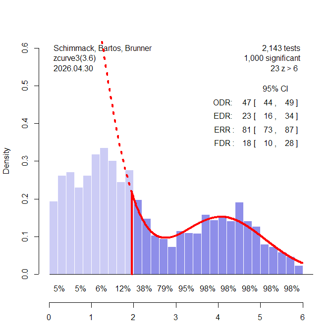
Sometime in the wake of the replication crisis around 2014/15, I went to his office to talk to him about power and bias detection. . Working with Jerry was educational and motivational. Without him z-curve would not exist. We spend years on trying different methods and thinking about the underlying statistical assumptions. Simulations often shattered our intuitions. The Brunner and Schimmack (2020) article summarizes all of this work.
A few years later, the method is being used to examine the credibility of published articles across different research areas. However, not everybody is happy about a tool that can reveal publication bias, the use of questionable research practices, and a high risk of false positive results. An anonymous reviewer dismissed z-curve results based on a long list of criticisms (Post: Dear Anonymous Reviewer). It was funny to see how ChatGPT responds to these criticisms (Comment). However, the quality of ChatGPT responses is difficult to evaluate. Therefore, I am pleased to share Jerry’s response to the reviewer’s comments here. Let’s just say that the reviewer was wise to make their comments anonymously. Posting the review and the response in public also shows why we need open reviews like the ones published in Meta-Psychology by the reviewers of our z-curve article. Hidden and biased reviews are just one more reason why progress in psychology is so slow.
Jerry Brunner’s Response
This is Jerry Brunner, the “Professor of Statistics” mentioned the post. I am also co-author of Brunner and Schimmack (2020). Since the review Uli posted is mostly an attack on our joint paper (Brunner and Schimmack, 2020), I thought I’d respond.
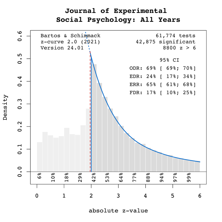
First of all, z-curve is sort of a moving target. The method described by Brunner and Schimmack is strictly a way of estimating population mean power based on a random sample of tests that have been selected for statistical significance. I’ll call it z-curve 1.0. The algorithm has evolved over time, and the current z-curve R package (available at https://cran.r-project.org/web/packages/zcurve/index.html) implements a variety of diagnostics based on a sample of p-values. The reviewer’s comments apply to z-curve 1.0, and so do my responses. This is good from my perspective, because I was in on the development of z-curve 1.0, and I believe I understand it pretty well. When I refer to z-curve in the material that follows, I mean z-curve 1.0. I do believe z-curve 1.0 has some limitations, but they do not overlap with the ones suggested by the reviewer.
Here are some quotes from the review, followed by my answers.
(1) “… z-curve analysis is based on the concept of using an average power estimate of completed studies (i.e., post hoc power analysis). However, statisticians and methodologists have written about the problem of post hoc power analysis …”
This is not accurate. Post-hoc power analysis is indeed fatally flawed; z-curve is something quite different. For later reference, in the “observed” power method, sample effect size is used to estimate population effect size for a single study. Estimated effect size is combined with observed sample size to produce an estimated non-centrality parameter for the non-central distribution of the test statistic, and estimated power is calculated from that, as an area under the curve of the non-central distribution. So, the observed power method produces an estimated power for an individual study. These estimates have been found to be too noisy for practical use.
The confusion of z-curve with observed power comes up frequently in the reviewer’s comments. To be clear, z-curve does not estimate effect sizes, nor does it produce power estimates for individual studies.
(2) “It should be noted that power is not a property of a (completed) study (fixed data). Power is a performance measure of a procedure (statistical test) applied to an infinite number of studies (random data) represented by a sampling distribution. Thus, what one estimates from completed study is not really “power” that has the properties of a frequentist probability even though the same formula is used. Average power does not solve this ontological problem (i.e., misunderstanding what frequentist probability is; see also McShane et al., 2020). Power should always be about a design for future studies, because power is the probability of the performance of a test (rejecting the null hypothesis) over repeated samples for some specified sample size, effect size, and Type I error rate (see also Greenland et al., 2016; O’Keefe, 2007). z-curve, however, makes use of this problematic concept of average power (for completed studies), which brings to question the validity of z-curve analysis results.”
The reviewer appears to believe that once the results of a study are in, the study no longer has a power. To clear up this misconception, I will describe the model on which z-curve is based.
There is a population of studies, each with its own subject population. One designated significance test will be carried out on the data for each study. Given the subject population, the procedure and design of the study (including sample size), significance level and the statistical test employed, there is a probability of rejecting the null hypothesis. This probability has the usual frequentist interpretation; it’s the long-term relative frequency of rejection based on (hypothetical) repeated sampling from the particular subject population. I will use the term “power” for the probability of rejecting the null hypothesis, whether or not the null hypothesis is exactly true.
Note that the power of the test — again, a member of a population of tests — is a function of the design and procedure of the study, and also of the true state of affairs in the subject population (say, as captured by effect size).
So, every study in the population of studies has a power. It’s the same before any data are collected, and after the data are collected. If the study were replicated exactly with a fresh sample from the same population, the probability of observing significant results would be exactly the power of the study — the true power.
This takes care of the reviewer’s objection, but let me continue describing our model, because the details will be useful later.
For each study in the population of studies, a random sample is drawn from the subject population, and the null hypothesis is tested. The results are either significant, or not. If the results are not significant, they are rejected for publication, or more likely never submitted. They go into the mythical “file drawer,” and are no longer available. The studies that do obtain significant results form a sub-population of the original population of studies. Naturally, each of these studies has a true power value. What z-curve is trying to estimate is the population mean power of the studies with significant results.
So, we draw a random sample from the population of studies with significant results, and use the reported results to estimate population mean power — not of the original population of studies, but only of the subset that obtained significant results. To us, this roughly corresponds to the mean power in a population of published results in a particular field or sub-field.
Note that there are two sources of randomness in the model just described. One arises from the random sampling of studies, and the other from random sampling of subjects within studies. In an appendix containing the theorems, Brunner and Schimmack liken designing a study (and choosing a test) to the manufacture of a biased coin with probability of heads equal to the power. All the coins are tossed, corresponding to running the subjects, collecting the data and carrying out the tests. Then the coins showing tails are discarded. We seek to estimate the mean P(Head) for all the remaining coins.
(3) “In Brunner and Schimmack (2020), there is a problem with ‘Theorem 1 states that success rate and mean power are equivalent …’ Here, the coin flip with a binary outcome is a process to describe significant vs. nonsignificant p-values. Focusing on observed power, the problem is that using estimated effect sizes (from completed studies) have sampling variability and cannot be assumed to be equivalent to the population effect size.”
There is no problem with Theorem 1. The theorem says that in the coin tossing experiment just described, suppose you (1) randomly select a coin from the population, and (2) toss it — so there are two stages of randomness. Then the probability of observing a head is exactly equal to the mean P(Heads) for the entire set of coins. This is pretty cool if you think about it. The theorem makes no use of the concept of effect size. In fact, it’s not directly about estimation at all; it’s actually a well-known result in pure probability, slightly specialized for this setting. The reviewer says “Focusing on observed power …” But why would he or she focus on observed power? We are talking about true power here.
(4) “Coming back to p-values, these statistics have their own distribution (that cannot be derived unless the effect size is null and the p-value follows a uniform distribution).
They said it couldn’t be done. Actually, deriving the distribution of the p-value under the alternative hypothesis is a reasonable homework problem for a masters student in statistics. I could give some hints …
(5) “Now, if the counter argument taken is that z-curve does not require an effect size input to calculate power, then I’m not sure what z-curve calculates because a value of power is defined by sample size, effect size, Type I error rate, and the sampling distribution of the statistical procedure (as consistently presented in textbooks for data analysis).”
Indeed, z-curve uses only p-values, from which useful estimates of effect size cannot be recovered. As previously stated, z-curve does not estimate power for individual studies. However, the reviewer is aware that p-values have a probability distribution. Intuitively, shouldn’t the distribution of p-values and the distribution of power values be connected in some way? For example, if all the null hypotheses in a population of tests were true so that all power values were equal to 0.05, then the distribution of p-values would be uniform on the interval from zero to one. When the null hypothesis of a test is false, the distribution of the p-value is right skewed and strictly decreasing (except in pathological artificial cases), with more of the probability piling up near zero. If average power were very high, one might expect a distribution with a lot of very small p-values. The point of this is just that the distribution of p-values surely contains some information about the distribution of power values. What z-curve does is to massage a sample of significant p-values to produce an estimate, not of the entire distribution of power after selection, but just of its population mean. It’s not an unreasonable enterprise, in spite of what the reviewer thinks. Also, it works well for large samples of studies. This is confirmed in the simulation studies reported by Brunner and Schimmack.
(6) “The problem of Theorem 2 in Brunner and Schimmack (2020) is assuming some distribution of power (for all tests, effect sizes, and sample sizes). This is curious because the calculation of power is based on the sampling distribution of a specific test statistic centered about the unknown population effect size and whose variance is determined by sample size. Power is then a function of sample size, effect size, and the sampling distribution of the test statistic.”
Okay, no problem. As described above, every study in the population of studies has its own test statistic, its own true (not estimated) effect size, its own sample size — and therefore its own true power. The relative frequency histogram of these numbers is the true population distribution of power.
(7) “There is no justification (or mathematical derivation) to show that power follows a uniform or beta distribution (e.g., see Figure 1 & 2 in Brunner and Schimmack, 2000, respectively).”
Right. These were examples, illustrating the distribution of power before versus after selection for significance — as given in Theorem 2. Theorem 2 applies to any distribution of true power values.
(8) “If the counter argument here is that we avoid these issues by transforming everything into a z-score, there is no justification that these z-scores will follow a z-distribution because the z-score is derived from a normal distribution – it is not the transformation of a p-value that will result in a z-distribution of z-scores … it’s weird to assume that p-values transformed to z-scores might have the standard error of 1 according to the z-distribution …”
The reviewer is objecting to Step 1 of constructing a z-curve estimate, given on page 6 of Brunner and Schimmack (2020). We start with a sample of significant p-values, arising from a variety of statistical tests, various F-tests, chi-squared tests, whatever — all with different sample sizes. Then we pretend that all the tests were actually two-sided z-tests with the results in the predicted direction, equivalent to one-sided z-tests with significance level 0.025. Then we transform the p-values to obtain the z statistics that would have generated them, had they actually been z-tests. Then we do some other stuff to the z statistics.
But as the reviewer notes, most of the tests probably are not z-tests. The distributions of their p-values, which depend on the non-central distributions of their test statistics, are different from one another, and also different from the distribution for genuine z-tests. Our paper describes it as an approximation, but why should it be a good approximation? I honestly don’t know, and I have given it a lot of thought. I certainly would not have come up with this idea myself, and when Uli proposed it, I did not think it would work. We both came up with a lot of estimation methods that did not work when we tested them out. But when we tested this one, it was successful. Call it a brilliant leap of intuition on Uli’s part. That’s how I think of it.
Uli’s comment.
It helps to know your history. Well before psychologists focused on effect sizes for meta-analysis, Fisher already had a method to meta-analyze p-values. P-Curve is just a meta-analysis of p-values with a selection model. However, p-values have ugly distributions and Stouffer proposed the transformation of p-values into z-scores to conduct meta-analyses. This method was used by Rosenthal to compute the fail-safe-N, one of the earliest methods to evaluate the credibility of published results (Fail-Safe-N). Ironically, even the p-curve app started using this transformation (p-curve changes). Thus, p-curve is really a version of z-curve. The problem with p-curve is that it has only one parameter and cannot model heterogeneity in true power. This is the key advantage of z-curve.1.0 over p-curve (Brunner & Schimmack, 2020). P-curve is even biased when all studies have the same population effect size, but different sample sizes, which leads to heterogeneity in power (Brunner, 2018].
Such things are fairly common in statistics. An idea is proposed, and it seems to work. There’s a “proof,” or at least an argument for the method, but the proof does not hold up. Later on, somebody figures out how to fill in the missing technical details. A good example is Cox’s proportional hazards regression model in survival analysis. It worked great in a large number of simulation studies, and was widely used in practice. Cox’s mathematical justification was weak. The justification starts out being intuitively reasonable but not quite rigorous, and then deteriorates. I have taught this material, and it’s not a pleasant experience. People used the method anyway. Then decades after it was proposed by Cox, somebody else (Aalen and others) proved everything using a very different and advanced set of mathematical tools. The clean justification was too advanced for my students.
Another example (from mathematics) is Fermat’s last theorem, which took over 300 years to prove. I’m not saying that z-curve is in the same league as Fermat’s last theorem, just that statistical methods can be successful and essentially correct before anyone has been able to provide a rigorous justification.
Still, this is one place where the reviewer is not completely mixed up.
Another Uli comment
Undergraduate students are often taught different test statistics and distributions as if they are totally different. However, most tests in psychology are practically z-tests. Just look at a t-distribution with N = 40 (df = 38) and try to see the difference to a standard normal distribution. The difference is tiny and invisible when you increase sample sizes above 40! And F-tests. F-values with 1 experimenter degree of freedom are just squared t-values, so the square root of these is practically a z-test. But what about chi-square? Well, with 1 df, chi-square is just a squared z-score, so we can use the square root and have a z-score. But what if we don’t have two groups, but compute correlations or regressions? Well, the statistical significance test uses the t-distribution and sample sizes are often well above 40. So, t and z are practically identical. It is therefore not surprising to me that approximating empirical results with different test-statistics can be approximated with the standard normal distribution. We could make teaching statistics so much easier, instead of confusing students with F-distributions. The only exception are complex designs with 3 x 4 x 5 ANOVAs, but they don’t really test anything and are just used to p-hack. Rant over. Back to Jerry.
(9) “It is unclear how Theorem 2 is related to the z-curve procedure.”
Theorem 2 is about how selection for significance affects the probability distribution of true power values. Z-curve estimates are based only on studies that have achieved significant results; the others are hidden, by a process that can be called publication bias. There is a fundamental distinction between the original population of power values and the sub-population belonging to studies that produce significant results. The theorems in the appendix are intended to clarify that distinction. The reviewer believes that once significance has been observed, the studies in question no longer even have true power values. So, clarification would seem to be necessary.
(10) “In the description of the z-curve analysis, it is unclear why z-curve is needed to calculate “average power.” If p < .05 is the criterion of significance, then according to Theorem 1, why not count up all the reported p-values and calculate the proportion in which the p-values are significant?”
If there were no selection for significance, this is what a reasonable person would do. But the point of the paper, and what makes the estimation problem challenging, is that all we can observe are statistics from studies with p < 0.05. Publication bias is real, and z-curve is designed to allow for it.
(11) “To beat a dead horse, z-curve makes use of the concept of “power” for completed studies. To claim that power is a property of completed studies is an ontological error …”
Wrong. Power is a feature of the design of a study, the significance test, and the subject population. All of these features still exist after data have been collected and the test is carried out.
Uli and Jerry comment:
Whenever a psychologist uses the word “ontological,” be very skeptical. Most psychologists who use the word understand philosophy as well as this reviewer understands statistics.
(12) “The authors make a statement that (observed) power is the probability of exact replication. However, there is a conceptual error embedded in this statement. While Greenwald et al. (1996, p. 1976) state “replicability can be computed as the power of an exact replication study, which can be approximated by [observed power],” they also explicitly emphasized that such a statement requires the assumption that the estimated effect size is the same as the unknown population effect size which they admit cannot be met in practice.”
Observed power (a bad estimate of true power) is not the probability of significance upon exact replication. True power is the probability of significance upon exact replication. It’s based on true effect size, not estimated effect size. We were talking about true power, and we mistakenly thought that was obvious.
(13) “The basis of supporting the z-curve procedure is a simulation study. This approach merely confirms what is assumed with simulation and does not allow for the procedure to be refuted in any way (cf. Popper’s idea of refutation being the basis of science.) In a simulation study, one assumes that the underlying process of generating p-values is correct (i.e., consistent with the z-curve procedure). However, one cannot evaluate whether the p-value generating process assumed in the simulation study matches that of empirical data. Stated a different way, models about phenomena are fallible and so we find evidence to refute and corroborate these models. The simulation in support of the z-curve does not put the z-curve to the test but uses a model consistent with the z-curve (absent of empirical data) to confirm the z-curve procedure (a tautological argument). This is akin to saying that model A gives us the best results, and based on simulated data on model A, we get the best results.”
This criticism would have been somewhat justified if the simulations had used p-values from a bunch of z-tests. However, they did not. The simulations reported in the paper are all F-tests with one numerator degree of freedom, and denominator degrees of freedom depending on the sample size. This covers all the tests of individual regression coefficients in multiple regression, as well as comparisons of two means using two-sample (and even matched) t-tests. Brunner and Schmmack say (p. 8)
Because the pattern of results was similar for F-tests
and chi-squared tests and for different degrees of freedom,
we only report details for F-tests with one numerator
degree of freedom; preliminary data mining of
the psychological literature suggests that this is the case
most frequently encountered in practice. Full results are
given in the supplementary materials.
So I was going to refer the reader (and the anonymous reviewer, who is probably not reading this post anyway) to the supplementary materials. Fortunately I checked first, and found that the supplementary materials include a bunch of OSF stuff like the letter submitting the article for publication, and the reviewers’ comments and so on — but not the full set of simulations. Oops.
All the code and the full set of simulation results is posted at
https://www.utstat.utoronto.ca/brunner/zcurve2018
You can download all the material in a single file at
https://www.utstat.utoronto.ca/brunner/zcurve2018.zip
After expanding, just open index.html in a browser.
Actually we did a lot more simulation studies than this, but you have to draw the line somewhere. The point is that z-curve performs well for large numbers of studies with chi-squared test statistics as well as F statistics — all with varying degrees of freedom.
(14) “The simulation study was conducted for the performance of the z-curve on constrained scenarios including F-tests with df = 1 and not for the combination of t-tests and chi-square tests as applied in the current study. I’m not sure what to make of the z-curve performance for the data used in the current paper because the simulation study does not provide evidence of its performance under these unexplored conditions.”
Now the reviewer is talking about the paper that was actually under review. The mistake is natural, because of our (my) error in not making sure that the full set of simulations was included in the supplementary materials. The conditions in question are not unexplored; they are thoroughly explored, and the accuracy of z-curve for large samples is confirmed.
(15+) There are some more comments by the reviewer, but these are strictly about the paper under review, and not about Brunner and Schimmack (2020). So, I will leave any further response to others.