THEORETICAL BACKGROUND
Neyman & Pearson (1933) developed the theory of type-I and type-II errors in statistical hypothesis testing.
A type-I error is defined as the probability of rejecting the null-hypothesis (i.e., the effect size is zero) when the null-hypothesis is true.
A type-II error is defined as the probability of failing to reject the null-hypothesis when the null-hypothesis is false (i.e., there is an effect).
A common application of statistics is to provide empirical evidence for a theoretically predicted relationship between two variables (cause-effect or covariation). The results of an empirical study can produce two outcomes. Either the result is statistically significant or it is not statistically significant. Statistically significant results are interpreted as support for a theoretically predicted effect.
Statistically non-significant results are difficult to interpret because the prediction may be false (the null-hypothesis is true) or a type-II error occurred (the theoretical prediction is correct, but the results fail to provide sufficient evidence for it).
To avoid type-II errors, researchers can design studies that reduce the type-II error probability. The probability of avoiding a type-II error when a predicted effect exists is called power. It could also be called the probability of success because a significant result can be used to provide empirical support for a hypothesis.
Ideally researchers would want to maximize power to avoid type-II errors. However, powerful studies require more resources. Thus, researchers face a trade-off between the allocation of resources and their probability to obtain a statistically significant result.
Jacob Cohen dedicated a large portion of his career to help researchers with the task of planning studies that can produce a successful result, if the theoretical prediction is true. He suggested that researchers should plan studies to have 80% power. With 80% power, the type-II error rate is still 20%, which means that 1 out of 5 studies in which a theoretical prediction is true would fail to produce a statistically significant result.
Cohen (1962) examined the typical effect sizes in psychology and found that the typical effect size for the mean difference between two groups (e.g., men and women or experimental vs. control group) is about half-of a standard deviation. The standardized effect size measure is called Cohen’s d in his honor. Based on his review of the literature, Cohen suggested that an effect size of d = .2 is small, d = .5 moderate, and d = .8. Importantly, a statistically small effect size can have huge practical importance. Thus, these labels should not be used to make claims about the practical importance of effects. The main purpose of these labels is that researchers can better plan their studies. If researchers expect a large effect (d = .8), they need a relatively small sample to have high power. If researchers expect a small effect (d = .2), they need a large sample to have high power. Cohen (1992) provided information about effect sizes and sample sizes for different statistical tests (chi-square, correlation, ANOVA, etc.).
Cohen (1962) conducted a meta-analysis of studies published in a prominent psychology journal. Based on the typical effect size and sample size in these studies, Cohen estimated that the average power in studies is about 60%. Importantly, this also means that the typical power to detect small effects is less than 60%. Thus, many studies in psychology have low power and a high type-II error probability. As a result, one would expect that journals often report that studies failed to support theoretical predictions. However, the success rate in psychological journals is over 90% (Sterling, 1959; Sterling, Rosenbaum, & Weinkam, 1995). There are two explanations for discrepancies between the reported success rate and the success probability (power) in psychology. One explanation is that researchers conduct multiple studies and only report successful studies. The other studies remain unreported in a proverbial file-drawer (Rosenthal, 1979). The other explanation is that researchers use questionable research practices to produce significant results in a study (John, Loewenstein, & Prelec, 2012). Both practices have undesirable consequences for the credibility and replicability of published results in psychological journals.
A simple solution to the problem would be to increase the statistical power of studies. If the power of psychological studies in psychology were over 90%, a success rate of 90% would be justified by the actual probability of obtaining significant results. However, meta-analysis and method articles have repeatedly pointed out that psychologists do not consider statistical power in the planning of their studies and that studies continue to be underpowered (Maxwell, 2004; Schimmack, 2012; Sedlmeier & Giegerenzer, 1989).
One reason for the persistent neglect of power could be that researchers have no awareness of the typical power of their studies. This could happen because observed power in a single study is an imperfect indicator of true power (Yuan & Maxwell, 2005). If a study produced a significant result, the observed power is at least 50%, even if the true power is only 30%. Even if the null-hypothesis is true, and researchers publish only type-I errors, observed power is dramatically inflated to 62%, when the true power is only 5% (the type-I error rate). Thus, Cohen’s estimate of 60% power is not very reassuring.
Over the past years, Schimmack and Brunner have developed a method to estimate power for sets of studies with heterogeneous designs, sample sizes, and effect sizes. A technical report is in preparation. The basic logic of this approach is to convert results of all statistical tests into z-scores using the one-tailed p-value of a statistical test. The z-scores provide a common metric for observed statistical results. The standard normal distribution predicts the distribution of observed z-scores for a fixed value of true power. However, for heterogeneous sets of studies the distribution of z-scores is a mixture of standard normal distributions with different weights attached to various power values. To illustrate this method, the histograms of z-scores below show simulated data with 10,000 observations with varying levels of true power: 20% null-hypotheses being true (5% power), 20% of studies with 33% power, 20% of studies with 50% power, 20% of studies with 66% power, and 20% of studies with 80% power.
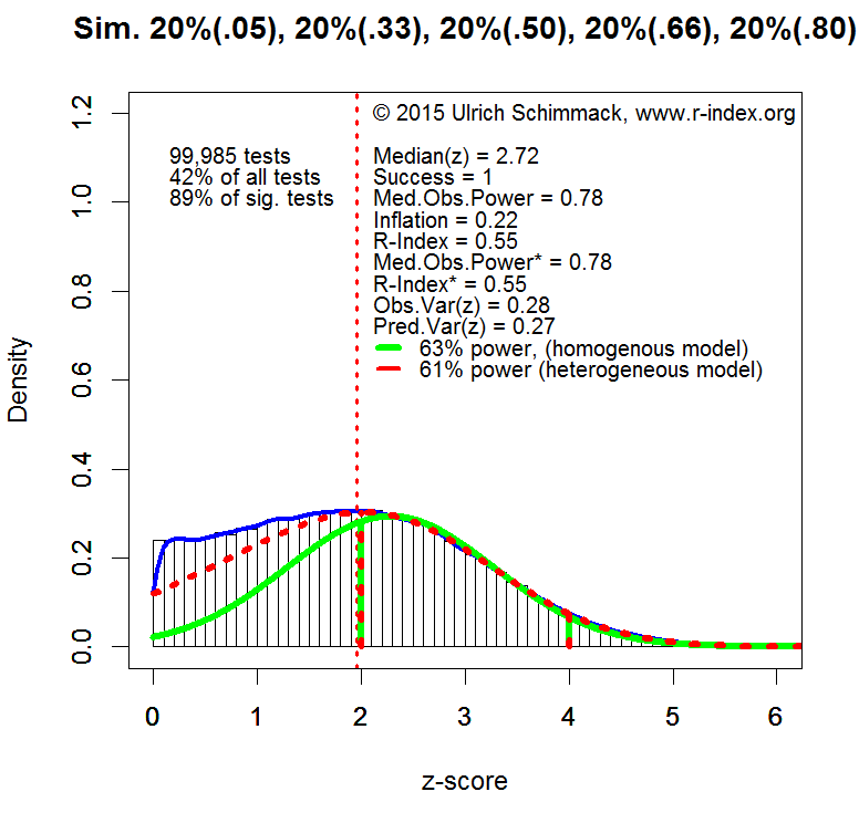
The plot shows the distribution of absolute z-scores (there are no negative effect sizes). The plot is limited to z-scores below 6 (N = 99,985 out of 10,000). Z-scores above 6 standard deviations from zero are extremely unlikely to occur by chance. Even with a conservative estimate of effect size (lower bound of 95% confidence interval), observed power is well above 99%. Moreover, quantum physics uses Z = 5 as a criterion to claim success (e.g., discovery of Higgs-Boson Particle). Thus, Z-scores above 6 can be expected to be highly replicable effects.
Z-scores below 1.96 (the vertical dotted red line) are not significant for the standard criterion of (p < .05, two-tailed). These values are excluded from the calculation of power because these results are either not reported or not interpreted as evidence for an effect. It is still important to realize that true power of all experiments would be lower if these studies were included because many of the non-significant results are produced by studies with 33% power. These non-significant results create two problems. Researchers wasted resources on studies with inconclusive results and readers may be tempted to misinterpret these results as evidence that an effect does not exist (e.g., a drug does not have side effects) when an effect is actually present. In practice, it is difficult to estimate power for non-significant results because the size of the file-drawer is difficult to estimate.
It is possible to estimate power for any range of z-scores, but I prefer the range of z-scores from 2 (just significant) to 4. A z-score of 4 has a 95% confidence interval that ranges from 2 to 6. Thus, even if the observed effect size is inflated, there is still a high chance that a replication study would produce a significant result (Z > 2). Thus, all z-scores greater than 4 can be treated as cases with 100% power. The plot also shows that conclusions are unlikely to change by using a wider range of z-scores because most of the significant results correspond to z-scores between 2 and 4 (89%).
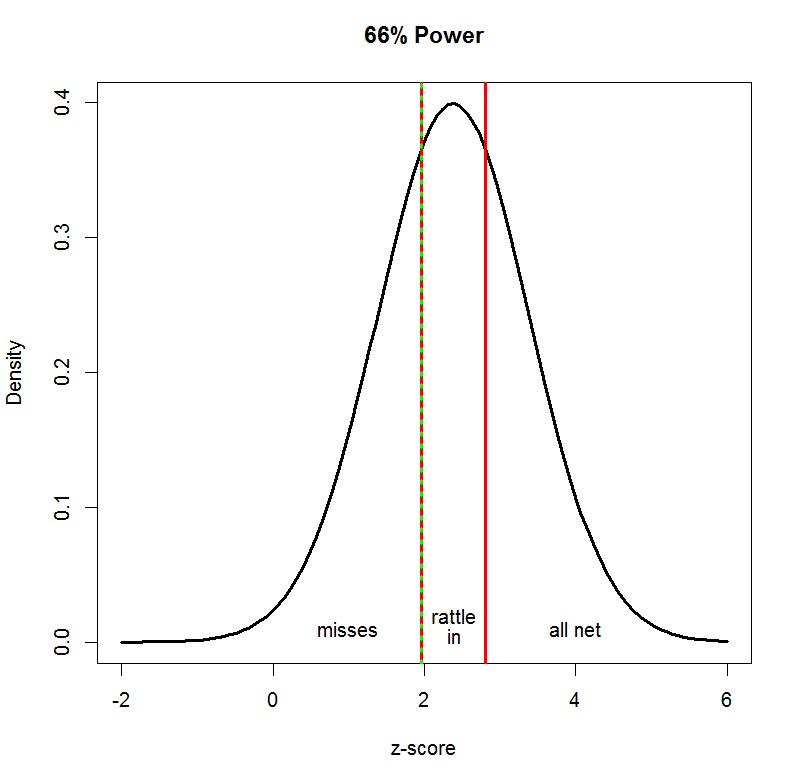
The typical power of studies is estimated based on the distribution of z-scores between 2 and 4. A steep decrease from left to right suggests low power. A steep increase suggests high power. If the peak (mode) of the distribution were centered over Z = 2.8, the data would conform to Cohen’s recommendation to have 80% power.
Using the known distribution of power to estimate power in the critical range gives a power estimate of 61%. A simpler model that assumes a fixed power value for all studies produces a slightly inflated estimate of 63%. Although the heterogeneous model is correct, the plot shows that the homogeneous model provides a reasonable approximation when estimates are limited to a narrow range of Z-scores. Thus, I used the homogeneous model to estimate the typical power of significant results reported in psychological journals.
DATA
The results presented below are based on an ongoing project that examines power in psychological journals (see results section for the list of journals included so far). The set of journals does not include journals that primarily publish reviews and meta-analysis or clinical and applied journals. The data analysis is limited to the years from 2009 to 2015 to provide information about the typical power in contemporary research. Results regarding historic trends will be reported in a forthcoming article.
I downloaded pdf files of all articles published in the selected journals and converted the pdf files to text files. I then extracted all t-tests and F-tests that were reported in the text of the results section searching for t(df) or F(df1,df2). All t and F statistics were converted into one-tailed p-values and then converted into z-scores.

The plot above shows the results based on 218,698 t and F tests reported between 2009 and 2015 in the selected psychology journals. Unlike the simulated data, the plot shows a steep drop for z-scores just below the threshold of significance (z = 1.96). This drop is due to the tendency not to publish or report non-significant results. The heterogeneous model uses the distribution of non-significant results to estimate the size of the file-drawer (unpublished non-significant results). However, for the present purpose the size of the file-drawer is irrelevant because power is estimated only for significant results for Z-scores between 2 and 4.
The green line shows the best fitting estimate for the homogeneous model. The red curve shows fit of the heterogeneous model. The heterogeneous model is doing a much better job at fitting the long tail of highly significant results, but for the critical interval of z-scores between 2 and 4, the two models provide similar estimates of power (55% homogeneous & 53% heterogeneous model). If the range is extended to z-scores between 2 and 6, power estimates diverge (82% homogenous, 61% heterogeneous). The plot indicates that the heterogeneous model fits the data better and that the 61% estimate is a better estimate of true power for significant results in this range. Thus, the results are in line with Cohen (1962) estimate that psychological studies average 60% power.
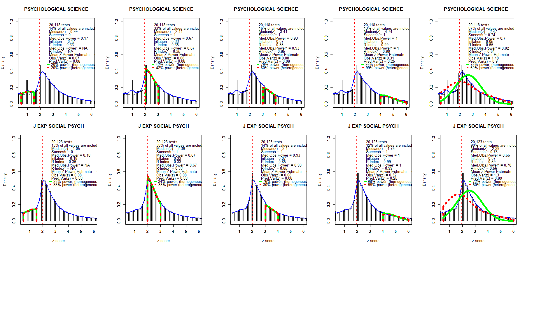
REPLICABILITY RANKING
The distribution of z-scores between 2 and 4 was used to estimate the average power separately for each journal. As power is the probability to obtain a significant result, this measure estimates the replicability of results published in a particular journal if researchers would reproduce the studies under identical conditions with the same sample size (exact replication). Thus, even though the selection criterion ensured that all tests produced a significant result (100% success rate), the replication rate is expected to be only about 50%, even if the replication studies successfully reproduce the conditions of the published studies. The table below shows the replicability ranking of the journals, the replicability score, and a grade. Journals are graded based on a scheme that is similar to grading schemes for undergraduate students (below 50 = F, 50-59 = E, 60-69 = D, 70-79 = C, 80-89 = B, 90+ = A).

The average value in 2000-2014 is 57 (D+). The average value in 2015 is 58 (D+). The correlation for the values in 2010-2014 and those in 2015 is r = .66. These findings show that the replicability scores are reliable and that journals differ systematically in the power of published studies.
LIMITATIONS
The main limitation of the method is that focuses on t and F-tests. The results might change when other statistics are included in the analysis. The next goal is to incorporate correlations and regression coefficients.
The second limitation is that the analysis does not discriminate between primary hypothesis tests and secondary analyses. For example, an article may find a significant main effect for gender, but the critical test is whether gender interacts with an experimental manipulation. It is possible that some journals have lower scores because they report more secondary analyses with lower power. To address this issue, it will be necessary to code articles in terms of the importance of statistical test.
The ranking for 2015 is based on the currently available data and may change when more data become available. Readers should also avoid interpreting small differences in replicability scores as these scores are likely to fluctuate. However, the strong correlation over time suggests that there are meaningful differences in the replicability and credibility of published results across journals.
CONCLUSION
This article provides objective information about the replicability of published findings in psychology journals. None of the journals reaches Cohen’s recommended level of 80% replicability. Average replicability is just about 50%. This finding is largely consistent with Cohen’s analysis of power over 50 years ago. The publication of the first replicability analysis by journal should provide an incentive to editors to increase the reputation of their journal by paying more attention to the quality of the published data. In this regard, it is noteworthy that replicability scores diverge from traditional indicators of journal prestige such as impact factors. Ideally, the impact of an empirical article should be aligned with the replicability of the empirical results. Thus, the replicability index may also help researchers to base their own research on credible results that are published in journals with a high replicability score and to avoid incredible results that are published in journals with a low replicability score. Ultimately, I can only hope that journals will start competing with each other for a top spot in the replicability rankings and as a by-product increase the replicability of published findings and the credibility of psychological science.