To make sense of empirical data, researchers need statistical models, and the choice of model can influence conclusions. It is therefore important to be aware of the assumptions a model makes and, ideally, to test whether those assumptions hold in a particular dataset. This simple truth applies even to the choice of how to describe the average of a variable. As most students learn in a first statistics course, the mean and the median are interchangeable for symmetric distributions but not for skewed ones. In that example, the assumption is easy to check: test the symmetry of the data and pick the better summary.
With more complex models, testing assumptions is harder, and some assumptions cannot be tested at all. In these contexts it is common to leave the influence of assumptions unexamined. It is also awkward to phrase every conclusion as a conditional statement — “assuming the model’s assumptions hold, …” In psychology, correlational researchers are routinely required to flag that any causal claim is conditional on assumptions, or else they are told not to draw conclusions at all. Model-based results, by contrast, are often presented without a careful discussion of the model’s assumptions.
An increasingly popular model for meta-analyses is the step-function selection model (Vevea & Woods, 2005). Like other selection models, it assumes that nonsignificant results often remain unpublished while significant results are published. Other biases may also influence which significant results appear, but most selection models make the simplifying assumption that selection for significance is the key driver of publication bias.
Where selection models differ is in their treatment of nonsignificant results. Models like p-curve and z-curve fit only the significant results and do not condition on the observed nonsignificant ones; they avoid making any assumption about how selection shaped the nonsignificant results. Step-function models instead use the nonsignificant results directly. This can yield more information, but only at the cost of an additional assumption: that the selection process takes a specific form. That extra assumption is the subject of this post — and, as with symmetry and the mean, it is one we can test.
To use non-significant results, step-function models make two assumptions that have to be true to correct for selection bias.
- Non-significant and significant effect size estimates come from the same normal distribution of population effect sizes.
- Selection bias within a step (a range of p-values) is independent of the p-value.
Taken together, these two assumptions make predictions about the observed p-values within a step. This prediction is easier to test when the p-values are converted into z-values. Essentially, selection bias should influence the frequency of results in a step, but not the shape that one would see without selection bias. This prediction has never been tested, but it is possible to do so using a z-curve plot and z-curve analyses of the data.
Here I use actual data from a meta-analysis of Terror Management Studies that used the step-function model (Chen et al., 2025).

A simple histogram of the z-values shows that there are hardly any negative results (Figure 1). However, Chen et al. specified a model that assumes equal selection bias for all z-values between -1.96 and +1.96. Accordingly, the data imply that there really were more non-significant results with a positive effect than a negative effect. This alone implies that the mean of the population effect sizes is positive. Indeed, the model estimated a mean standardized effect size of .347 standard deviations.
An alternative possibility is that there is a stronger selection bias against negative non-significant results than for positive non-significant results. This assumption can be tested by splitting the step at z = 0 (p = .5, one-tailed) and estimating selection bias separately for positive and negative results. This model produces a dramatically different estimate of the average effect size, suggesting that studies, on average, more often produced a negative result (contrary to predictions) than a positive result, standardized mean difference = -.336.
The change in the sign of the estimate shows how sensitive estimates are to model assumptions. I used z-curve (Brunner & Schimmack, 2020; Bartos & Schimmack, 2022) to test the assumption that the distribution of the positive non-significant results is consistent with the assumptions of the step-function model.
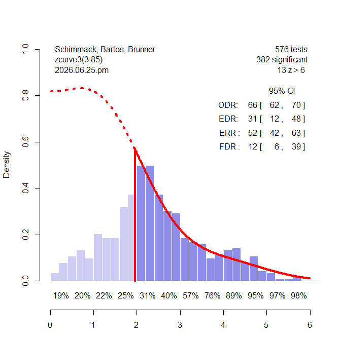
Z-curve fits a finite-mixture model to the distribution of the significant z-values and predicts the distribution of non-significant results from the weights of the mixture components (Figure 2). The z-curve plot shows clear evidence of selection bias. That is there are more observed significant results (66%) than the model predicts (31%). However, the important question is whether the distribution of the non-significant positive z-values matches the predicted distribution shape (the red dotted line in Figure 1).
Visual inspection suggests that this is not the case. There are more observed non-significant results close to the significance criterion than close to zero. In contrast, the predicted pattern shows a flat and then decreasing shape from 0 to 1.65 (values between 1.65 and 1.96 are inconclusive because they are often reported as marginally significant results).
To complement visual inspection with a statistical test, z-curve (version 3.85) compares the distributions while holding the overall density constant (i.e., removing selection bias). A negative difference indicates that there are more z-values close to zero than predicted. A positive difference indicates that there are more z-values close to the significance criterion. A bootstrap confidence interval is used to test for statistical significance.
The median difference was z = .15, 95%CI [ .08, .38]. The mean difference was z = .10, 95%CI = [.05 to .26]. This finding is consistent with the observation that observed z-values close to zero are relatively rare. In short, the observed distribution of the non-significant results is inconsistent with at least one of the assumptions of the step-function model.
The test does not reveal which assumption is violated, and in these data both may be. The depletion of nonsignificant results near zero suggests that selection bias varies within the step, contrary to the assumption that selection is constant within a p-value range. Separately, the near-absence of negative results is hard to reconcile with the model’s estimate of large heterogeneity (tau = .96), which produces a prediction interval for population effect sizes from d = −2.20 to 1.54. A lower bound of −2.20 implies that a substantial share of studies have true effects opposite to the prediction — that mortality primes often produce the reverse of the expected effect. That is implausible; more likely, the negative tail is an artifact of assuming a normal distribution. The shape test cannot identify the true distribution of population effect sizes, but it forces meta-analysts to confront the distribution assumption rather than leave it implicit.
To demonstrate that the shape test works, I used the model weights of the actual data to simulate data without publication bias. I then removed 70% of the non-significant results without changing the distribution of the non-significant results (Figure 2).
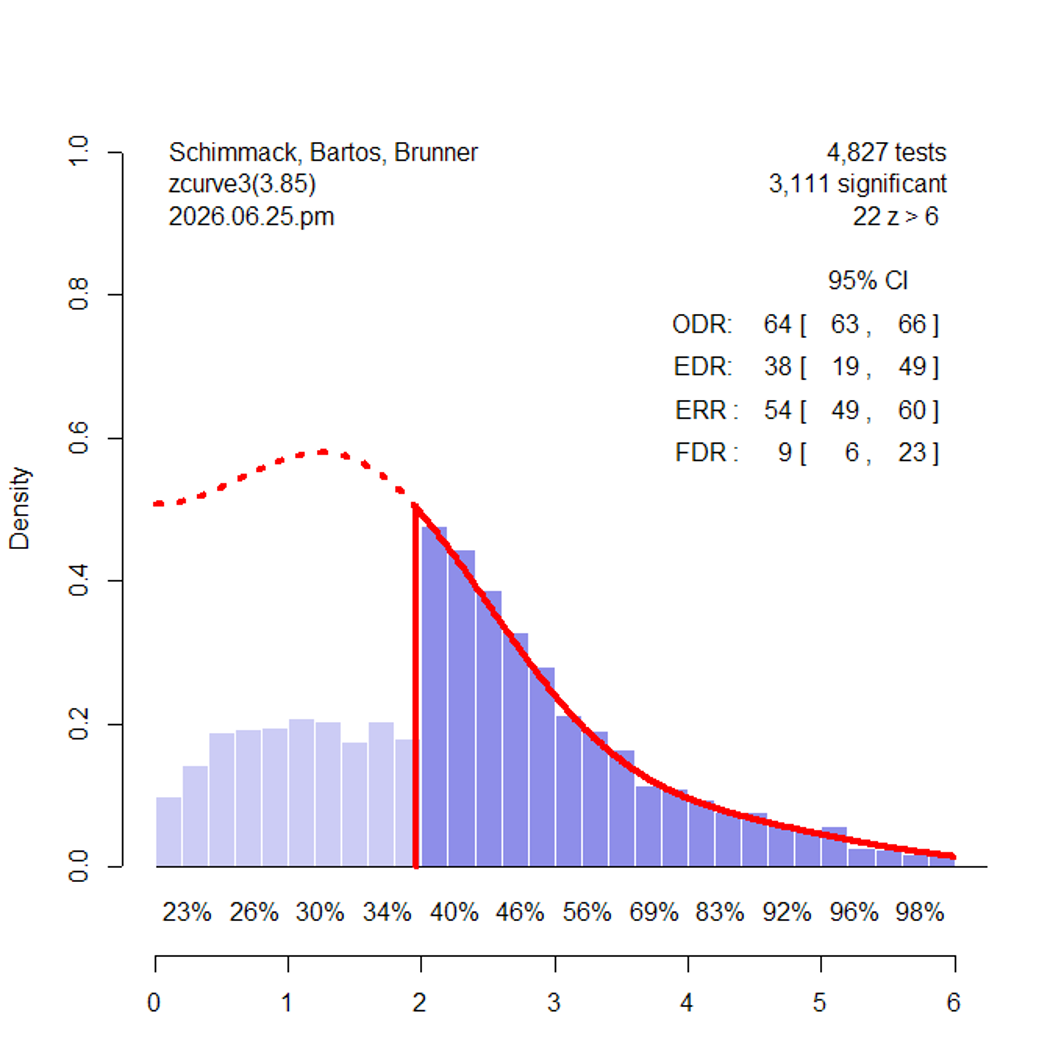
Visual inspection shows that the distribution of the non-significant results is more similar to the predicted distribution. The shape test results are consistent with this observation. The median difference is -.05, 95%CI [-.10, .18]. The mean difference is -.04, 95%CI [-.07, .12]. Both confidence intervals include zero.
In sum, step-function models make assumptions about the distribution of population effect sizes and the selection of non-significant results to use observed non-significant results in the estimation of the amount of bias and the average and standard deviation of the population effect sizes. The advantage is that more data reduce random sampling error. The disadvantage is that violations of assumptions can introduce systematic biases. This disadvantage has been neglected in applications of step-function selection models. The ability to test the assumptions has several benefits. First, it draws more attention to the fact that assumptions influence model estimates. Second, shape tests help readers to evaluate the plausibility of the model and to question estimates that are based on data that are inconsistent with assumptions. Third, assumption tests can resolve inconsistencies between estimates obtained with different models. Results based on models that make fewer assumptions or pass assumption tests are more credible than those based on models that do not meet assumptions.
In conclusion, meta-analysts have many tools to analyze their data that often produce inconsistent results. To make sense of these inconsistencies, it is important to understand why they produce inconsistent results. Violated assumptions are one plausible reason and undermine the plausibility of results of these models.