Tag Archives: r-index

Replicability of Research in Frontiers of Psychology

Summary

The z-curve analysis of results in this journal shows (a) that many published results are based on studies with low to modest power, (b) selection for significance inflates effect size estimates and the discovery rate of reported results, and (c) there is no evidence that research practices have changed over the past decade. Readers should be careful when they interpret results and recognize that reported effect sizes are likely to overestimate real effect sizes, and that replication studies with the same sample size may fail to produce a significant result again. To avoid misleading inferences, I suggest using alpha = .005 as a criterion for valid rejections of the null-hypothesis. Using this criterion, the risk of a false positive result is below 2%. I also recommend computing a 99% confidence interval rather than the traditional 95% confidence interval for the interpretation of effect size estimates.

Given the low power of many studies, readers also need to avoid the fallacy to report non-significant results as evidence for the absence of an effect. With 50% power, the results can easily switch in a replication study so that a significant result becomes non-significant and a non-significant result becomes significant. However, selection for significance will make it more likely that significant results become non-significant than observing a change in the opposite direction.

The average power of studies in a heterogeneous journal like Frontiers of Psychology provides only circumstantial evidence for the evaluation of results. When other information is available (e.g., z-curve analysis of a discipline, author, or topic, it may be more appropriate to use this information).

Report

Frontiers of Psychology was created in 2010 as a new online-only journal for psychology. It covers many different areas of psychology, although some areas have specialized Frontiers journals like Frontiers in Behavioral Neuroscience.

The business model of Frontiers journals relies on publishing fees of authors, while published articles are freely available to readers.

The number of articles in Frontiers of Psychology has increased quickly from 131 articles in 2010 to 8,072 articles in 2022 (source Web of Science). With over 8,000 published articles Frontiers of Psychology is an important outlet for psychological researchers to publish their work. Many specialized, print-journals publish fewer than 100 articles a year. Thus, Frontiers of Psychology offers a broad and large sample of psychological research that is equivalent to a composite of 80 or more specialized journals.

Another advantage of Frontiers of Psychology is that it has a relatively low rejection rate compared to specialized journals that have limited journal space. While high rejection rates may allow journals to prioritize exceptionally good research, articles published in Frontiers of Psychology are more likely to reflect the common research practices of psychologists.

To examine the replicability of research published in Frontiers of Psychology, I downloaded all published articles as PDF files, converted PDF files to text files, and extracted test-statistics (F, t, and z-tests) from published articles. Although this method does not capture all published results, there is no a priori reason that results reported in this format differ from other results. More importantly, changes in research practices such as higher power due to larger samples would be reflected in all statistical tests.

As Frontiers of Psychology only started shortly before the replication crisis in psychology increased awareness about the problem of low statistical power and selection for significance (publication bias), I was not able to examine replicability before 2011. I also found little evidence of changes in the years from 2010 to 2015. Therefore, I use this time period as the starting point and benchmark for future years.

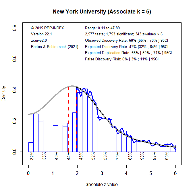
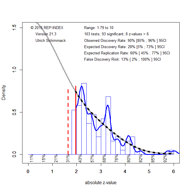
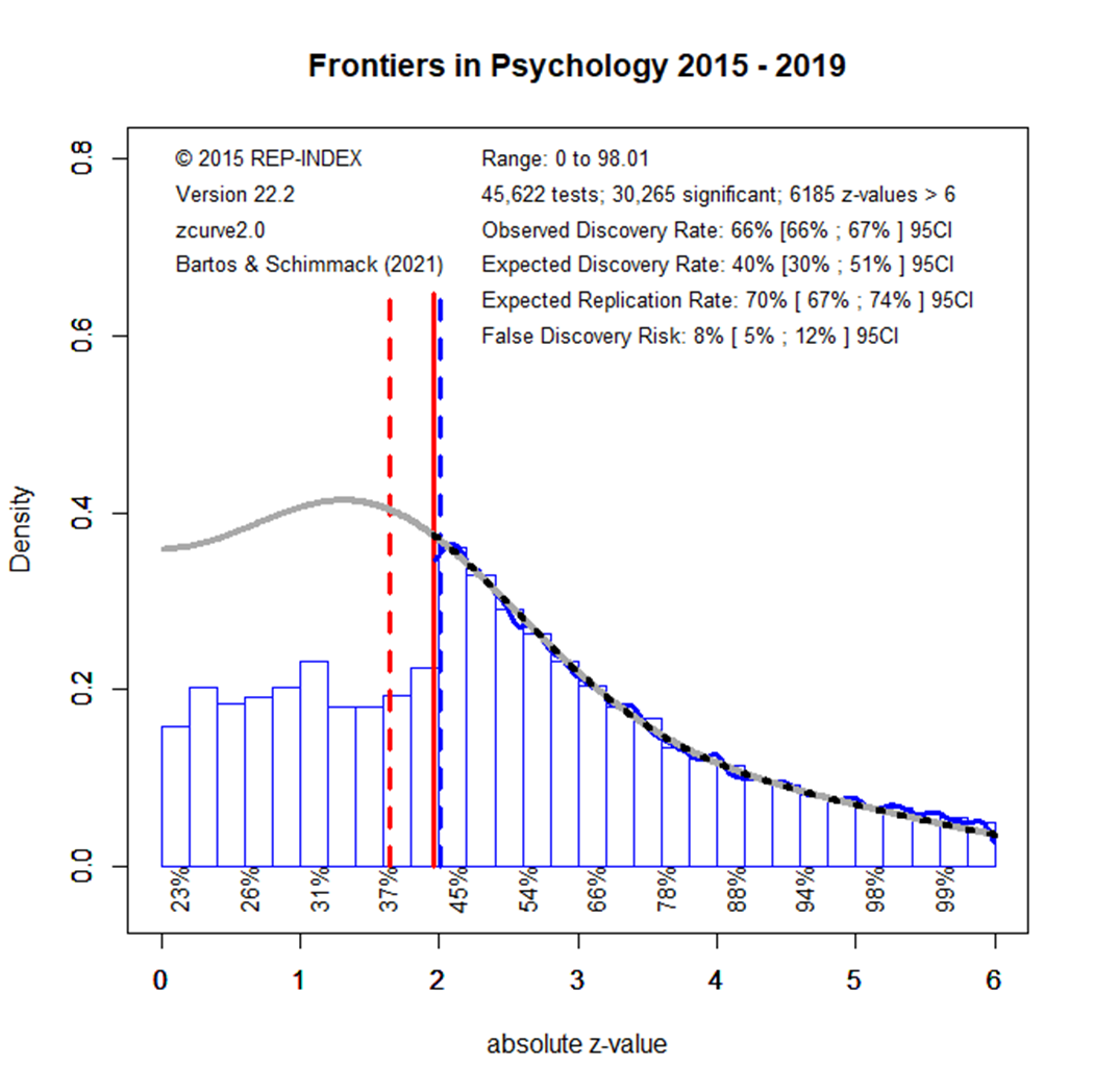
Figure 1 shows a z-curve plot of results published from 2010 to 2014. All test-statistics are converted into z-scores. Z-scores greater than 1.96 (the solid red line) are statistically significant at alpha = .05 (two-sided) and typically used to claim a discovery (rejection of the null-hypothesis). Sometimes even z-scores between 1.65 (the dotted red line) and 1.96 are used to reject the null-hypothesis either as a one-sided test or as marginal significance. Using alpha = .05, the plot shows 71% significant results, which is called the observed discovery rate (ODR).

Visual inspection of the plot shows a peak of the distribution right at the significance criterion. It also shows that z-scores drop sharply on the left side of the peak when the results do not reach the criterion for significance. This wonky distribution cannot be explained with sampling error. Rather it shows a selective bias to publish significant results by means of questionable practices such as not reporting failed replication studies or inflating effect sizes by means of statistical tricks. To quantify the amount of selection bias, z-curve fits a model to the distribution of significant results and estimates the distribution of non-significant (i.e., the grey curve in the range of non-significant results). The discrepancy between the observed distribution and the expected distribution shows the file-drawer of missing non-significant results. Z-curve estimates that the reported significant results are only 31% of the estimated distribution. This is called the expected discovery rate (EDR). Thus, there are more than twice as many significant results as the statistical power of studies justifies (71% vs. 31%). Confidence intervals around these estimates show that the discrepancy is not just due to chance, but active selection for significance.

Using a formula developed by Soric (1989), it is possible to estimate the false discovery risk (FDR). That is, the probability that a significant result was obtained without a real effect (a type-I error). The estimated FDR is 12%. This may not be alarming, but the risk varies as a function of the strength of evidence (the magnitude of the z-score). Z-scores that correspond to p-values close to p =.05 have a higher false positive risk and large z-scores have a smaller false positive risk. Moreover, even true results are unlikely to replicate when significance was obtained with inflated effect sizes. The most optimistic estimate of replicability is the expected replication rate (ERR) of 69%. This estimate, however, assumes that a study can be replicated exactly, including the same sample size. Actual replication rates are often lower than the ERR and tend to fall between the EDR and ERR. Thus, the predicted replication rate is around 50%. This is slightly higher than the replication rate in the Open Science Collaboration replication of 100 studies which was 37%.

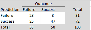
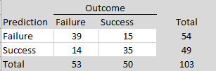
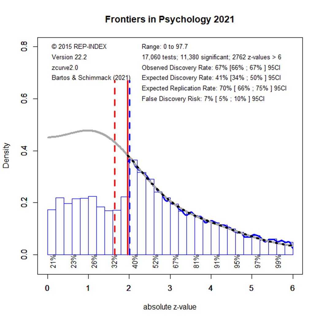
Figure 2 examines how things have changed in the next five years.

The observed discovery rate decreased slightly, but statistically significantly, from 71% to 66%. This shows that researchers reported more non-significant results. The expected discovery rate increased from 31% to 40%, but the overlapping confidence intervals imply that this is not a statistically significant increase at the alpha = .01 level. (if two 95%CI do not overlap, the difference is significant at around alpha = .01). Although smaller, the difference between the ODR of 60% and the EDR of 40% is statistically significant and shows that selection for significance continues. The ERR estimate did not change, indicating that significant results are not obtained with more power. Overall, these results show only modest improvements, suggesting that most researchers who publish in Frontiers in Psychology continue to conduct research in the same way as they did before, despite ample discussions about the need for methodological reforms such as a priori power analysis and reporting of non-significant results.

The results for 2020 show that the increase in the EDR was a statistical fluke rather than a trend. The EDR returned to the level of 2010-2015 (29% vs. 31), but the ODR remained lower than in the beginning, showing slightly more reporting of non-significant results. The size of the file drawer remains large with an ODR of 66% and an EDR of 72%.

The EDR results for 2021 look again better, but the difference to 2020 is not statistically significant. Moreover, the results in 2022 show a lower EDR that matches the EDR in the beginning.

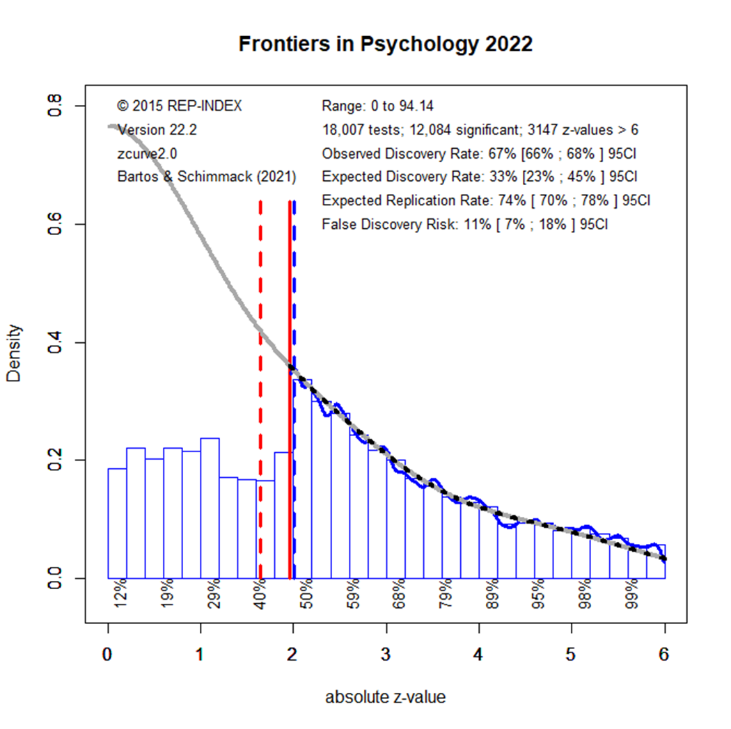
Overall, these results show that results published in Frontiers in Psychology are selected for significance. While the observed discovery rate is in the upper 60%s, the expected discovery rate is around 35%. Thus, the ODR is nearly twice the rate of the power of studies to produce these results. Most concerning is that a decade of meta-psychological discussions about research practices has not produced any notable changes in the amount of selection bias or the power of studies to produce replicable results.

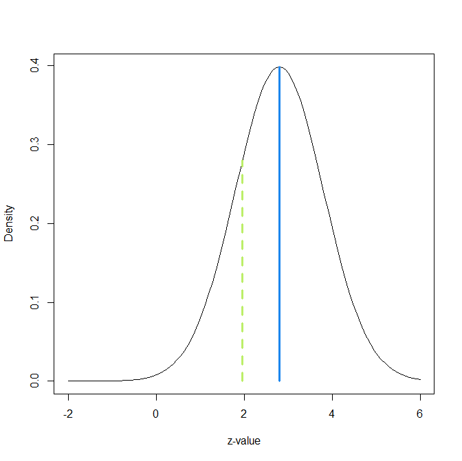
How should readers of Frontiers in Psychology articles deal with this evidence that some published results were obtained with low power and inflated effect sizes that will not replicate? One solution is to retrospectively change the significance criterion. Comparisons of the evidence in original studies and replication outcomes suggest that studies with a p-value below .005 tend to replicate at a rate of 80%, whereas studies with just significant p-values (.050 to .005) replicate at a much lower rate (Schimmack, 2022). Demanding stronger evidence also reduces the false positive risk. This is illustrated in the last figure that uses results from all years, given the lack of any time trend.

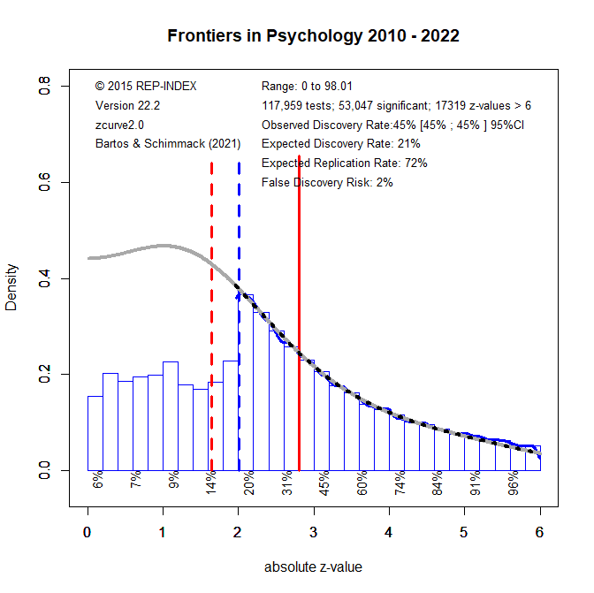
In the Figure the red solid line moved to z = 2.8; the value that corresponds to p = .005, two-sided. Using this more stringent criterion for significance, only 45% of the z-scores are significant. Another 25% were significant with alpha = .05, but are no longer significant with alpha = .005. As power decreases when alpha is set to more stringent, lower, levels, the EDR is also reduced to only 21%. Thus, there is still selection for significance. However, the more effective significance filter also selects for more studies with high power and the ERR remains at 72%, even with alpha = .005 for the replication study. If the replication study used the traditional alpha level of .05, the ERR would be even higher, which explains the finding that the actual replication rate for studies with p < .005 is about 80%.

The lower alpha also reduces the risk of false positive results, even though the EDR is reduced. The FDR is only 2%. Thus, the null-hypothesis is unlikely to be true. The caveat is that the standard null-hypothesis in psychology is the nil-hypothesis and that the population effect size might be too small to be of practical significance. Thus, readers who interpret results with p-values below .005 should also evaluate the confidence interval around the reported effect size, using the more conservative 99% confidence interval that correspondence to alpha = .005 rather than the traditional 95% confidence interval. In many cases, this confidence interval is likely to be wide and provide insufficient information about the strength of an effect.

2021 Replicability Report for the Psychology Department at New York University

Introduction

Since 2011, it is an open secret that many published results in psychology journals do not replicate. The replicability of published results is particularly low in social psychology (Open Science Collaboration, 2015).

A key reason for low replicability is that researchers are rewarded for publishing as many articles as possible without concerns about the replicability of the published findings. This incentive structure is maintained by journal editors, review panels of granting agencies, and hiring and promotion committees at universities.

To change the incentive structure, I developed the Replicability Index, a blog that critically examined the replicability, credibility, and integrity of psychological science. In 2016, I created the first replicability rankings of psychology departments (Schimmack, 2016). Based on scientific criticisms of these methods, I have improved the selection process of articles to be used in departmental reviews.

1. I am using Web of Science to obtain lists of published articles from individual authors (Schimmack, 2022). This method minimizes the chance that articles that do not belong to an author are included in a replicability analysis. It also allows me to classify researchers into areas based on the frequency of publications in specialized journals. Currently, I cannot evaluate neuroscience research. So, the rankings are limited to cognitive, social, developmental, clinical, and applied psychologists.

2. I am using department’s websites to identify researchers that belong to the psychology department. This eliminates articles that are from other departments.

3. I am only using tenured, active professors. This eliminates emeritus professors from the evaluation of departments. I am not including assistant professors because the published results might negatively impact their chances to get tenure. Another reason is that they often do not have enough publications at their current university to produce meaningful results.

Like all empirical research, the present results rely on a number of assumptions and have some limitations. The main limitations are that
(a) only results that were found in an automatic search are included
(b) only results published in 120 journals are included (see list of journals)
(c) published significant results (p < .05) may not be a representative sample of all significant results
(d) point estimates are imprecise and can vary based on sampling error alone.

These limitations do not invalidate the results. Large difference in replicability estimates are likely to predict real differences in success rates of actual replication studies (Schimmack, 2022).

New York University

I used the department website to find core members of the psychology department. I found 13 professors and 6 associate professors. Figure 1 shows the z-curve for all 12,365 tests statistics in articles published by these 19 faculty members. I use the Figure to explain how a z-curve analysis provides information about replicability and other useful meta-statistics.

1. All test-statistics are converted into absolute z-scores as a common metric of the strength of evidence (effect size over sampling error) against the null-hypothesis (typically H0 = no effect). A z-curve plot is a histogram of absolute z-scores in the range from 0 to 6. The 1,239 (~ 10%) of z-scores greater than 6 are not shown because z-scores of this magnitude are extremely unlikely to occur when the null-hypothesis is true (particle physics uses z > 5 for significance). Although they are not shown, they are included in the meta-statistics.

2. Visual inspection of the histogram shows a steep drop in frequencies at z = 1.96 (dashed blue/red line) that corresponds to the standard criterion for statistical significance, p = .05 (two-tailed). This shows that published results are selected for significance. The dashed red/white line shows significance for p < .10, which is often used for marginal significance. There is another drop around this level of significance.

3. To quantify the amount of selection bias, z-curve fits a statistical model to the distribution of statistically significant results (z > 1.96). The grey curve shows the predicted values for the observed significant results and the unobserved non-significant results. The full grey curve is not shown to present a clear picture of the observed distribution. The statistically significant results (including z > 6) make up 20% of the total area under the grey curve. This is called the expected discovery rate because the results provide an estimate of the percentage of significant results that researchers actually obtain in their statistical analyses. In comparison, the percentage of significant results (including z > 6) includes 70% of the published results. This percentage is called the observed discovery rate, which is the rate of significant results in published journal articles. The difference between a 70% ODR and a 20% EDR provides an estimate of the extent of selection for significance. The difference of 50 percentage points is large. The upper level of the 95% confidence interval for the EDR is 28%. Thus, the discrepancy is not just random. To put this result in context, it is possible to compare it to the average for 120 psychology journals in 2010 (Schimmack, 2022). The ODR is similar (70 vs. 72%), but the EDR is a bit lower (20% vs. 28%), although the difference might be largely due to chance.

4. The EDR can be used to estimate the risk that published results are false positives (i.e., a statistically significant result when H0 is true), using Soric’s (1989) formula for the maximum false discovery rate. An EDR of 20% implies that no more than 20% of the significant results are false positives, however the upper limit of the 95%CI of the EDR, 28%, allows for 36% false positive results. Most readers are likely to agree that this is an unacceptably high risk that published results are false positives. One solution to this problem is to lower the conventional criterion for statistical significance (Benjamin et al., 2017). Figure 2 shows that alpha = .005 reduces the point estimate of the FDR to 3% with an upper limit of the 95% confidence interval of XX%. Thus, without any further information readers could use this criterion to interpret results published by NYU faculty members.

5. The estimated replication rate is based on the mean power of significant studies (Brunner & Schimmack, 2020). Under ideal condition, mean power is a predictor of the success rate in exact replication studies with the same sample sizes as the original studies. However, as NYU professor van Bavel pointed out in an article, replication studies are never exact, especially in social psychology (van Bavel et al., 2016). This implies that actual replication studies have a lower probability of producing a significant result, especially if selection for significance is large. In the worst case scenario, replication studies are not more powerful than original studies before selection for significance. Thus, the EDR provides an estimate of the worst possible success rate in actual replication studies. In the absence of further information, I have proposed to use the average of the EDR and ERR as a predictor of actual replication outcomes. With an ERR of 62% and an EDR of 20%, this implies an actual replication prediction of 41%. This is close to the actual replication rate in the Open Science Reproducibility Project (Open Science Collaboration, 2015). The prediction for results published in 120 journals in 2010 was (ERR = 67% + ERR = 28%)/ 2 = 48%. This suggests that results published by NYU faculty are slightly less replicable than the average result published in psychology journals, but the difference is relatively small and might be mostly due to chance.

6. There are two reasons for low replication rates in psychology. One possibility is that psychologists test many false hypotheses (i.e., H0 is true) and many false positive results are published. False positive results have a very low chance of replicating in actual replication studies (i.e. 5% when .05 is used to reject H0), and will lower the rate of actual replications a lot. Alternative, it is possible that psychologists tests true hypotheses (H0 is false), but with low statistical power (Cohen, 1961). It is difficult to distinguish between these two explanations because the actual rate of false positive results is unknown. However, it is possible to estimate the typical power of true hypotheses tests using Soric’s FDR. If 20% of the significant results are false positives, the power of the 80% true positives has to be (.62 – .2*.05)/.8 = 76%. This would be close to Cohen’s recommended level of 80%, but with a high level of false positive results. Alternatively, the null-hypothesis may never be really true. In this case, the ERR is an estimate of the average power to get a significant result for a true hypothesis. Thus, power is estimated to be between 62% and 76%. The main problem is that this is an average and that many studies have less power. This can be seen in Figure 1 by examining the local power estimates for different levels of z-scores. For z-scores between 2 and 2.5, the ERR is only 47%. Thus, many studies are underpowered and have a low probability of a successful replication with the same sample size even if they showed a true effect.

Area

The results in Figure 1 provide highly aggregated information about replicability of research published by NYU faculty. The following analyses examine potential moderators. First, I examined social and cognitive research. Other areas were too small to be analyzed individually.

The z-curve for the 11 social psychologists was similar to the z-curve in Figure 1 because they provided more test statistics and had a stronger influence on the overall result.

The z-curve for the 6 cognitive psychologists looks different. The EDR and ERR are higher for cognitive psychology, and the 95%CI for social and cognitive psychology do not overlap. This suggests systematic differences between the two fields. These results are consistent with other comparisons of the two fields, including actual replication outcomes (OSC, 2015). With an EDR of 44%, the false discovery risk for cognitive psychology is only 7% with an upper limit of the 95%CI at 12%. This suggests that the conventional criterion of .05 does keep the false positive risk at a reasonably low level or that an adjustment to alpha = .01 is sufficient. In sum, the results show that results published by cognitive researchers at NYU are more replicable than those published by social psychologists.

Position

Since 2015 research practices in some areas of psychology, especially social psychology, have changed to increase replicability. This would imply that research by younger researchers is more replicable than research by more senior researchers that have more publications before 2015. A generation effect would also imply that a department’s replicability increases when older faculty members retire. On the other hand, associate professors are relatively young and likely to influence the reputation of a department for a long time.

The figure above shows that most test statistics come from the (k = 13) professors. As a result, the z-curve looks similar to the z-curve for all test values in Figure 1. The results for the 6 associate professors (below) are more interesting. Although five of the six associate professors are in the social area, the z-curve results show a higher EDR and less selection bias than the plot for all social psychologists. This suggests that the department will improve when full professors in social psychology retire.

Some researchers have changed research practices in response to the replication crisis. It is therefore interesting to examine whether replicability of newer research has improved. To examine this question, I performed a z-curve analysis for articles published in the past five year (2016-2021).

The results show very little signs of improvement. The EDR increased from 20% to 26%, but the confidence intervals are too wide to infer that this is a systematic change. In contrast, Stanford University improved from 22% to 50%, a significant increase. For now, NYU results should be interpreted with alpha = .005 as threshold for significance to maintain a reasonable false positive risk.

The table below shows the meta-statistics of all 19 faculty members. You can see the z-curve for each faculty member by clicking on their name.

Rank  NameARPEDRERRFDR
1Karen E. Adolph6676564
2Bob Rehder6175476
3Marjorie Rhodes5868486
4Jay J. van Bavel5566447
5Brian McElree5459496
6David M. Amodio5365408
7Todd M. Gureckis49752317
8Emily Balcetis48682813
9Eric D. Knowles48603510
10Tessa V. West4655379
11Catherine A. Hartley45701923
12Madeline E. Heilman44662318
13John T. Jost44622615
14Andrei Cimpian42642021
15Peter M. Gollwitzer36541825
16Yaacov Trope34541432
17Gabriele Oettingen30461432
18Susan M. Andersen30471335

Predicting Replication Outcomes: Prediction Markets vs. R-Index

Conclusion

Gordon et al. (2021) conducted a meta-analysis of 103 studies that were included in prediction markets to forecast the outcome of replication studies. The results show that prediction markets can forecast replication outcomes above chance levels, but the value of this information is limited. Without actual replication studies, it remains unclear which published results can be trusted or not. Here I compare the performance of prediction markets to the R-Index and the closely related p < .005 rule. These statistical forecasts perform nearly as well as markets and are much easier to use to make sense of thousands of published articles. However, even these methods have a high failure rate. The best solution to this problem is to rely on meta-analyses of studies rather than to predict the outcome of a single study. In addition to meta-analyses, it will be necessary to conduct new studies that are conducted with high scientific integrity to provide solid empirical foundations for psychology. Claims that are not supported by bias-corrected meta-analyses or new preregistered studies are merely suggestive and currently lack empirical support.

Introduction

Since 2011, it became apparent that many published results in psychology, especially social psychology fail to replicate in direct replication studies (Open Science Collaboration, 2015). In social psychology the success rate of replication studies is so low (25%) that it makes sense to bet on replication failures. This would produce 75% successful outcomes, but it would also imply that an entire literature has to be discarded.

It is practically impossible to redo all of the published studies to assess their replicability. Thus, several projects have attempted to predict replication outcomes of individual studies. One strategy is to conduct prediction markets in which participants can earn real money by betting on replication outcomes. There have been four prediction markets with a total of 103 studies with known replication outcomes (Gordon et al., 2021). The key findings are summarized in Table 1.

Markets have a good overall success rate, (28+47)/103 = 73% that is above chance (flipping a coin). Prediction markets are better at predicting failures, 28/31 = 90%, than predicting successes, 47/72 = 65%. The modest success rate for success is a problem because it would be more valuable to be able to identify studies that will replicate and do not require a new study to verify the results.

Another strategy to predict replication outcomes relies on the fact that the p-values of original studies and the p-values of replication studies are influenced by the statistical power of a study (Brunner & Schimmack, 2020). Studies with higher power are more likely to produce lower p-values and more likely to produce significant p-values in replication studies. As a result, p-values also contain valuable information about replication outcomes. Gordon et al. (2021) used p < .005 as a rule to predict replication outcomes. Table 2 shows the performance of this simple rule.

The overall success rate of this rule is nearly as good as the prediction markets, (39+35)/103 = 72%; a difference by k = 1 studies. The rule does not predict failures as well as the markets, 39/54 = 72% (vs. 90%), but it predicts successes slightly better than the markets, 35/49 = 71% (vs. 65%).

A logistic regression analysis showed that both predictors independently contribute to the prediction of replication outcomes, market b = 2.50, se = .68, p = .0002; p < .005 rule: b = 1.44, se = .48, p = .003.

In short, p-values provide valuable information about the outcome of replication studies.

The R-Index

Although a correlation between p-values and replication outcomes follows logically from the influence of power on p-values in original and replication studies, the cut-off value of .005 appears to be arbitrary. Gordon et al. (2017) justify its choice with an article by Benjamin et al. (2017) that recommended a lower significance level (alpha) to ensure a lower false positive risk. Moreover, they advocated for this rule for new studies that preregister hypotheses and do not suffer from selection bias. In contrast, the replication crisis was caused by selection for significance which produced success rates of 90% or more in psychology journals (Motyl et al., 2017; Sterling, 1959; Sterling et al., 1995). One main reason for replication failures is that selection for significance inflates effect sizes and due to regression to the mean, effect sizes in replication studies are bound to be weaker, resulting in non-significant results, especially if the original p-value was close to the threshold value of alpha = .05. The Open Science Collaboration (2015) replicability project showed that effect sizes are on average inflated by over 100%.

The R-Index provides a theoretical rational for the choice of a cut-off value for p-values. The theoretical cutoff value happens to be p = .0084. The fact that it is close to Benjamin et al.’s (2017) value of .005 is merely a coincidence.

P-values can be transformed into estimates of the statistical power of a study. These estimates rely on the observed effect size of a study and are sometimes called observed power or post-hoc power because power is computed after the results of a study are known. Figure 1 illustrates observed power with an example of a z-test that produced a z-statistic of 2.8 which corresponds to a two-sided p-value of .005.

A p-value of .005 corresponds to z-value of 2.8 for the standard normal distribution centered over zero (the nil-hypothesis). The standard level of statistical significance, alpha = .05 (two-sided) corresponds to z-value of 1.96. Figure 1 shows the sampling distribution of studies with a non-central z-score of 2.8. The green line cuts this distribution into a smaller area of 20% below the significance level and a larger area of 80% above the significance level. Thus, the observed power is 80%.

Selection for significance implies truncating the normal distribution at the level of significance. This means the 20% of non-significant results are discarded. As a result, the median of the truncated distribution is higher than the median of the full normal distribution. The new median can be found using the truncnorm package in R.

qtruncnorm(.5,a = qnorm(1-.05/2),mean=2.8) = 3.05

This value corresponds to an observed power of

qnorm(3.05,qnorm(1-.05/2) = .86

Thus, selection for significance inflates observed power of 80% to 86%. The amount of inflation is larger when power is lower. With 20% power, the inflated power after selection for significance is 67%.

Figure 3 shows the relationship between inflated power on the x-axis and adjusted power on the y-axis. The blue curve uses the truncnorm package. The green line shows the simplified R-Index that simply substracts the amount of inflation from the inflated power. For example, if inflated power is 86%, the inflation is 1-.86 = 14% and subtracting the inflation gives an R-Index of 86-14 = 82%. This is close to the actual value of 80% that produced the inflated value of 86%.

Figure 4 shows that the R-Index is conservative (underestimates power) when power is over 50%, but is liberal (overestimates power) when power is below 50%. The two methods are identical when power is 50% and inflated power is 75%. This is a fortunate co-incidence because studies with more than 50% power are expected to replicate and studies with less than 50% power are expected to fail in a replication attempt. Thus, the simple R-Index makes the same dichotomous predictions about replication outcomes as the more sophisticated approach to find the median of the truncated normal distribution.

The inflated power for actual power of 50% is 75% and 75% power corresponds to a z-score of 2.63, which in turn corresponds to a p-value of p = .0084.

Performance of the R-Index is slightly worse than the p < .005 rule because the R-Index predicts 5 more successes, but 4 of these predictions are failures. Given the small sample size, it is not clear whether this difference is reliable.

In sum, the R-Index is based on a transformation of p-values into estimates of statistical power, while taking into account that observed power is inflated when studies are selected for significance. It provides a theoretical rational for the atheoretical p < .005 rule, because this rule roughly cuts p-values into p-values with more or less than 50% power.

Predicting Success Rates

The overall success rate across the 103 replication studies was 50/103 = 49%. This percentage cannot be generalized to a specific population of studies because the 103 are not a representative sample of studies. Only the Open Science Collaboration project used somewhat representative sampling. However, the 49% success rate can be compared to the success rates of different prediction methods. For example, prediction markets predict a success rate of 72/103 = 70%, a significant difference (Gordon et al., 2021). In contrast, the R-Index predicts a success rate of 54/103 = 52%, which is closer to the actual success rate. The p < .005 rule does even better with a predicted success rate of 49/103 = 48%.

Another method that has been developed to estimate the expected replication rate is z-curve (Bartos & Schimmack, 2021; Brunner & Schimmack, 2020). Z-curve transforms p-values into z-scores and then fits a finite mixture model to the distribution of significant p-values. Figure 5 illustrates z-curve with the p-values from the 103 replicated studies.

The z-curve estimate of the expected replication rate is 60%. This is better than the prediction market, but worse than the R-Index or the p < .005 rule. However, the 95%CI around the ERR includes the true value of 49%. Thus, sampling error alone might explain this discrepancy. However, Bartos and Schimmack (2021) discussed several other reasons why the ERR may overestimate the success rate of actual replication studies. One reason is that actual replication studies are not perfect replicas of the original studies. So called, hidden moderators may create differences between original and replication studies. In this case, selection for significance produces even more inflation that the model assumes. In the worst case scenario, a better estimate of actual replication outcomes might be the expected discovery rate (EDR), which is the power of all studies that were conducted, including non-significant studies. The EDR for the 103 studies is 28%, but the 95%CI is wide and includes the actual rate of 49%. Thus, the dataset is too small to decide between the ERR or the EDR as best estimates of actual replication outcomes. At present it is best to consider the EDR the worst possible and the ERR the best possible scenario and to expect the actual replication rate to fall within this interval.

Social Psychology

The 103 studies cover studies from experimental economics, cognitive psychology, and social psychology. Social psychology has the largest set of studies (k = 54) and the lowest success rate, 33%. The prediction markets overpredict successes, 50%. The R-Index also overpredicted successes, 46%. The p < .005 rule had the least amount of bias, 41%.

Z-curve predicted an ERR of 55% s and the actual success rate fell outside the 95% confidence interval, 34% to 74%. The EDR of 22% underestimates the success rate, but the 95%CI is wide and includes the true value, 95%CI = 5% to 70%. Once more the actual success rate is between the EDR and the ERR estimates, 22% < 34% < 55%.

In short, prediction models appear to overpredict replication outcomes in social psychology. One reason for this might be that hidden moderators make it difficult to replicate studies in social psychology which adds additional uncertainty to the outcome of replication studies.

Regarding predictions of individual studies, prediction markets achieved an overall success rate of 76%. Prediction markets were good at predicting failures, 25/27 = 93%, but not so good in predicting successes, 16/27 = 59%.

The R-Index performed as well as the prediction markets with one more prediction of a replication failure.

The p < .005 rule was the best predictor because it predicted more replication failures.

Performance could be increased by combining prediction markets and the R-Index and only bet on successes when both predictors predicted a success. In particular, the prediction of success improved to 14/19 = 74%. However, due to the small sample size it is not clear whether this is a reliable finding.

Non-Social Studies

The remaining k = 56 studies had a higher success rate, 65%. The prediction markets overpredicted success, 92%. The R-Index underpredicted successes, 59%. The p < .005 rule underpredicted successes even more.

This time z-curve made the best prediction with an ERR of 67%, 95%CI = 45% to 86%. The EDR underestimates the replication rate, although the 95%CI is very wide and includes the actual success rate, 5% to 81%. The fact that z-curve overestimated replicability for social psychology, but not for other areas, suggests that hidden moderators may contribute to the replication problems in social psychology.

For predictions of individual outcomes, prediction markets had a success rate of (3 + 31)/49 = 76%. The good performance is due to the high success rate. Simply betting on success would have produced 32/49 = 65% successes. Predictions of failures had a s success rate of 3/4 = 75% and predictions of successes had a success rate of 31/45 = 69%.

The R-Index had a lower success rate of (9 +21)/49 = 61%. The R-Index was particularly poor at predicting failures, 9/20 = 45%, but was slightly better at predicting successes than the prediction markets, 21/29 = 72%.

The p < .500 rule had a success rate equal to the R-Index, (10 + 20)/49 = 61%, with one more correctly predicted failure and one less correctly predicted success.

Discussion

The present results reproduce the key findings of Gordon et al. (2021). First, prediction markets overestimate the success of actual replication studies. Second, prediction markets have some predictive validity in forecasting the outcome of individual replication studies. Third, a simple rule based on p-values also can forecast replication outcomes.

The present results also extend Gordon et al.’s (2021) findings based on additional analyses. First, I compared the performance of prediction markets to z-curve as a method for the prediction of the success rates of replication outcomes (Bartos & Schimmack, 2021; Brunner & Schimmack, 2021). Z-curve overpredicted success rates for all studies and for social psychology, but was very accurate for the remaining studies (economics, cognition). In all three comparisons, z-curve performed better than prediction markets. Z-curve also has several additional advantages over prediction markets. First, it is much easier to code a large set of test statistics than to run prediction markets. As a result, z-curve has already been used to estimate the replication rates for social psychology based on thousands of test statistics, whereas estimates of prediction markets are based on just over 50 studies. Second, z-curve is based on sound statistical principles that link the outcomes of original studies to the outcomes of replication studies (Brunner & Schimmack, 2020). In contrast, prediction markets rest on unknown knowledge of market participants that can vary across markets. Third, z-curve estimates are provided with validated information about the uncertainty in the estimates, whereas prediction markets provide no information about uncertainty and uncertainty is large because markets tend to be small. In conclusion, z-curve is more efficient and provides better estimates of replication rates than prediction markets.

The main goal of prediction markets is to assess the credibility of individual studies. Ideally, prediction markets would help consumers of published research to distinguish between studies that produced real findings (true positives) and studies that produced false findings (false positives) without the need to run additional studies. The encouraging finding is that prediction markets have some predictive validity and can distinguish between studies that replicate and studies that do not replicate. However, to be practically useful it is necessary to assess the practical usefulness of the information that is provided by prediction markets. Here we need to distinguish the practical consequences of replication failures and successes. Within the statistical framework of nil-hypothesis significance testing, successes and failures have different consequences.

A replication failure increases uncertainty about the original finding. Thus, more research is needed to understand why the results diverged. This is also true for market predictions. Predictions that a study would fail to replicate cast doubt about the original study, but do not provide conclusive evidence that the original study reported a false positive result. Thus, further studies are needed, even if a market predicts a failure. In contrast, successes are more informative. Replicating a previous finding successfully strengthens the original findings and provides fairly strong evidence that a finding was not a false positive result. Unfortunately, the mere prediction that a finding will replicate does not provide the same reassurance because markets only have an accuracy of about 70% when they predict a successful replication. The p < .500 rule is much easier to implement, but its ability to forecast successes is also around 70%. Thus, neither markets nor a simple statistical rule are accurate enough to avoid actual replication studies.

Meta-Analysis

The main problem of prediction markets and other forecasting projects is that single studies are rarely enough to provide evidence that is strong enough to evaluate theoretical claims. It is therefore not particularly important whether one study can be replicated successfully or not, especially when direct replications are difficult or impossible. For this reason, psychologists have relied for a long time on meta-analyses of similar studies to evaluate theoretical claims.

It is surprising that prediction markets have forecasted the outcome of studies that have been replicated many times before the outcome of a new replication study was predicted. Take the replication of Schwarz, Strack, and Mai (1991) in Many Labs 2 as an example. This study manipulated the item-order of questions about marital satisfaction and life-satisfaction and suggested that a question about marital satisfaction can prime information that is used in life-satisfaction judgments. Schimmack and Oishi (2005) conducted a meta-analysis of the literature and showed that the results by Schwarz et al. (1991) were unusual and that the actual effect size is much smaller. Apparently, the market participants were unaware of this meta-analysis and predicted that the original result would replicate successfully (probability of success = 72%). Contrary to the market, the study failed to replicate. This example suggests that meta-analyses might be more valuable than prediction markets or the p-value of a single study.

The main obstacle for the use of meta-analyses is that many published meta-analyses fail to take selection for significance into account and overestimate replicability. However, new statistical methods that correct for selection bias may address this problem. The R-Index is a rather simple tool that allows to correct for selection bias in small sets of studies. I use the article by Nairne et al. (2008) that was used for the OSC project as an example. The replication project focused on Study 2 that produced a p-value of .026. Based on this weak evidence alone, the R-Index would predict a replication failure (observed power = .61, inflation = .39, R-Index = .61 – .39 = .22). However, Study 1 produced much more convincing evidence for the effect, p = .0007. If this study had been picked for the replication attempt, the R-Index would have predicted a successful outcome (observed power = .92, inflation = .08, R-Index = .84). A meta-analysis would average across the two power estimates and also predict a successful replication outcome (mean observed power = .77, inflation = .23, R-Index = .53). The actual replication study was significant with p = .007 (observed power = .77, inflation = .23, R-Index = .53). A meta-analysis across all three studies also suggests that the next study will be a successful replication (R-Index = .53), but the R-Index also shows that replication failures are likely because the studies have relatively low power. In short, prediction markets may be useful when only a single study is available, but meta-analysis are likely to be superior predictors of replication outcomes when prior replication studies are available.

Conclusion

Gordon et al. (2021) conducted a meta-analysis of 103 studies that were included in prediction markets to forecast the outcome of replication studies. The results show that prediction markets can forecast replication outcomes above chance levels, but the value of this information is limited. Without actual replication studies, it remains unclear which published results can be trusted or not. Statistical methods that simply focus on the strength of evidence in original studies perform nearly as well and are much easier to use to make sense of thousands of published articles. However, even these methods have a high failure rate. The best solution to this problem is to rely on meta-analyses of studies rather than to predict the outcome of a single study. In addition to meta-analyses, it will be necessary to conduct new studies that are conducted with high scientific integrity to provide solid empirical foundations for psychology.

Why Frontiers Should Retract Baumeister’s Critique of Carter’s Meta-Analysis

This blog post is heavily based on one of my first blog-posts in 2014 (Schimmack, 2014).  The blog post reports a meta-analysis of ego-depletion studies that used the hand-grip paradigm.  When I first heard about the hand-grip paradigm, I thought it was stupid because there is so much between-subject variance in physical strength.  However, then I learned that it is the only paradigm that uses a pre-post design, which removes between-subject variance from the error term. This made the hand-grip paradigm the most interesting paradigm because it has the highest power to detect ego-depletion effects.  I conducted a meta-analysis of the hand-grip studies and found clear evidence of publication bias.  This finding is very damaging to the wider ego-depletion research because other studies used between-subject designs with small samples which have very low power to detect small effects.

This prediction was confirmed in meta-analyses by Carter,E.C., Kofler, L.M., Forster, D.E., and McCulloch,M.E. (2015) that revealed publication bias in ego-depletion studies with other paradigms.

The results also explain why attempts to show ego-depletion effects with within-subject designs failed (Francis et al., 2018).  Within-subject designs increase power by removing fixed between-subject variance such as physical strength.  However, given the lack of evidence with the hand-grip paradigm it is not surprising that within-subject designs also failed to show ego-depletion effects with other dependent variables in within-subject designs.  Thus, these results further suggest that ego-depletion effects are too small to be used for experimental investigations of will-power.

Of course, Roy F. Baumeister doesn’t like this conclusion because his reputation is to a large extent based on the resource model of will-power.  His response to the evidence that most of the evidence is based on questionable practices that produced illusory evidence has been to attack the critics (cf. Schimmack, 2019).

In 2016, he paid to publish a critique of Carter’s (2015) meta-analysis in Frontiers of Psychology (Cunningham & Baumeister, 2016).   In this article, the authors question the results obtained by bias-tests that reveal publication bias and suggest that there is no evidence for ego-depletion effects.

Unfortunately, Cunningham and Baumeister’s (2016) article is cited frequently as if it contained some valid scientific arguments.

For example, Christodoulou, Lac, and Moore (2017) cite the article to dismiss the results of a PEESE analysis that suggests publication bias is present and there is no evidence that infants can add and subtract. Thus, there is a real danger that meta-analysts will use Cunningham & Baumeister’s (2016) article to dismiss evidence of publication bias and to provide false evidence for claims that rest on questionable research practices.

Fact Checking Cunningham and Baumeister’s Criticisms

Cunningham and Baumeister (2016) claim that results from bias tests are difficult to interpret, but there criticism is based on false arguments and inaccurate claims.

Confusing Samples and Populations

This scientifically sounding paragraph is a load of bull. The authors claim that inferential tests require sampling from a population and raise a question about the adequacy of a sample. However, bias tests do not work this way. They are tests of the population, namely the population of all of the studies that could be retrieved that tested a common hypothesis (e.g., all handgrip studies of ego-depletion). Maybe more studies exist than are available. Maybe the results based on the available studies differ from results if all studies were available, but that is irrelevant. The question is only whether the available studies are biased or not. So, why do we even test for significance? That is a good question. The test for significance only tells us whether bias is merely a product of random chance or whether it was introduced by questionable research practices. However, even random bias is bias. If a set of studies reports only significant results, and the observed power of the studies is only 70%, there is a discrepancy. If this discrepancy is not statistically significant, there is still a discrepancy. If it is statistically significant, we are allowed to attribute it to questionable research practices such as those that Baumeister and several others admitted using.

“We did run multiple studies, some of which did not work, and some of which worked better than others. You may think that not reporting the less successful studies is wrong, but that is how the field works.” (Roy Baumeister, personal email communication) (Schimmack, 2014).

Given the widespread use of questionable research practices in experimental social psychology, it is not surprising that bias-tests reveal bias. It is actually more surprising when these tests fail to reveal bias, which is most likely a problem of low statistical power (Renkewitz & Keiner, 2019).

Misunderstanding Power

The claims about power are not based on clearly defined constructs in statistics. Statistical power is a function of the strength of a signal (the population effect size) and the amount of noise (sampling error). Researches skills are not a part of statistical power. Results should be independent of a researcher. A researcher could of course pick procedures that maximize a signal (powerful interventions) or reduce sampling error (e.g., pre-post designs), but these factors play a role in the designing of a study. Once a study is carried out, the population effect size is what it was and the sampling error is what it was. Thus, honestly reported test statistics tell us about the signal-to-noise ratio in a study that was conducted. Skillful researchers would produce stronger test-statistics (higher t-values, F-values) than unskilled researchers. The problem for Baumeister and other ego-depletion researchers is that the t-values and F-values tend to be weak and suggest questionable research practices rather than skill produced significant results. In short, meta-analysis of test-statistics reveal whether researchers used skill or questionable research practices to produce significant results.

The reference to Morey (2013) suggests that there is a valid criticism of bias tests, but that is not the case. Power-based bias tests are based on sound statistical principles that were outlined by a statistician in the journal American Statistician (Sterling, Rosenbaum, & Weinkam, 1995). Building on this work, Jerry Brunner (professor of statistics) and I published theorems that provide the basis of bias tests like TES to reveal the use of questionable research practices (Brunner & Schimmack, 2019). The real challenge for bias tests is to estimate mean power without information about the population effect sizes. In this regard, TES is extremely conservative because it relies on a meta-analysis of observed effect sizes to estimate power. These effect sizes are inflated when questionable research practices were used, which makes the test conservative. However, there is a problem with TES when effect sizes are heterogeneous. This problem is avoided by alternative bias tests like the R-Index that I used to demonstrate publication bias in the handgrip studies of ego-depletion. In sum, bias tests like the R-Index and TES are based on solid mathematical foundations and simulation studies show that they work well in detecting the use of questionable research practices.

Confusing Absence of Evidence with Evidence of Absence

PET and PEESE are extension of Eggert’s regression test of publication bias. All methods relate sample sizes (or sampling error) to effect size estimates. Questionable research practices tend to introduce a negative correlation between sample size and effect sizes or a positive correlation between sampling error and effect sizes. The reason is that significance requires a signal to noise ratio of 2:1 for t-tests or 4:1 for F-tests to produce a significant result. To achieve this ratio with more noise (smaller sample, more sampling error), the signal has to be inflated more.

The novel contribution of PET and PEESE was to use the intercept of the regression model as an effect size estimate that corrects for publication bias. This estimate needs to be interpreted in the context of the sampling error of the regression model, using a 95%CI around the point estimate.

Carter et al. (2015) found that the 95%CI often included a value of zero, which implies that the data are too weak to reject the null-hypothesis. Such non-significant results are notoriously difficult to interpret because they neither support nor refute the null-hypothesis. The main conclusion that can be drawn from this finding is that the existing data are inconclusive.

This main conclusion does not change when the number of studies is less than 20. Stanley and Doucouliagos (2014) were commenting on the trustworthiness of point estimates and confidence intervals in smaller samples. Smaller samples introduce more uncertainty and we should be cautious in the interpretation of results that suggest there is an effect because the assumptions of the model are violated. However, if the results already show that there is no evidence, small samples merely further increase uncertainty and make the existing evidence even less conclusive.

Aside from the issues regarding the interpretation of the intercept, Cunningham and Baumeister also fail to address the finding that sample sizes and effect sizes were negatively correlated. If this negative correlation is not caused by questionable research practices, it must be caused by something else. Cunningham and Baumeister fail to provide an answer to this important question.

No Evidence of Flair and Skill

Earlier Cunningham and Baumeister (2016) claimed that power depends on researchers’ skills and they argue that new investigators may be less skilled than the experts who developed paradigms like Baumeister and colleagues.

However, they then point out that Carter et al.’s (2015) examined lab as a moderator and found no difference between studies conducted by Baumeister and colleagues or other laboratories.

Thus, there is no evidence whatsoever that Baumeister and colleagues were more skillful and produced more credible evidence for ego-depletion than other laboratories. The fact that everybody got ego-depletion effects can be attributed to the widespread use of questionable research practices that made it possible to get significant results even for implausible phenomena like extrasensory perception (John et al., 2012; Schimmack, 2012). Thus, the large number of studies that support ego-depletion merely shows that everybody used questionable research practices like Baumeister did (Schimmack, 2014; Schimmack, 2016), which is also true for many other areas of research in experimental social psychology (Schimmack, 2019). Francis (2014) found that 80% of articles showed evidence that QRPs were used.

Handgrip Replicability Analysis

The meta-analysis included 18 effect sizes based on handgrip studies.   Two unpublished studies (Ns = 24, 37) were not included in this analysis.   Seeley & Gardner (2003)’s study was excluded because it failed to use a pre-post design, which could explain the non-significant result. The meta-analysis reported two effect sizes for this study. Thus, 4 effects were excluded and the analysis below is based on the remaining 14 studies.

All articles presented significant effects of will-power manipulations on handgrip performance. Bray et al. (2008) reported three tests; one was deemed not significant (p = .10), one marginally significant (.06), and one was significant at p = .05 (p = .01). The results from the lowest p-value were used. As a result, the success rate was 100%.

Median observed power was 63%. The inflation rate is 37% and the R-Index is 26%. An R-Index of 22% is consistent with a scenario in which the null-hypothesis is true and all reported findings are type-I errors. Thus, the R-Index supports Carter and McCullough’s (2014) conclusion that the existing evidence does not provide empirical support for the hypothesis that will-power manipulations lower performance on a measure of will-power.

The R-Index can also be used to examine whether a subset of studies provides some evidence for the will-power hypothesis, but that this evidence is masked by the noise generated by underpowered studies with small samples. Only 7 studies had samples with more than 50 participants. The R-Index for these studies remained low (20%). Only two studies had samples with 80 or more participants. The R-Index for these studies increased to 40%, which is still insufficient to estimate an unbiased effect size.

One reason for the weak results is that several studies used weak manipulations of will-power (e.g., sniffing alcohol vs. sniffing water in the control condition). The R-Index of individual studies shows two studies with strong results (R-Index > 80). One study used a physical manipulation (standing one leg). This manipulation may lower handgrip performance, but this effect may not reflect an influence on will-power. The other study used a mentally taxing (and boring) task that is not physically taxing as well, namely crossing out “e”s. This task seems promising for a replication study.

Power analysis with an effect size of d = .2 suggests that a serious empirical test of the will-power hypothesis requires a sample size of N = 300 (150 per cell) to have 80% power in a pre-post study of will-power.

HandgripRindex

Conclusion

Baumeister has lost any credibility as a scientist. He is pretending to engage in a scientific dispute about the validity of ego-depletion research, but he is ignoring the most obvious evidence that has accumulated during the past decade. Social psychologists have misused the scientific method and engaged in a silly game of producing significant p-values that support their claims. Data were never used to test predictions and studies that failed to support hypotheses were not published.

“We did run multiple studies, some of which did not work, and some of which worked better than others. You may think that not reporting the less successful studies is wrong, but that is how the field works.” (Roy Baumeister, personal email communication)

As a result, the published record lacks credibility and cannot be used to provide empirical evidence for scientific claims. Ego-depletion is a glaring example of everything that went wrong in experimental social psychology. This is not surprising because Baumeister and his students used questionable research practices more than other social psychologists (Schimmack, 2018). Now he is trying to to repress this truth, which should not surprise any psychologist familiar with motivated biases and repressive coping. However, scientific journals should not publish his pathetic attempts to dismiss criticism of his work. Cunningham and Baumeister’s article provides not a single valid scientific argument. Frontiers of Psychology should retract the article.

References

Carter,E.C.,Kofler,L.M.,Forster,D.E.,and McCulloch,M.E. (2015).A series of meta-analytic tests of the depletion effect: Self-control does not seem to rely on a limited resource. J. Exp.Psychol.Gen. 144, 796–815. doi:10.1037/xge0000083

Using the R-index to detect questionable research practices in SSRI studies

Amna Shakil and Ulrich Schimmack

In 2008, Turner and colleagues (2008) examined the presence of publication bias in clinical trials of antidepressants. They found that out of 74 FDA-registered studies, 51% showed positive results. However, positive results were much more likely to be published, as 94% of the published results were positive. There were two reasons for the inflated percentage of positive results. First, negative results were not published. Second, negative results were published as positive results. Turner and colleagues’ (2008) results received a lot of attention and cast doubt on the effectiveness of anti-depressants.

A year after Turner and colleagues (2008) published their study, Moreno, Sutton, Turner, Abrams, Cooper and Palmer (2009) examined the influence of publication bias on the effect-size estimate in clinical trials of antidepressants. They found no evidence of publication bias in the FDA-registered trials, leading the researchers to conclude that the FDA data provide an unbiased gold standard to examine biases in the published literature.

The effect size for treatment with anti-depressants in the FDA data was g = 0.31, 95% confidence interval 0.27 to 0.35. In contrast, the uncorrected average effect size in the published studies was g = 0.41, 95% confidence interval 0.37 to 0.45. This finding shows that publication bias inflates effect size estimates by 32% ((0.41 – 0.31)/0.31).

Moreno et al. (2009) also used regression analysis to obtain a corrected effect size estimate based on the biased effect sizes in the published literature. In this method, effect sizes are regressed on sampling error under the assumption that studies with smaller samples (and larger sampling error) have more bias. The intercept is used as an estimate of the population effect size when sampling error is zero. This correction method yielded an effect size estimate of g = 0.29, 95% confidence interval 0.23 to 0.35, which is similar to the gold standard estimate (.31).

The main limitation of the regression method is that other factors can produce a correlation between sample size and effect size (e.g., higher quality studies are more costly and use smaller samples). To avoid this problem, we used an alternative correction method that does not make this assumption.

The method uses the R-Index to examine bias in a published data set. The R-Index increases as statistical power increases and it decreases when publication bias is present. To obtain an unbiased effect size estimate, studies are selected to maximize the R-Index.

Since the actual data files were not available, graphs A and B from Moreno et al.’s (2009) study were used to obtain information about effect size and sample error of all the FDA-registered and the published journal articles.

The FDA-registered studies had the success rate of 53% and the observed power of 56%, resulting in an inflation of close to 0. The close match between the success rate and observed confirms FDA studies are not biased. Given the lack of bias (inflation), the most accurate estimate of the effect size is obtained by using all studies.

The published journal articles had a success rate of 86% and the observed power of 73%, resulting in the inflation rate of 12%. The inflation rate of 12% confirms that the published data set is biased. The R-Index subtracts the inflation rate from observed power to correct for inflation. Thus, the R-Index for the published studies is 73-12 = 61. The weighted effect size estimate was d = .40.

The next step was to select sets of studies to maximize the R-Index. As most studies were significant, the success rate could not change much. As a result, most of the increase would be achieved by selecting studies with higher sample sizes in order to increase power. The maximum R-Index was obtained for a cut-off point of N = 225. This left 14 studies with a total sample size of 4,170 participants. The success rate was 100% with median observed power of 85%. The Inflation was still 15%, but the R-Index was higher than it was for the full set of studies (70 vs. 61). The weighted average effect size in the selected set of powerful studies was d = .34. This result is very similar to the gold standard in the FDA data. The small discrepancy can be attributed to the fact that even studies with 85% power still have a small bias in the estimation of the true effect size.

In conclusion, our alternative effect size estimation procedure confirms Moreno et al.’s (2009) results using an alternative bias-correction method and shows that the R-Index can be a valuable tool to detect and correct for publication bias in other meta-analyses.

These results have important practical implications. The R-Index confirms that published clinical trials are biased and can provide false information about the effectiveness of drugs. It is therefore important to ensure that clinical trials are preregistered and that all results of clinical trials are published. The R-Index can be used to detect violations of these practices that lead to biased evidence. Another important finding is that clinical trials of antidepressants do show effectiveness and that antidepressants can be used as effective treatments of depression. The presence of publication bias should not be used to claim that antidepressants lack effectiveness.

References

Moreno, S. G., Sutton, A. J., Turner, E. H., Abrams, K. R., Cooper, N. J., Palmer, T. M., & Ades, A. E. (2009). Novel methods to deal with publication biases: secondary analysis of antidepressant trials in the FDA trial registry database and related journal publications. Bmj, 339, b2981.

Turner, E. H., Matthews, A. M., Linardatos, E., Tell, R. A., & Rosenthal, R. (2008). Selective publication of antidepressant trials and its influence on apparent efficacy. New England Journal of Medicine, 358(3), 252-260.

R-INDEX BULLETIN (RIB): Share the Results of your R-Index Analysis with the Scientific Community

R-Index Bulletin

The world of scientific publishing is changing rapidly and there is a growing need to share scientific information as fast and as cheap as possible.

Traditional journals with pre-publication peer-review are too slow and focussed on major ground-breaking discoveries.

Open-access journals can be expensive.

R-Index Bulletin offers a new opportunity to share results with the scientific community quickly and free of charge.

R-Index Bulletin also avoids the problems of pre-publication peer-review by moving to a post-publication peer-review process. Readers are welcome to comment on posted contributions and to post their own analyses. This process ensures that scientific disputes and their resolution are open and part of the scientific process.

For the time being, submissions can be uploaded as comments to this blog. In the future, R-Index Bulletin may develop into a free online journal.

A submission should contain a brief description of the research question (e.g., what is the R-Index of studies on X, by X, or in the journal X?), the main statistical results (median observed power, success rate, inflation rate, R-Index) and a brief discussion of the implications of the analysis. There is no page restriction and analyses of larger data sets can include moderator analysis. Inclusion of other bias tests (Egger’s regression, TIVA, P-Curve, P-Uniform) is also welcome.

If you have conducted an R-Index analysis, please submit it to R-Index Bulletin to share your findings.

Submissions can be made anonymously or with an author’s name.

Go ahead and press the “Leave a comment” or “Leave a reply” button or scroll to the bottom of the page and past your results in the “Leave a reply” box.

Questionable Research Practices: Definition, Detection, and Recommendations for Better Practices

How Power Analysis Could Have Prevented the Sad Story of Dr. Förster

[further information can be found in a follow up blog]

Background

In 2011, Dr. Förster published an article in Journal of Experimental Psychology: General. The article reported 12 studies and each study reported several hypothesis tests. The abstract reports that “In all experiments, global/local processing in 1 modality shifted to global/local processing in the other modality”.

For a while this article was just another article that reported a large number of studies that all worked and neither reviewers nor the editor who accepted the manuscript for publication found anything wrong with the reported results.

In 2012, an anonymous letter voiced suspicion that Jens Forster violated rules of scientific misconduct. The allegation led to an investigation, but as of today (January 1, 2015) there is no satisfactory account of what happened. Jens Förster maintains that he is innocent (5b. Brief von Jens Förster vom 10. September 2014) and blames the accusations about scientific misconduct on a climate of hypervigilance after the discovery of scientific misconduct by another social psychologist.

The Accusation

The accusation is based on an unusual statistical pattern in three publications. The 3 articles reported 40 experiments with 2284 participants, that is an average sample size of N = 57 participants in each experiment. The 40 experiments all had a between-subject design with three groups: one group received a manipulation design to increase scores on the dependent variable. A second group received the opposite manipulation to decrease scores on the dependent variable. And a third group served as a control condition with the expectation that the average of the group would fall in the middle of the two other groups. To demonstrate that both manipulations have an effect, both experimental groups have to show significant differences from the control group.

The accuser noticed that the reported means were unusually close to a linear trend. This means that the two experimental conditions showed markedly symmetrical deviations from the control group. For example, if one manipulation increased scores on the dependent variables by half a standard deviation (d = +.5), the other manipulation decreased scores on the dependent variable by half a standard deviation (d = -.5). Such a symmetrical pattern can be expected when the two manipulations are equally strong AND WHEN SAMPLE SIZES ARE LARGE ENOUGH TO MINIMIZE RANDOM SAMPLING ERROR. However, the sample sizes were small (n = 20 per condition, N = 60 per study). These sample sizes are not unusual and social psychologists often use n = 20 per condition to plan studies. However, these sample sizes have low power to produce consistent results across a large number of studies.

The accuser computed the statistical probability of obtaining the reported linear trend. The probability of obtaining the picture-perfect pattern of means by chance alone was incredibly small.

Based on this finding, the Dutch National Board for Research Integrity (LOWI) started an investigation of the causes for this unlikely finding. An English translation of the final report was published on retraction watch. An important question was whether the reported results could have been obtained by means of questionable research practices or whether the statistical pattern can only be explained by data manipulation. The English translation of the final report includes two relevant passages.

According to one statistical expert “QRP cannot be excluded, which in the opinion of the expert is a common, if not “prevalent” practice, in this field of science.” This would mean that Dr. Förster acted in accordance with scientific practices and that his behavior would not constitute scientific misconduct.

In response to this assessment the Complainant “extensively counters the expert’s claim that the unlikely patterns in the experiments can be explained by QRP.” This led to the decision that scientific misconduct occurred.

Four QRPs were considered.

  1. Improper rounding of p-values. This QRP can only be used rarely when p-values happen to be close to .05. It is correct that this QRP cannot produce highly unusual patterns in a series of replication studies. It can also be easily checked by computing exact p-values from reported test statistics.
  2. Selecting dependent variables from a set of dependent variables. The articles in question reported several experiments that used the same dependent variable. Thus, this QRP cannot explain the unusual pattern in the data.
  3. Collecting additional research data after an initial research finding revealed a non-significant result. This description of an QRP is ambiguous. Presumably it refers to optional stopping. That is, when the data trend in the right direction to continue data collection with repeated checking of p-values and stopping when the p-value is significant. This practices lead to random variation in sample sizes. However, studies in the reported articles all have more or less 20 participants per condition. Thus, optional stopping can be ruled out. However, if a condition with 20 participants does not produce a significant result, it could simply be discarded, and another condition with 20 participants could be run. With a false-positive rate of 5%, this procedure will eventually yield the desired outcome while holding sample size constant. It seems implausible that Dr. Förster conducted 20 studies to obtain a single significant result. Thus, it is even more plausible that the effect is actually there, but that studies with n = 20 per condition have low power. If power were just 30%, the effect would appear in every third study significantly, and only 60 participants were used to produce significant results in one out of three studies. The report provides insufficient information to rule out this QRP, although it is well-known that excluding failed studies is a common practice in all sciences.
  4. Selectively and secretly deleting data of participants (i.e., outliers) to arrive at significant results. The report provides no explanation how this QRP can be ruled out as an explanation. Simmons, Nelson, and Simonsohn (2011) demonstrated that conducting a study with 37 participants and then deleting data from 17 participants can contribute to a significant result when the null-hypothesis is true. However, if an actual effect is present, fewer participants need to be deleted to obtain a significant result. If the original sample size is large enough, it is always possible to delete cases to end up with a significant result. Of course, at some point selective and secretive deletion of observation is just data fabrication. Rather than making up data, actual data from participants are deleted to end up with the desired pattern of results. However, without information about the true effect size, it is difficult to determine whether an effect was present and just embellished (see Fisher’s analysis of Mendel’s famous genetics studies) or whether the null-hypothesis is true.

The English translation of the report does not contain any statements about questionable research practices from Dr. Förster. In an email communication on January 2, 2014, Dr. Förster revealed that he in fact ran multiple studies, some of which did not produce significant results, and that he only reported his best studies. He also mentioned that he openly admitted to this common practice to the commission. The English translation of the final report does not mention this fact. Thus, it remains an open question whether QRPs could have produced the unusual linearity in Dr. Förster’s studies.

A New Perspective: The Curse of Low Powered Studies

One unresolved question is why Dr. Förster would manipulate data to produce a linear pattern of means that he did not even mention in his articles. (Discover magazine).

One plausible answer is that the linear pattern is the by-product of questionable research practices to claim that two experimental groups with opposite manipulations are both significantly different from a control group. To support this claim, the articles always report contrasts of the experimental conditions and the control condition (see Table below). ForsterTable

In Table 1 the results of these critical tests are reported with subscripts next to the reported means. As the direction of the effect is theoretically determined, a one-tailed test was used. The null-hypothesis was rejected when p < .05.

Table 1 reports 9 comparisons of global processing conditions and control groups and 9 comparisons of local processing conditions with a control group; a total of 18 critical significance tests. All studies had approximately 20 participants per condition. The average effect size across the 18 studies is d = .71 (median d = .68).   An a priori power analysis with d = .7, N = 40, and significance criterion .05 (one-tailed) gives a power estimate of 69%.

An alternative approach is to compute observed power for each study and to use median observed power (MOP) as an estimate of true power. This approach is more appropriate when effect sizes vary across studies. In this case, it leads to the same conclusion, MOP = 67.

The MOP estimate of power implies that a set of 100 tests is expected to produce 67 significant results and 33 non-significant results. For a set of 18 tests, the expected values are 12.4 significant results and 5.6 non-significant results.

The actual success rate in Table 1 should be easy to infer from Table 1, but there are some inaccuracies in the subscripts. For example, Study 1a shows no significant difference between means of 38 and 31 (d = .60, but it shows a significant difference between means 31 and 27 (d = .33). Most likely the subscript for the control condition should be c not a.

Based on the reported means and standard deviations, the actual success rate with N = 40 and p < .05 (one-tailed) is 83% (15 significant and 3 non-significant results).

The actual success rate (83%) is higher than one would expect based on MOP (67%). This inflation in the success rate suggests that the reported results are biased in favor of significant results (the reasons for this bias are irrelevant for the following discussion, but it could be produced by not reporting studies with non-significant results, which would be consistent with Dr. Förster’s account ).

The R-Index was developed to correct for this bias. The R-Index subtracts the inflation rate (83% – 67% = 16%) from MOP. For the data in Table 1, the R-Index is 51% (67% – 16%).

Given the use of a between-subject design and approximately equal sample sizes in all studies, the inflation in power can be used to estimate inflation of effect sizes. A study with N = 40 and p < .05 (one-tailed) has 50% power when d = .50.

Thus, one interpretation of the results in Table 1 is that the true effect sizes of the manipulation is d = .5, that 9 out of 18 tests should have produced a significant contrast at p < .05 (one-tailed) and that questionable research practices were used to increase the success rate from 50% to 83% (15 vs. 9 successes).

The use of questionable research practices would also explain unusual linearity in the data. Questionable research practices will increase or omit effect sizes that are insufficient to produce a significant result. With a sample size of N = 40, an effect size of d = .5 is insufficient to produce a significant result, d = .5, se = 32, t(38) = 1.58, p = .06 (one-tailed). Random sampling error that works against the hypothesis can only produce non-significant results that have to be dropped or moved upwards using questionable methods. Random error that favors the hypothesis will inflate the effect size and start producing significant results. However, random error is normally distributed around the true effect size and is more likely to produce results that are just significant (d = .8) than to produce results that are very significant (d = 1.5). Thus, the reported effect sizes will be clustered more closely around the median inflated effect size than one would expect based on an unbiased sample of effect sizes.

The clustering of effect sizes will happen for the positive effects in the global processing condition and for the negative effects in the local processing condition. As a result, the pattern of all three means will be more linear than an unbiased set of studies would predict. In a large set of studies, this bias will produce a very low p-value.

One way to test this hypothesis is to examine the variability in the reported results. The Test of Insufficient Variance (TIVA) was developed for this purpose. TIVA first converts p-values into z-scores. The variance of z-scores is known to be 1. Thus, a representative sample of z-scores should have a variance of 1, but questionable research practices lead to a reduction in variance. The probability that a set of z-scores is a representative set of z-scores can be computed with a chi-square test and chi-square is a function of the ratio of the expected and observed variance and the number of studies. For the set of studies in Table 1, the variance in z-scores is .33. The chi-square value is 54. With 17 degrees of freedom, the p-value is 0.00000917 and the odds of this event occurring by chance are 1 out of 109,056 times.

Conclusion

Previous discussions about abnormal linearity in Dr. Förster’s studies have failed to provide a satisfactory answer. An anonymous accuser claimed that the data were fabricated or manipulated, which the author vehemently denies. This blog proposes a plausible explanation of what could have [edited January 19, 2015] happened. Dr. Förster may have conducted more studies than were reported and included only studies with significant results in his articles. Slight variation in sample sizes suggests that he may also have removed a few outliers selectively to compensate for low power. Importantly, neither of these practices would imply scientific misconduct. The conclusion of the commission that scientific misconduct occurred rests on the assumption that QRPs cannot explain the unusual linearity of means, but this blog points out how selective reporting of positive results may have inadvertently produced this linear pattern of means. Thus, the present analysis support the conclusion by an independent statistical expert mentioned in the LOWI report: “QRP cannot be excluded, which in the opinion of the expert is a common, if not “prevalent” practice, in this field of science.”

How Unusual is an R-Index of 51?

The R-Index for the 18 statistical tests reported in Table 1 is 51% and TIVA confirms that the reported p-values have insufficient variance. Thus, it is highly probable that questionable research practices contributed to the results and in a personal communication Dr. Förster confirmed that additional studies with non-significant results exist. However, in response to further inquiries [see follow up blog] Dr. Förster denied having used QRPs that could explain the linearity in his data.

Nevertheless, an R-Index of 51% is not unusual and has been explained with the use of QRPs.  For example, the R-Index for a set of studies by Roy Baumeister was 49%, . and Roy Baumeister stated that QRPs were used to obtain significant results.

“We did run multiple studies, some of which did not work, and some of which worked better than others. You may think that not reporting the less successful studies is wrong, but that is how the field works.”

Sadly, it is quite common to find an R-Index of 50% or lower for prominent publications in social psychology. This is not surprising because questionable research practices were considered good practices until recently. Even at present, it is not clear whether these practices constitute scientific misconduct (see discussion in Dialogue, Newsletter of the Society for Personality and Social Psychology).

How to Avoid Similar Sad Stories in the Future

One way to avoid accusations of scientific misconduct is to conduct a priori power analyses and to conduct only studies with a realistic chance to produce a significant result when the hypothesis is correct. When random error is small, true patterns in data can emerge without the help of QRPs.

Another important lesson from this story is to reduce the number of statistical tests as much as possible. Table 1 reported 18 statistical tests with the aim to demonstrate significance in each test. Even with a liberal criterion of .1 (one-tailed), it is highly unlikely that so many significant tests will produce positive results. Thus, a non-significant result is likely to emerge and researchers should think ahead of time how they would deal with non-significant results.

For the data in Table 1, Dr. Förster could have reported the means of 9 small studies without significance tests and conduct significance tests only once for the pattern in all 9 studies. With a total sample size of 360 participants (9 * 40), this test would have 90% power even if the effect size is only d = .35. With 90% power, the total power to obtain significant differences from the control condition for both manipulations would be 81%. Thus, the same amount of resources that were used for the controversial findings could have been used to conduct a powerful empirical test of theoretical predictions without the need to hide inconclusive, non-significant results in studies with low power.

Jacob Cohen has been trying to teach psychologists the importance of statistical power for decades and psychologists stubbornly ignored his valuable contribution to research methodology until he died in 1998. Methodologists have been mystified by the refusal of psychologists to increase power in their studies (Maxwell, 2004).

One explanation is that small samples provided a huge incentive. A non-significant result can be discarded with little cost of resources, whereas a significant result can be published and have the additional benefit of an inflated effect size, which allows boosting the importance of published results.

The R-Index was developed to balance the incentive structure towards studies with high power. A low R-Index reveals that a researcher is reporting biased results that will be difficult to replicate by other researchers. The R-Index reveals this inconvenient truth and lowers excitement about incredible results that are indeed incredible. The R-Index can also be used by researchers to control their own excitement about results that are mostly due to sampling error and to curb the excitement of eager research assistants that may be motivated to bias results to please a professor.

Curbed excitement does not mean that the R-Index makes science less exciting. Indeed, it will be exciting when social psychologists start reporting credible results about social behavior that boost a high R-Index because for a true scientist nothing is more exciting than the truth.

A Playful Way to Learn about Power, Publication Bias, and the R-Index: Simulate questionable research methods and see what happens.

This blog introduces a simple excel spreadsheet that simulates the effect of excluding non-significant results from an unbiased set of studies.

The results in the most left column show the results for an unbiased set of 100 studies (N = 100, dropped = 0). The power value is used to compute the observed power in the 100 studies based on a normal distribution around the non-centrality parameter corresponding to the power value (e.g., power = .50, ncp = 1.96).

For an unbiased set of studies, median observed power is equivalent to the success rate (percentage of significant results) in a set of studies. For example, with 50% power, the median observed ncp is 1.96, which is equivalent to the true ncp of 1.96 that corresponds to 50% power. In this case, the success rate is 50%. As the success rate is equivalent to median observed power, there is no inflation in the success rate and the inflation rate is 0. As a result, the R-Index is equivalent to median observed power and success rate. R-Index = Median Observed Power – Inflation Rate; .50 = .50 – 0.

Moving to the right, studies with the lowest observed ncp values (equivalent to the highest p-values) are dropped in sets of 5 studies. However, you can make changes to the way results are excluded or altered to simulate questionable research practices. When non-significant studies are dropped, median observed power and success rate increase. Eventually, the success rate increases faster than median observed power, leading to a positive inflation rate. As the inflation rate is subtracted from median observed power, the R-Index starts to correct for publication bias. For example, in the example with 50% true power, median observed power is inflated to 63% by dropping 25 non-significant results. The success rate is 67%, the inflation rate is 4% and the R-Index is 59%. Thus, the R-Index still overestimates true power by 9%, but it provides a better estimate of true power than median observed power without a correction (63%).

An important special case is the scenario where all non-significant results are dropped. This scenario is automatically highlighted with orange cells for the number of studies and success rate. With 50% true power, the event occurs when 50% of the studies are dropped. In this scenario, median observed power is 76%, the success rate is 100%, inflation rate is 24% and the R-Index is 51%. These values are slightly different from more exact simulations which show 75% median observed power, 25% inflation rate and an R-Index of 50%.

The table below lists the results for different levels of true power when all non-significant results are dropped. The scenario with 5% power implies that the null-hypothesis is true, but that 5% of significant results are obtained due to sampling error alone.

True Power         MOP      IR           R-Index

5%                     66           34           32
30%                     70           30           40
50%                     75           25           50
65%                     80           20           60
80%                     87           13           73
95%                     96           04           91
Success Rate is fixed at 100%; MOP = median observed power; IR = Inflation Rate, R-Index

The results show that the R-Index tracks observed power, but it is not an unbiased estimate of true power. In real data the process that leads to bias is unknown and it is impossible to obtain an unbiased estimate of true power from a biased set of studies. This is the reason why it is important to eliminate biases in publications as much as possible. However, the R-Index provides some useful information about the true power and replicability in a biased set of studies.

Simulation R-Index [click on link to download spreadsheet]