Imagine an NBA player has an 80% chance to make one free throw. What is the chance that he makes both free throws? The correct answer is 64% (80% * 80%).
Now consider the possibility that it is possible to distinguish between two types of free throws. Some free throws are good; they don’t touch the rim and make a swishing sound when they go through the net (all net). The other free throws bounce of the rim and go in (rattling in).
What is the probability that an NBA player with an 80% free throw percentage makes a free throw that is all net or rattles in? It is more likely that an NBA player with an 80% free throw average makes a perfect free throw because a free throw that rattles in could easily have bounded the wrong way, which would lower the free throw percentage. To achieve an 80% free throw percentage, most free throws have to be close to perfect.
Let’s say the probability of hitting the rim and going in is 30%. With an 80% free throw average, this means that the majority of free throws are in the close-to-perfect category (20% misses, 30% rattle-in, 50% close-to-perfect).
What does this have to do with science? A lot!
The reason is that the outcome of a scientific study is a bit like throwing free throws. One factor that contributes to a successful study is skill (making correct predictions, avoiding experimenter errors, and conducting studies with high statistical power). However, another factor is random (a lucky or unlucky bounce).
The concept of statistical power is similar to an NBA players’ free throw percentage. A researcher who conducts studies with 80% statistical power is going to have an 80% success rate (that is, if all predictions are correct). In the remaining 20% of studies, a study will not produce a statistically significant result, which is equivalent to missing a free throw and not getting a point.
Many years ago, Jacob Cohen observed that researchers often conduct studies with relatively low power to produce a statistically significant result. Let’s just assume right now that a researcher conducts studies with 60% power. This means, researchers would be like NBA players with a 60% free-throw average.
Now imagine that researchers have to demonstrate an effect not only once, but also a second time in an exact replication study. That is researchers have to make two free throws in a row. With 60% power, the probability to get two significant results in a row is only 36% (60% * 60%). Moreover, many of the freethrows that are made rattle in rather than being all net. The percentages are about 40% misses, 30% rattling in and 30% all net.
One major difference between NBA players and scientists is that NBA players have to demonstrate their abilities in front of large crowds and TV cameras, whereas scientists conduct their studies in private.
Imagine an NBA player could just go into a private room, throw two free throws and then report back how many free throws he made and the outcome of these free throws determine who wins game 7 in the playoff finals. Would you trust the player to tell the truth?
If you would not trust the NBA player, why would you trust scientists to report failed studies? You should not.
It can be demonstrated statistically that scientists are reporting more successes than the power of their studies would justify (Sterling et al., 1995; Schimmack, 2012). Amongst scientists this fact is well known, but the general public may not fully appreciate the fact that a pair of exact replication studies with significant results is often just a selection of studies that included failed studies that were not reported.
Fortunately, it is possible to use statistics to examine whether the results of a pair of studies are likely to be honest or whether failed studies were excluded. The reason is that an amateur is not only more likely to miss a free throw. An amateur is also less likely to make a perfect free throw.
Based on the theory of statistical power developed by Nyman and Pearson and popularized by Jacob Cohen, it is possible to make predictions about the relative frequency of p-values in the non-significant (failure), just significant (rattling in), and highly significant (all net) ranges.
As for made-free-throws, the distinction between lucky and clear successes is somewhat arbitrary because power is continuous. A study with a p-value of .0499 is very lucky because p = .501 would have been not significant (rattled in after three bounces on the rim). A study with p = .000001 is a clear success. Lower p-values are better, but where to draw the line?
As it turns out, Jacob Cohen’s recommendation to conduct studies with 80% power provides a useful criterion to distinguish lucky outcomes and clear successes.
Imagine a scientist conducts studies with 80% power. The distribution of observed test-statistics (e.g. z-scores) shows that this researcher has a 20% chance to get a non-significant result, a 30% chance to get a lucky significant result (p-value between .050 and .005), and a 50% chance to get a clear significant result (p < .005). If the 20% failed studies are hidden, the percentage of results that rattled in versus studies with all-net results are 37 vs. 63%. However, if true power is just 20% (an amateur), 80% of studies fail, 15% rattle in, and 5% are clear successes. If the 80% failed studies are hidden, only 25% of the successful studies are all-net and 75% rattle in.
One problem with using this test to draw conclusions about the outcome of a pair of exact replication studies is that true power is unknown. To avoid this problem, it is possible to compute the maximum probability of a rattling-in result. As it turns out, the optimal true power to maximize the percentage of lucky outcomes is 66% power. With true power of 66%, one would expect 34% misses (p > .05), 32% lucky successes (.050 < p < .005), and 34% clear successes (p < .005).
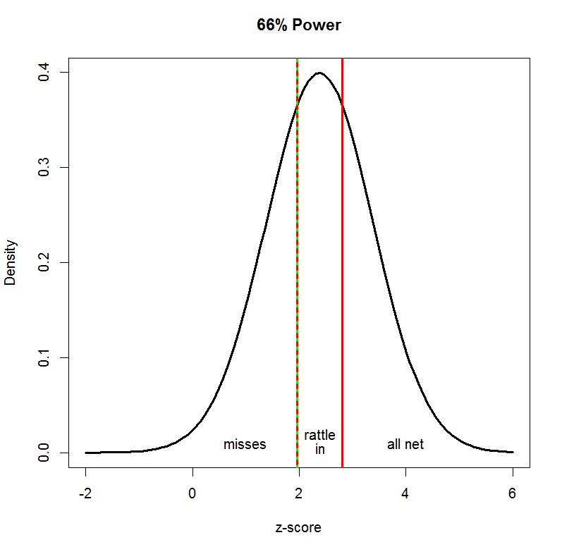
For a pair of exact replication studies, this means that there is only a 10% chance (32% * 32%) to get two rattle-in successes in a row. In contrast, there is a 90% chance that misses were not reported or that an honest report of successful studies would have produced at least one all-net result (z > 2.8, p < .005).
Example: Unconscious Priming Influences Behavior
I used this test to examine a famous and controversial set of exact replication studies. In Bargh, Chen, and Burrows (1996), Dr. Bargh reported two exact replication studies (studies 2a and 2b) that showed an effect of a subtle priming manipulation on behavior. Undergraduate students were primed with words that are stereotypically associated with old age. The researchers then measured the walking speed of primed participants (n = 15) and participants in a control group (n = 15).
The two studies were not only exact replications of each other; they also produced very similar results. Most readers probably expected this outcome because similar studies should produce similar results, but this false belief ignores the influence of random factors that are not under the control of a researcher. We do not expect lotto winners to win the lottery again because it is an entirely random and unlikely event. Experiments are different because there could be a systematic effect that makes a replication more likely, but in studies with low power results should not replicate exactly because random sampling error influences results.
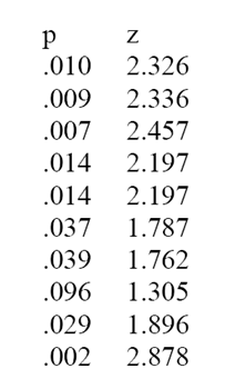
Study 1: t(28) = 2.86, p = .008 (two-tailed), z = 2.66, observed power = 76%
Study 2: t(28) = 2.16, p = .039 (two-tailed), z = 2.06, observed power = 54%
The median power of these two studies is 65%. However, even if median power were lower or higher, the maximum probability of obtaining two p-values in the range between .050 and .005 remains just 10%.
Although this study has been cited over 1,000 times, replication studies are rare.
One of the few published replication studies was reported by Cesario, Plaks, and Higgins (2006). Naïve readers might take the significant results in this replication study as evidence that the effect is real. However, this study produced yet another lucky success.
Study 3: t(62) = 2.41, p = .019, z = 2.35, observed power = 65%.
The chances of obtaining three lucky successes in a row is only 3% (32% *32% * 32*). Moreover, with a median power of 65% and a reported success rate of 100%, the success rate is inflated by 35%. This suggests that the true power of the reported studies is considerably lower than the observed power of 65% and that observed power is inflated because failed studies were not reported.
The R-Index corrects for inflation by subtracting the inflation rate from observed power (65% – 35%). This means the R-Index for this set of published studies is 30%.
This R-Index can be compared to several benchmarks.
An R-Index of 22% is consistent with the null-hypothesis being true and failed attempts are not reported.
An R-Index of 40% is consistent with 30% true power and all failed attempts are not reported.
It is therefore not surprising that other researchers were not able to replicate Bargh’s original results, even though they increased statistical power by using larger samples (Pashler et al. 2011, Doyen et al., 2011).
In conclusion, it is unlikely that Dr. Bargh’s original results were the only studies that they conducted. In an interview, Dr. Bargh revealed that the studies were conducted in 1990 and 1991 and that they conducted additional studies until the publication of the two studies in 1996. Dr. Bargh did not reveal how many studies they conducted over the span of 5 years and how many of these studies failed to produce significant evidence of priming. If Dr. Bargh himself conducted studies that failed, it would not be surprising that others also failed to replicate the published results. However, in a personal email, Dr. Bargh assured me that “we did not as skeptics might presume run many studies and only reported the significant ones. We ran it once, and then ran it again (exact replication) in order to make sure it was a real effect.” With a 10% probability, it is possible that Dr. Bargh was indeed lucky to get two rattling-in findings in a row. However, his aim to demonstrate the robustness of an effect by trying to show it again in a second small study is misguided. The reason is that it is highly likely that the effect will not replicate or that the first study was already a lucky finding after some failed pilot studies. Underpowered studies cannot provide strong evidence for the presence of an effect and conducting multiple underpowered studies reduces the credibility of successes because the probability of this outcome to occur even when an effect is present decreases with each study (Schimmack, 2012). Moreover, even if Bargh was lucky to get two rattling-in results in a row, others will not be so lucky and it is likely that many other researchers tried to replicate this sensational finding, but failed to do so. Thus, publishing lucky results hurts science nearly as much as the failure to report failed studies by the original author.
Dr. Bargh also failed to realize how lucky he was to obtain his results, in his response to a published failed-replication study by Doyen. Rather than acknowledging that failures of replication are to be expected, Dr. Bargh criticized the replication study on methodological grounds. There would be a simple solution to test Dr. Bargh’s hypothesis that he is a better researcher and that his results are replicable when the study is properly conducted. He should demonstrate that he can replicate the result himself.
In an interview, Tom Bartlett asked Dr. Bargh why he didn’t conduct another replication study to demonstrate that the effect is real. Dr. Bargh’s response was that “he is aware that some critics believe he’s been pulling tricks, that he has a “special touch” when it comes to priming, a comment that sounds like a compliment but isn’t. “I don’t think anyone would believe me,” he says.” The problem for Dr. Bargh is that there is no reason to believe his original results, either. Two rattling-in results alone do not constitute evidence for an effect, especially when this result could not be replicated in an independent study. NBA players have to make free-throws in front of a large audience for a free-throw to count. If Dr. Bargh wants his findings to count, he should demonstrate his famous effect in an open replication study. To avoid embarrassment, it would be necessary to increase the power of the replication study because it is highly unlikely that even Dr. Bargh can continuously produce significant results with samples of N = 30 participants. Even if the effect is real, sampling error is simply too large to demonstrate the effect consistently. Knowledge about statistical power is power. Knowledge about post-hoc power can be used to detect incredible results. Knowledge about a priori power can be used to produce credible results.
Swish!