Category Archives: Power

“Do Studies of Statistical Power Have an Effect on the Power of Studies?” by Peter Sedlmeier and Gerg Giegerenzer

The article with the witty title “Do Studies of Statistical Power Have an Effect on the Power of Studies?” builds on Cohen’s (1962) seminal power analysis of psychological research.

The main point of the article can be summarized in one word: No. Statistical power has not increased after Cohen published his finding that statistical power is low.

One important contribution of the article was a meta-analysis of power analyses that applied Cohen’s method to a variety of different journals. The table below shows that power estimates vary by journal assuming that the effect size was medium according to Cohen’s criteria of small, medium, and large effect sizes. The studies are sorted by power estimates from the highest to the lowest value, which provides a power ranking of journals based on Cohen’s method. I also included the results of Sedlmeier and Giegerenzer’s power analysis of the 1984 volume of the Journal of Abnormal Psychology (the Journal of Social and Abnormal Psychology was split into Journal of Abnormal Psychology and Journal of Personality and Social Psychology). I used the mean power (50%) rather than median power (44%) because the mean power is consistent with the predicted success rate in the limit. In contrast, the median will underestimate the success rate in a set of studies with heterogeneous effect sizes.

JOURNAL TITLE YEAR Power%
Journal of Marketing Research 1981 89
American Sociological Review 1974 84
Journalism Quarterly, The Journal of Broadcasting 1976 76
American Journal of Educational Psychology 1972 72
Journal of Research in Teaching 1972 71
Journal of Applied Psychology 1976 67
Journal of Communication 1973 56
The Research Quarterly 1972 52
Journal of Abnormal Psychology 1984 50
Journal of Abnormal and Social Psychology 1962 48
American Speech and Hearing Research & Journal of Communication Disorders 1975 44
Counseler Education and Supervision 1973 37


The table shows that there is tremendous variability in power estimates for different journals ranging from as high as 89% (9 out of 10 studies will produce a significant result when an effect is present) to the lowest estimate of  37% power (only 1 out of 3 studies will produce a significant result when an effect is present).

The table also shows that the Journal of Abnormal and Social Psychology and its successor the Journal of Abnormal Psychology yielded nearly identical power estimates. This finding is the key finding that provides empirical support for the claim that power in the Journal of Abnormal Psychology has not increased over time.

The average power estimate for all journals in the table is 62% (median 61%).  The list of journals is not a representative set of journals and few journals are core psychology journals. Thus, the average power may be different if a representative set of journals had been used.

The average for the three core psychology journals (JASP & JAbnPsy,  JAP, AJEduPsy) is 67% (median = 63%) is slightly higher. The latter estimate is likely to be closer to the typical power in psychology in general rather than the prominently featured estimates based on the Journal of Abnormal Psychology. Power could be lower in this journal because it is more difficult to recruit patients with a specific disorder than participants from undergraduate classes. However, only more rigorous studies of power for a broader range of journals and more years can provide more conclusive answers about the typical power of a single statistical test in a psychology journal.

The article also contains some important theoretical discussions about the importance of power in psychological research. One important issue concerns the treatment of multiple comparisons. For example, a multi-factorial design produces an exponential number of statistical comparisons. With two conditions, there is only one comparison. With three conditions, there are three comparisons (C1 vs. C2, C1 vs. C3, and C2 vs. C3). With 5 conditions, there are 10 comparisons. Standard statistical methods often correct for these multiple comparisons. One consequence of this correction for multiple comparisons is that the power of each statistical test decreases. An effect that would be significant in a simple comparison of two conditions would not be significant if this test is part of a series of tests.

Sedlmeier and Giegerenzer used the standard criterion of p < .05 (two-tailed) for their main power analysis and for the comparison with Cohen’s results. However, many articles presented results using a more stringent criterion of significance. If the criterion used by authors would have been used for the power analysis, power decreased further. About 50% of all articles used an adjusted criterion value and if the adjusted criterion value was used power was only 37%.

Sedlmeier and Giegerenzer also found another remarkable difference between articles in 1960 and in 1984. Most articles in 1960 reported the results of a single study. In 1984 many articles reported results from two or more studies. Sedlmeier and Giegerenzer do not discuss the statistical implications of this change in publication practices. Schimmack (2012) introduced the concept of total power to highlight the problem of publishing articles that contain multiple studies with modest power. If studies are used to provide empirical support for an effect, studies have to show a significant effect. For example, Study 1 shows an effect with female participants. Study 2 examines whether the effect can also be demonstrated with male participants. If Study 2 produces a non-significant result, it is not clear how this finding should be interpreted. It may show that the effect does not exist for men. It may show that the first result was just a fluke finding due to sampling error. Or it may show that the effect exists equally for men and women but studies had only 50% power to produce a significant result. In this case, it is expected that one study will produce a significant result and one will produce a non-significant result, but in the long-run significant results are equally likely with male or female participants. Given the difficulty of interpreting a non-significant result, it would be important to conduct a more powerful study that examines gender differences in a more powerful study with more female and male participants. However, this is not what researchers do. Rather, multiple study articles contain only the studies that produced significant results. The rate of successful studies in psychology journals is over 90% (Sterling et al., 1995). However, this outcome is extremely likely in multiple studies where studies have only 50% power to get a significant result in a single attempt. For each additional attempt, the probability to obtain only significant results decreases exponentially (1 Study, 50%, 2 Studies 25%, 3 Studies 12.5%, 4 Studies 6.75%).

The fact that researchers only publish studies that worked is well-known in the research community. Many researchers believe that this is an acceptable scientific practice. However, consumers of scientific research may have a different opinion about this practice. Publishing only studies that produced the desired outcome is akin to a fund manager that only publishes the return rate of funds that gained money and excludes funds with losses. Would you trust this manager to take care of your retirement? It is also akin to a gambler that only remembers winnings. Would you marry a gambler who believes that gambling is ok because you can earn money that way?

I personally do not trust obviously biased information. So, when researchers present 5 studies with significant results, I wonder whether they really had the statistical power to produce these results or whether they simply did not publish results that failed to confirm their claims. To answer this question it is essential to estimate the actual power of individual studies to produce significant results; that is, it is necessary to estimate the typical power in this field, of this researcher, or in the journal that published the results.

In conclusion, Sedlmeier and Gigerenzer made an important contribution to the literature by providing the first power-ranking of scientific journals and the first temporal analyses of time trends in power. Although they probably hoped that their scientific study of power would lead to an increase in statistical power, the general consensus is that their article failed to change scientific practices in psychology. In fact, some journals required more and more studies as evidence for an effect (some articles contain 9 studies) without any indication that researchers increased power to ensure that their studies could actually provide significant results for their hypotheses. Moreover, the topic of statistical power remained neglected in the training of future psychologists.

I recommend Sedlmeier and Gigerenzer’s article as essential reading for anybody interested in improving the credibility of psychology as a rigorous empirical science.

As always, comments (positive or negative) are always welcome.

Distinguishing Questionable Research Practices from Publication Bias

It is well-known that scientific journals favor statistically significant results (Sterling, 1959). This phenomenon is known as publication bias. Publication bias can be easily detected by comparing the observed statistical power of studies with the success rate in journals. Success rates of 90% or more would only be expected if most theoretical predictions are true and empirical studies have over 90% statistical power to produce significant results. Estimates of statistical power range from 20% to 50% (Button et al., 2015, Cohen, 1962). It follows that for every published significant result an unknown number of non-significant results has occurred that remained unpublished. These results linger in researchers proverbial file-drawer or more literally in unpublished data sets on researchers’ computers.

The selection of significant results also creates an incentive for researchers to produce significant results. In rare cases, researchers simply fabricate data to produce significant results. However, scientific fraud is rare. A more serious threat to the integrity of science is the use of questionable research practices. Questionable research practices are all research activities that create a systematic bias in empirical results. Although systematic bias can produce too many or too few significant results, the incentive to publish significant results suggests that questionable research practices are typically used to produce significant results.

In sum, publication bias and questionable research practices contribute to an inflated success rate in scientific journals. So far, it has been difficult to examine the prevalence of questionable research practices in science. One reason is that publication bias and questionable research practices are conceptually overlapping. For example, a research article may report the results of a 2 x 2 x 2 ANOVA or a regression analysis with 5 predictor variables. The article may only report the significant results and omit detailed reporting of the non-significant results. For example, researchers may state that none of the gender effects were significant and not report the results for main effects or interaction with gender. I classify these cases as publication bias because each result tests a different hypothesis., even if the statistical tests are not independent.

Questionable research practices are practices that change the probability of obtaining a specific significant result. An example would be a study with multiple outcome measures that would support the same theoretical hypothesis. For example, a clinical trial of an anti-depressant might include several depression measures. In this case, a researcher can increase the chances of a significant result by conducting tests for each measure. Other questionable research practices would be optional stopping once a significant result is obtained, selective deletion of cases based on the results after deletion. A common consequence of these questionable practices is that they will produce results that meet the significance criterion, but deviate from the distribution that is expected simply on the basis of random sampling error.

A number of articles have tried to examine the prevalence of questionable research practices by comparing the frequency of p-values above and below the typical criterion of statistical significance, namely a p-value less than .05. The logic is that random error would produce a nearly equal amount of p-values just above .05 (e.g., p = .06) and below .05 (e.g., p = .04). According to this logic, questionable research practices are present, if there are more p-values just below the criterion than p-values just above the criterion (Masicampo & Lalande, 2012).

Daniel Lakens has pointed out some problems with this approach. The most crucial problem is that publication bias alone is sufficient to predict a lower frequency of p-values below the significance criterion. After all, these p-values imply a non-significant result and non-significant results are subject to publication bias. The only reason why p-values of .06 are reported with higher frequency than p-values of .11 is that p-values between .05 and .10 are sometimes reported as marginally significant evidence for a hypothesis. Another problem is that many p-values of .04 are not reported as p = .04, but are reported as p < .05. Thus, the distribution of p-values close to the criterion value provides unreliable information about the prevalence of questionable research practices.

In this blog post, I introduce an alternative approach to the detection of questionable research practices that produce just significant results. Questionable research practices and publication bias have different effects on the distribution of p-values (or corresponding measures of strength of evidence). Whereas publication bias will produce a distribution that is consistent with the average power of studies, questionable research practice will produce an abnormal distribution with a peak just below the significance criterion. In other words, questionable research practices produce a distribution with too few non-significant results and too few highly significant results.

I illustrate this test of questionable research practices with post-hoc-power analysis of three journals. One journal shows neither signs of publication bias, nor significant signs of questionable research practices. The second journal shows clear evidence of publication bias, but no evidence of questionable research practices. The third journal illustrates the influence of publication bias and questionable research practices.

Example 1: A Relatively Unbiased Z-Curve

The first example is based on results published during the years 2010-2014 in the Journal of Experimental Psychology: Learning, Memory, and Cognition. A text-mining program searched all articles for publications of F-tests, t-tests, correlation coefficients, regression coefficients, odds-ratios, confidence intervals, and z-tests. Due to the inconsistent and imprecise reporting of p-values (p = .02 or p < .05), p-values were not used. All statistical tests were converted into absolute z-scores.

The program found 14,800 tests. 8,423 tests were in the critical interval between z = 2 and z = 6 that is used for estimation of 4 non-centrality parameters and 4 weights that are used to model the distribution of z-values between 2 and 6 and to estimate the distribution in the range from 0 to 2. Z-values greater than 6 are not used because they correspond to Power close to 1. 11% of all tests fall into this region of z-scores that are not shown.

PHP-Curve JEP-LMCThe histogram and the blue density distribution show the observed data. The green curve shows the predicted distribution based on the post-hoc power analysis. Post-hoc power analysis suggests that the average power of significant results is 67%. Power for all statistical tests is estimated to be 58% (including 11% of z-scores greater than 6, power is .58*.89 + .11 = 63%). More important is the predicted distribution of z-scores. The predicted distribution on the left side of the criterion value matches the observed distribution rather well. This shows that there are not a lot of missing non-significant results. In other words, there does not appear to be a file-drawer of studies with non-significant results. There is also only a very small blip in the observed data just at the level of statistical significance. The close match between the observed and predicted distributions suggests that results in this journal are relatively free of systematic bias due to publication bias or questionable research practices.

Example 2: A Z-Curve with Publication Bias

The second example is based on results published in the Attitudes & Social Cognition Section of the Journal of Personality and Social Psychology. The text-mining program retrieved 5,919 tests from articles published between 2010 and 2014. 3,584 tests provided z-scores in the range from 2 to 6 that is being used for model fitting.

PHP-Curve JPSP-ASC

The average power of significant results in JPSP-ASC is 55%. This is significantly less than the average power in JEP-LMC, which was used for the first example. The estimated power for all statistical tests, including those in the estimated file drawer, is 35%. More important is the estimated distribution of z-values. On the right side of the significance criterion the estimated curve shows relatively close fit to the observed distribution. This finding shows that random sampling error alone is sufficient to explain the observed distribution. However, on the left side of the distribution, the observed z-scores drop off steeply. This drop is consistent with the effect of publication bias that researchers do not report all non-significant results. There is only a slight hint that questionable research practices are also present because observed z-scores just above the criterion value are a bit more frequent than the model predicts. However, this discrepancy is not conclusive because the model could increase the file drawer, which would produce a steeper slope. The most important characteristic of this z-curve is the steep cliff on the left side of the criterion value and the gentle slope on the right side of the criterion value.

Example 3: A Z-Curve with Questionable Research Practices.

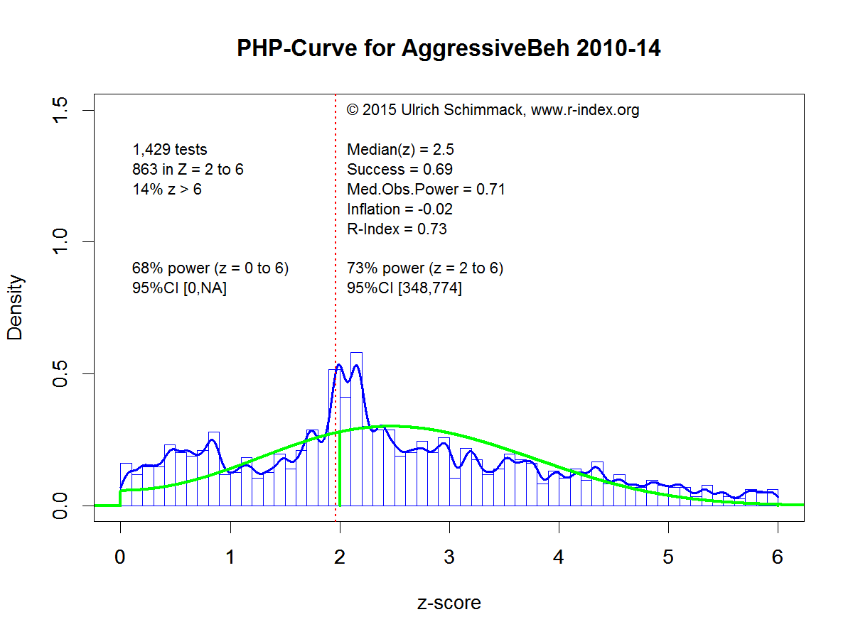
Example 3 uses results published in the journal Aggressive Behavior during the years 2010 to 2014. The text mining program found 1,429 results and 863 z-scores in the range from 2 to 6 that were used for the post-hoc-power analysis.

PHP-Curve for AggressiveBeh 2010-14


The average power for significant results in the range from 2 to 6 is 73%, which is similar to the power estimate in the first example. The power estimate that includes non-significant results is 68%. The power estimate is similar because there is no evidence of a file drawer with many underpowered studies. In fact, there are more observed non-significant results than predicted non-significant results, especially for z-scores close to zero. This outcome shows some problems of estimating the frequency of non-significant results based on the distribution of significant results. More important, the graph shows a cluster of z-scores just above and below the significance criterion. The step cliff to the left of the criterion might suggest publication bias, but the whole distribution does not show evidence of publication bias. Moreover, the steep cliff on the right side of the cluster cannot be explained with publication bias. Only questionable research practices can produce this cliff because publication bias relies on random sampling error which leads to a gentle slope of z-scores as shown in the second example.

Prevalence of Questionable Research Practices

The examples suggest that the distribution of z-scores can be used to distinguish publication bias and questionable research practices. Based on this approach, the prevalence of questionable research practices would be rare. The journal Aggressive Behavior is exceptional. Most journals show a pattern similar to Example 2, with varying sizes of the file drawer. However, this does not mean that questionable research practices are rare because it is most likely that the pattern observed in Example 2 is a combination of questionable research practices and publication bias. As shown in Example 2, the typical power of statistical tests that produce a significant result is about 60%. However, researchers do not know which experiments will produce significant results. Slight modifications in experimental procedures, so-called hidden moderators, can easily change an experiment with 60% power into an experiment with 30% power. Thus, the probability of obtaining a significant result in a replication study is less than the nominal power of 60% that is implied by post-hoc-power analysis. With only 30% to 60% power, researchers will frequently encounter results that fail to produce an expected significant result. In this case, researchers have two choices to avoid reporting a non-significant result. They can put the study in the file-drawer or they can try to salvage the study with the help of questionable research practices. It is likely that researchers will do both and that the course of action depends on the results. If the data show a trend in the right direction, questionable research practices seem an attractive alternative. If the data show a trend in the opposite direction, it is more likely that the study will be terminated and the results remain unreported.

Simons et al. (2011) conducted some simulation studies and found that even extreme use of multiple questionable research practices (p-hacking) will produce a significant result in at most 60% of cases, when the null-hypothesis is true. If such extreme use of questionable research practices were widespread, z-curve would produce corrected power estimates well-below 50%. There is no evidence that extreme use of questionable research practices is prevalent. In contrast, there is strong evidence that researchers conduct many more studies than they actually report and that many of these studies have a low probability of success.

Implications of File-Drawers for Science

First, it is clear that researchers could be more effective if they would use existing resources more effectively. An fMRI study with 20 participants costs about $10,000. Conducting a study that costs $10,000 that has only a 50% probability of producing a significant result is wasteful and should not be funded by taxpayers. Just publishing the non-significant result does not fix this problem because a non-significant result in a study with 50% power is inconclusive. Even if the predicted effect exists, one would expect a non-significant result in ever second study.   Instead of wasting $10,000 on studies with 50% power, researchers should invest $20,000 in studies with higher power (unfortunately, power does not increase proportional to resources). With the same research budget, more money would contribute to results that are being published. Thus, without spending more money, science could progress faster.

Second, higher powered studies make non-significant results more relevant. If a study had 80% power, there is only a 20% chance to get a non-significant result if an effect is present. If a study had 95% power, the chance of a non-significant result would be just as low as the chance of a false positive result. In this case, it is noteworthy that a theoretical prediction was not confirmed. In a set of high-powered studies, a post-hoc power analysis would show a bimodal distribution with clusters of z-scores around 0 for true null-hypothesis and a cluster of z-scores of 3 or higher for clear effects. Type-I and Type-II errors would be rare.

Third, Example 3 shows that the use of questionable research practices becomes detectable in the absence of a file drawer and that it would be harder to publish results that were obtained with questionable research practices.

Finally, the ability to estimate the size of file-drawers may encourage researchers to plan studies more carefully and to invest more resources into studies to keep their file drawers small because a large file-drawer may harm reputation or decrease funding.

In conclusion, post-hoc power analysis of large sets of data can be used to estimate the size of the file drawer based on the distribution of z-scores on the right side of a significance criterion. As file-drawers harm science, this tool can be used as an incentive to conduct studies that produce credible results and thus reducing the need for dishonest research practices. In this regard, the use of post-hoc power analysis complements other efforts towards open science such as preregistration and data sharing.

REPLICABILITY RANKING OF 26 PSYCHOLOGY JOURNALS

THEORETICAL BACKGROUND

Neyman & Pearson (1933) developed the theory of type-I and type-II errors in statistical hypothesis testing.

A type-I error is defined as the probability of rejecting the null-hypothesis (i.e., the effect size is zero) when the null-hypothesis is true.

A type-II error is defined as the probability of failing to reject the null-hypothesis when the null-hypothesis is false (i.e., there is an effect).

A common application of statistics is to provide empirical evidence for a theoretically predicted relationship between two variables (cause-effect or covariation). The results of an empirical study can produce two outcomes. Either the result is statistically significant or it is not statistically significant. Statistically significant results are interpreted as support for a theoretically predicted effect.

Statistically non-significant results are difficult to interpret because the prediction may be false (the null-hypothesis is true) or a type-II error occurred (the theoretical prediction is correct, but the results fail to provide sufficient evidence for it).

To avoid type-II errors, researchers can design studies that reduce the type-II error probability. The probability of avoiding a type-II error when a predicted effect exists is called power. It could also be called the probability of success because a significant result can be used to provide empirical support for a hypothesis.

Ideally researchers would want to maximize power to avoid type-II errors. However, powerful studies require more resources. Thus, researchers face a trade-off between the allocation of resources and their probability to obtain a statistically significant result.

Jacob Cohen dedicated a large portion of his career to help researchers with the task of planning studies that can produce a successful result, if the theoretical prediction is true. He suggested that researchers should plan studies to have 80% power. With 80% power, the type-II error rate is still 20%, which means that 1 out of 5 studies in which a theoretical prediction is true would fail to produce a statistically significant result.

Cohen (1962) examined the typical effect sizes in psychology and found that the typical effect size for the mean difference between two groups (e.g., men and women or experimental vs. control group) is about half-of a standard deviation. The standardized effect size measure is called Cohen’s d in his honor. Based on his review of the literature, Cohen suggested that an effect size of d = .2 is small, d = .5 moderate, and d = .8. Importantly, a statistically small effect size can have huge practical importance. Thus, these labels should not be used to make claims about the practical importance of effects. The main purpose of these labels is that researchers can better plan their studies. If researchers expect a large effect (d = .8), they need a relatively small sample to have high power. If researchers expect a small effect (d = .2), they need a large sample to have high power.   Cohen (1992) provided information about effect sizes and sample sizes for different statistical tests (chi-square, correlation, ANOVA, etc.).

Cohen (1962) conducted a meta-analysis of studies published in a prominent psychology journal. Based on the typical effect size and sample size in these studies, Cohen estimated that the average power in studies is about 60%. Importantly, this also means that the typical power to detect small effects is less than 60%. Thus, many studies in psychology have low power and a high type-II error probability. As a result, one would expect that journals often report that studies failed to support theoretical predictions. However, the success rate in psychological journals is over 90% (Sterling, 1959; Sterling, Rosenbaum, & Weinkam, 1995). There are two explanations for discrepancies between the reported success rate and the success probability (power) in psychology. One explanation is that researchers conduct multiple studies and only report successful studies. The other studies remain unreported in a proverbial file-drawer (Rosenthal, 1979). The other explanation is that researchers use questionable research practices to produce significant results in a study (John, Loewenstein, & Prelec, 2012). Both practices have undesirable consequences for the credibility and replicability of published results in psychological journals.

A simple solution to the problem would be to increase the statistical power of studies. If the power of psychological studies in psychology were over 90%, a success rate of 90% would be justified by the actual probability of obtaining significant results. However, meta-analysis and method articles have repeatedly pointed out that psychologists do not consider statistical power in the planning of their studies and that studies continue to be underpowered (Maxwell, 2004; Schimmack, 2012; Sedlmeier & Giegerenzer, 1989).

One reason for the persistent neglect of power could be that researchers have no awareness of the typical power of their studies. This could happen because observed power in a single study is an imperfect indicator of true power (Yuan & Maxwell, 2005). If a study produced a significant result, the observed power is at least 50%, even if the true power is only 30%. Even if the null-hypothesis is true, and researchers publish only type-I errors, observed power is dramatically inflated to 62%, when the true power is only 5% (the type-I error rate). Thus, Cohen’s estimate of 60% power is not very reassuring.

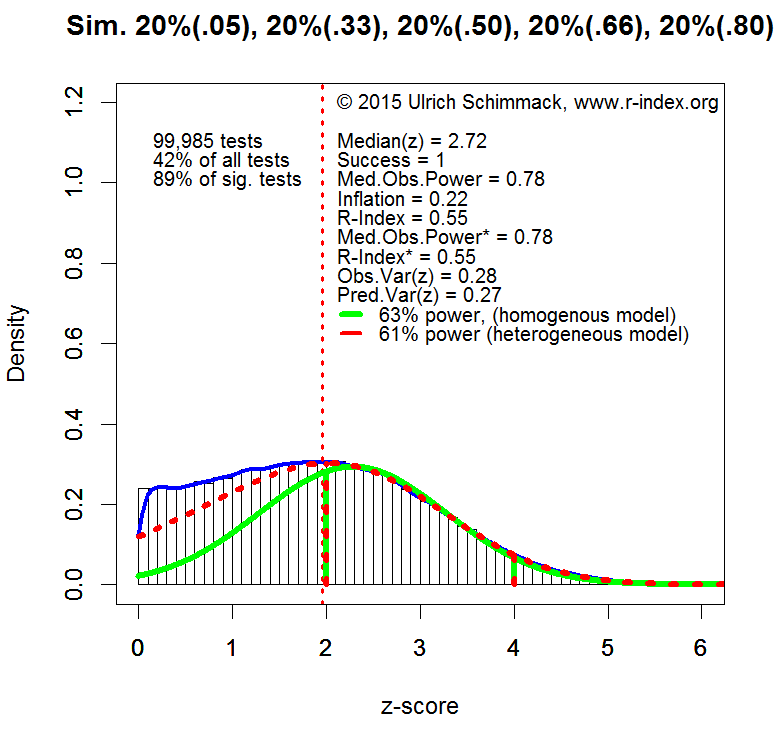
Over the past years, Schimmack and Brunner have developed a method to estimate power for sets of studies with heterogeneous designs, sample sizes, and effect sizes. A technical report is in preparation. The basic logic of this approach is to convert results of all statistical tests into z-scores using the one-tailed p-value of a statistical test.  The z-scores provide a common metric for observed statistical results. The standard normal distribution predicts the distribution of observed z-scores for a fixed value of true power.   However, for heterogeneous sets of studies the distribution of z-scores is a mixture of standard normal distributions with different weights attached to various power values. To illustrate this method, the histograms of z-scores below show simulated data with 10,000 observations with varying levels of true power: 20% null-hypotheses being true (5% power), 20% of studies with 33% power, 20% of studies with 50% power, 20% of studies with 66% power, and 20% of studies with 80% power.

RepRankSimulation

The plot shows the distribution of absolute z-scores (there are no negative effect sizes). The plot is limited to z-scores below 6 (N = 99,985 out of 10,000). Z-scores above 6 standard deviations from zero are extremely unlikely to occur by chance. Even with a conservative estimate of effect size (lower bound of 95% confidence interval), observed power is well above 99%. Moreover, quantum physics uses Z = 5 as a criterion to claim success (e.g., discovery of Higgs-Boson Particle). Thus, Z-scores above 6 can be expected to be highly replicable effects.

Z-scores below 1.96 (the vertical dotted red line) are not significant for the standard criterion of (p < .05, two-tailed). These values are excluded from the calculation of power because these results are either not reported or not interpreted as evidence for an effect. It is still important to realize that true power of all experiments would be lower if these studies were included because many of the non-significant results are produced by studies with 33% power. These non-significant results create two problems. Researchers wasted resources on studies with inconclusive results and readers may be tempted to misinterpret these results as evidence that an effect does not exist (e.g., a drug does not have side effects) when an effect is actually present. In practice, it is difficult to estimate power for non-significant results because the size of the file-drawer is difficult to estimate.

It is possible to estimate power for any range of z-scores, but I prefer the range of z-scores from 2 (just significant) to 4. A z-score of 4 has a 95% confidence interval that ranges from 2 to 6. Thus, even if the observed effect size is inflated, there is still a high chance that a replication study would produce a significant result (Z > 2). Thus, all z-scores greater than 4 can be treated as cases with 100% power. The plot also shows that conclusions are unlikely to change by using a wider range of z-scores because most of the significant results correspond to z-scores between 2 and 4 (89%).

The typical power of studies is estimated based on the distribution of z-scores between 2 and 4. A steep decrease from left to right suggests low power. A steep increase suggests high power. If the peak (mode) of the distribution were centered over Z = 2.8, the data would conform to Cohen’s recommendation to have 80% power.

Using the known distribution of power to estimate power in the critical range gives a power estimate of 61%. A simpler model that assumes a fixed power value for all studies produces a slightly inflated estimate of 63%. Although the heterogeneous model is correct, the plot shows that the homogeneous model provides a reasonable approximation when estimates are limited to a narrow range of Z-scores. Thus, I used the homogeneous model to estimate the typical power of significant results reported in psychological journals.

DATA

The results presented below are based on an ongoing project that examines power in psychological journals (see results section for the list of journals included so far). The set of journals does not include journals that primarily publish reviews and meta-analysis or clinical and applied journals. The data analysis is limited to the years from 2009 to 2015 to provide information about the typical power in contemporary research. Results regarding historic trends will be reported in a forthcoming article.

I downloaded pdf files of all articles published in the selected journals and converted the pdf files to text files. I then extracted all t-tests and F-tests that were reported in the text of the results section searching for t(df) or F(df1,df2). All t and F statistics were converted into one-tailed p-values and then converted into z-scores.

RepRankAll

The plot above shows the results based on 218,698 t and F tests reported between 2009 and 2015 in the selected psychology journals. Unlike the simulated data, the plot shows a steep drop for z-scores just below the threshold of significance (z = 1.96). This drop is due to the tendency not to publish or report non-significant results. The heterogeneous model uses the distribution of non-significant results to estimate the size of the file-drawer (unpublished non-significant results). However, for the present purpose the size of the file-drawer is irrelevant because power is estimated only for significant results for Z-scores between 2 and 4.

The green line shows the best fitting estimate for the homogeneous model. The red curve shows fit of the heterogeneous model. The heterogeneous model is doing a much better job at fitting the long tail of highly significant results, but for the critical interval of z-scores between 2 and 4, the two models provide similar estimates of power (55% homogeneous & 53% heterogeneous model).   If the range is extended to z-scores between 2 and 6, power estimates diverge (82% homogenous, 61% heterogeneous). The plot indicates that the heterogeneous model fits the data better and that the 61% estimate is a better estimate of true power for significant results in this range. Thus, the results are in line with Cohen (1962) estimate that psychological studies average 60% power.

REPLICABILITY RANKING

The distribution of z-scores between 2 and 4 was used to estimate the average power separately for each journal. As power is the probability to obtain a significant result, this measure estimates the replicability of results published in a particular journal if researchers would reproduce the studies under identical conditions with the same sample size (exact replication). Thus, even though the selection criterion ensured that all tests produced a significant result (100% success rate), the replication rate is expected to be only about 50%, even if the replication studies successfully reproduce the conditions of the published studies. The table below shows the replicability ranking of the journals, the replicability score, and a grade. Journals are graded based on a scheme that is similar to grading schemes for undergraduate students (below 50 = F, 50-59 = E, 60-69 = D, 70-79 = C, 80-89 = B, 90+ = A).

ReplicabilityRanking

The average value in 2000-2014 is 57 (D+). The average value in 2015 is 58 (D+). The correlation for the values in 2010-2014 and those in 2015 is r = .66.   These findings show that the replicability scores are reliable and that journals differ systematically in the power of published studies.

LIMITATIONS

The main limitation of the method is that focuses on t and F-tests. The results might change when other statistics are included in the analysis. The next goal is to incorporate correlations and regression coefficients.

The second limitation is that the analysis does not discriminate between primary hypothesis tests and secondary analyses. For example, an article may find a significant main effect for gender, but the critical test is whether gender interacts with an experimental manipulation. It is possible that some journals have lower scores because they report more secondary analyses with lower power. To address this issue, it will be necessary to code articles in terms of the importance of statistical test.

The ranking for 2015 is based on the currently available data and may change when more data become available. Readers should also avoid interpreting small differences in replicability scores as these scores are likely to fluctuate. However, the strong correlation over time suggests that there are meaningful differences in the replicability and credibility of published results across journals.

CONCLUSION

This article provides objective information about the replicability of published findings in psychology journals. None of the journals reaches Cohen’s recommended level of 80% replicability. Average replicability is just about 50%. This finding is largely consistent with Cohen’s analysis of power over 50 years ago. The publication of the first replicability analysis by journal should provide an incentive to editors to increase the reputation of their journal by paying more attention to the quality of the published data. In this regard, it is noteworthy that replicability scores diverge from traditional indicators of journal prestige such as impact factors. Ideally, the impact of an empirical article should be aligned with the replicability of the empirical results. Thus, the replicability index may also help researchers to base their own research on credible results that are published in journals with a high replicability score and to avoid incredible results that are published in journals with a low replicability score. Ultimately, I can only hope that journals will start competing with each other for a top spot in the replicability rankings and as a by-product increase the replicability of published findings and the credibility of psychological science.

When Exact Replications Are Too Exact: The Lucky-Bounce-Test for Pairs of Exact Replication Studies

Imagine an NBA player has an 80% chance to make one free throw. What is the chance that he makes both free throws? The correct answer is 64% (80% * 80%).

Now consider the possibility that it is possible to distinguish between two types of free throws. Some free throws are good; they don’t touch the rim and make a swishing sound when they go through the net (all net). The other free throws bounce of the rim and go in (rattling in).

What is the probability that an NBA player with an 80% free throw percentage makes a free throw that is all net or rattles in? It is more likely that an NBA player with an 80% free throw average makes a perfect free throw because a free throw that rattles in could easily have bounded the wrong way, which would lower the free throw percentage. To achieve an 80% free throw percentage, most free throws have to be close to perfect.

Let’s say the probability of hitting the rim and going in is 30%. With an 80% free throw average, this means that the majority of free throws are in the close-to-perfect category (20% misses, 30% rattle-in, 50% close-to-perfect).

What does this have to do with science? A lot!

The reason is that the outcome of a scientific study is a bit like throwing free throws. One factor that contributes to a successful study is skill (making correct predictions, avoiding experimenter errors, and conducting studies with high statistical power). However, another factor is random (a lucky or unlucky bounce).

The concept of statistical power is similar to an NBA players’ free throw percentage. A researcher who conducts studies with 80% statistical power is going to have an 80% success rate (that is, if all predictions are correct). In the remaining 20% of studies, a study will not produce a statistically significant result, which is equivalent to missing a free throw and not getting a point.

Many years ago, Jacob Cohen observed that researchers often conduct studies with relatively low power to produce a statistically significant result. Let’s just assume right now that a researcher conducts studies with 60% power. This means, researchers would be like NBA players with a 60% free-throw average.

Now imagine that researchers have to demonstrate an effect not only once, but also a second time in an exact replication study. That is researchers have to make two free throws in a row. With 60% power, the probability to get two significant results in a row is only 36% (60% * 60%). Moreover, many of the freethrows that are made rattle in rather than being all net. The percentages are about 40% misses, 30% rattling in and 30% all net.

One major difference between NBA players and scientists is that NBA players have to demonstrate their abilities in front of large crowds and TV cameras, whereas scientists conduct their studies in private.

Imagine an NBA player could just go into a private room, throw two free throws and then report back how many free throws he made and the outcome of these free throws determine who wins game 7 in the playoff finals. Would you trust the player to tell the truth?

If you would not trust the NBA player, why would you trust scientists to report failed studies? You should not.

It can be demonstrated statistically that scientists are reporting more successes than the power of their studies would justify (Sterling et al., 1995; Schimmack, 2012). Amongst scientists this fact is well known, but the general public may not fully appreciate the fact that a pair of exact replication studies with significant results is often just a selection of studies that included failed studies that were not reported.

Fortunately, it is possible to use statistics to examine whether the results of a pair of studies are likely to be honest or whether failed studies were excluded. The reason is that an amateur is not only more likely to miss a free throw. An amateur is also less likely to make a perfect free throw.

Based on the theory of statistical power developed by Nyman and Pearson and popularized by Jacob Cohen, it is possible to make predictions about the relative frequency of p-values in the non-significant (failure), just significant (rattling in), and highly significant (all net) ranges.

As for made-free-throws, the distinction between lucky and clear successes is somewhat arbitrary because power is continuous. A study with a p-value of .0499 is very lucky because p = .501 would have been not significant (rattled in after three bounces on the rim). A study with p = .000001 is a clear success. Lower p-values are better, but where to draw the line?

As it turns out, Jacob Cohen’s recommendation to conduct studies with 80% power provides a useful criterion to distinguish lucky outcomes and clear successes.

Imagine a scientist conducts studies with 80% power. The distribution of observed test-statistics (e.g. z-scores) shows that this researcher has a 20% chance to get a non-significant result, a 30% chance to get a lucky significant result (p-value between .050 and .005), and a 50% chance to get a clear significant result (p < .005). If the 20% failed studies are hidden, the percentage of results that rattled in versus studies with all-net results are 37 vs. 63%. However, if true power is just 20% (an amateur), 80% of studies fail, 15% rattle in, and 5% are clear successes. If the 80% failed studies are hidden, only 25% of the successful studies are all-net and 75% rattle in.

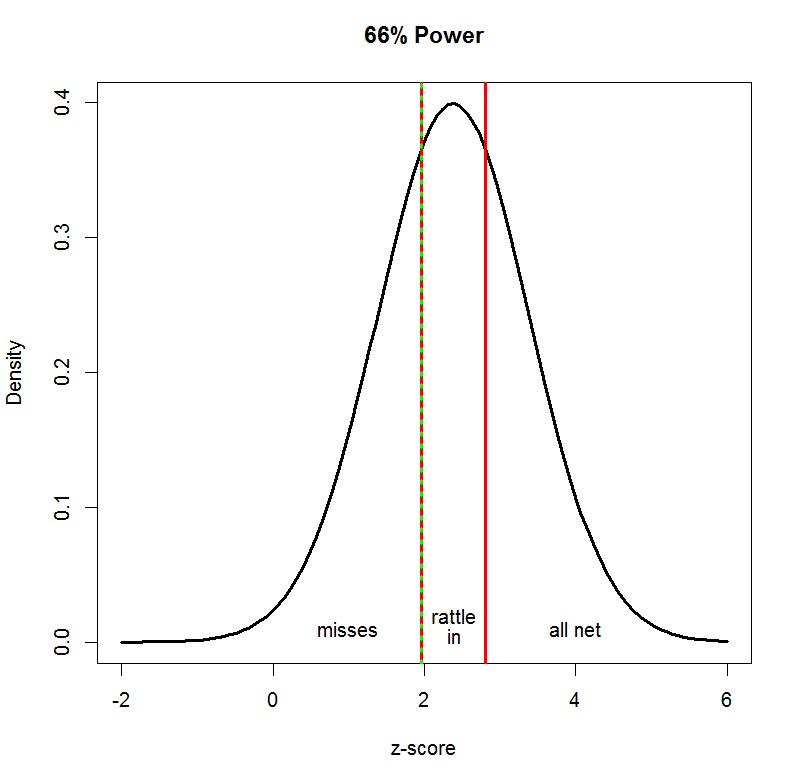
One problem with using this test to draw conclusions about the outcome of a pair of exact replication studies is that true power is unknown. To avoid this problem, it is possible to compute the maximum probability of a rattling-in result. As it turns out, the optimal true power to maximize the percentage of lucky outcomes is 66% power. With true power of 66%, one would expect 34% misses (p > .05), 32% lucky successes (.050 < p < .005), and 34% clear successes (p < .005).

LuckyBounceTest

For a pair of exact replication studies, this means that there is only a 10% chance (32% * 32%) to get two rattle-in successes in a row. In contrast, there is a 90% chance that misses were not reported or that an honest report of successful studies would have produced at least one all-net result (z > 2.8, p < .005).

Example: Unconscious Priming Influences Behavior

I used this test to examine a famous and controversial set of exact replication studies. In Bargh, Chen, and Burrows (1996), Dr. Bargh reported two exact replication studies (studies 2a and 2b) that showed an effect of a subtle priming manipulation on behavior. Undergraduate students were primed with words that are stereotypically associated with old age. The researchers then measured the walking speed of primed participants (n = 15) and participants in a control group (n = 15).

The two studies were not only exact replications of each other; they also produced very similar results. Most readers probably expected this outcome because similar studies should produce similar results, but this false belief ignores the influence of random factors that are not under the control of a researcher. We do not expect lotto winners to win the lottery again because it is an entirely random and unlikely event. Experiments are different because there could be a systematic effect that makes a replication more likely, but in studies with low power results should not replicate exactly because random sampling error influences results.

Study 1: t(28) = 2.86, p = .008 (two-tailed), z = 2.66, observed power = 76%
Study 2: t(28) = 2.16, p = .039 (two-tailed), z = 2.06, observed power = 54%

The median power of these two studies is 65%. However, even if median power were lower or higher, the maximum probability of obtaining two p-values in the range between .050 and .005 remains just 10%.

Although this study has been cited over 1,000 times, replication studies are rare.

One of the few published replication studies was reported by Cesario, Plaks, and Higgins (2006). Naïve readers might take the significant results in this replication study as evidence that the effect is real. However, this study produced yet another lucky success.

Study 3: t(62) = 2.41, p = .019, z = 2.35, observed power = 65%.

The chances of obtaining three lucky successes in a row is only 3% (32% *32% * 32*). Moreover, with a median power of 65% and a reported success rate of 100%, the success rate is inflated by 35%. This suggests that the true power of the reported studies is considerably lower than the observed power of 65% and that observed power is inflated because failed studies were not reported.

The R-Index corrects for inflation by subtracting the inflation rate from observed power (65% – 35%). This means the R-Index for this set of published studies is 30%.

This R-Index can be compared to several benchmarks.

An R-Index of 22% is consistent with the null-hypothesis being true and failed attempts are not reported.

An R-Index of 40% is consistent with 30% true power and all failed attempts are not reported.

It is therefore not surprising that other researchers were not able to replicate Bargh’s original results, even though they increased statistical power by using larger samples (Pashler et al. 2011, Doyen et al., 2011).

In conclusion, it is unlikely that Dr. Bargh’s original results were the only studies that they conducted. In an interview, Dr. Bargh revealed that the studies were conducted in 1990 and 1991 and that they conducted additional studies until the publication of the two studies in 1996. Dr. Bargh did not reveal how many studies they conducted over the span of 5 years and how many of these studies failed to produce significant evidence of priming. If Dr. Bargh himself conducted studies that failed, it would not be surprising that others also failed to replicate the published results. However, in a personal email, Dr. Bargh assured me that “we did not as skeptics might presume run many studies and only reported the significant ones. We ran it once, and then ran it again (exact replication) in order to make sure it was a real effect.” With a 10% probability, it is possible that Dr. Bargh was indeed lucky to get two rattling-in findings in a row. However, his aim to demonstrate the robustness of an effect by trying to show it again in a second small study is misguided. The reason is that it is highly likely that the effect will not replicate or that the first study was already a lucky finding after some failed pilot studies. Underpowered studies cannot provide strong evidence for the presence of an effect and conducting multiple underpowered studies reduces the credibility of successes because the probability of this outcome to occur even when an effect is present decreases with each study (Schimmack, 2012). Moreover, even if Bargh was lucky to get two rattling-in results in a row, others will not be so lucky and it is likely that many other researchers tried to replicate this sensational finding, but failed to do so. Thus, publishing lucky results hurts science nearly as much as the failure to report failed studies by the original author.

Dr. Bargh also failed to realize how lucky he was to obtain his results, in his response to a published failed-replication study by Doyen. Rather than acknowledging that failures of replication are to be expected, Dr. Bargh criticized the replication study on methodological grounds. There would be a simple solution to test Dr. Bargh’s hypothesis that he is a better researcher and that his results are replicable when the study is properly conducted. He should demonstrate that he can replicate the result himself.

In an interview, Tom Bartlett asked Dr. Bargh why he didn’t conduct another replication study to demonstrate that the effect is real. Dr. Bargh’s response was that “he is aware that some critics believe he’s been pulling tricks, that he has a “special touch” when it comes to priming, a comment that sounds like a compliment but isn’t. “I don’t think anyone would believe me,” he says.” The problem for Dr. Bargh is that there is no reason to believe his original results, either. Two rattling-in results alone do not constitute evidence for an effect, especially when this result could not be replicated in an independent study. NBA players have to make free-throws in front of a large audience for a free-throw to count. If Dr. Bargh wants his findings to count, he should demonstrate his famous effect in an open replication study. To avoid embarrassment, it would be necessary to increase the power of the replication study because it is highly unlikely that even Dr. Bargh can continuously produce significant results with samples of N = 30 participants. Even if the effect is real, sampling error is simply too large to demonstrate the effect consistently. Knowledge about statistical power is power. Knowledge about post-hoc power can be used to detect incredible results. Knowledge about a priori power can be used to produce credible results.

Swish!

A Critical Review of Cumming’s (2014) New Statistics: Reselling Old Statistics as New Statistics

Cumming (2014) wrote an article “The New Statistics: Why and How” that was published in the prestigious journal Psychological Science.   On his website, Cumming uses this article to promote his book “Cumming, G. (2012). Understanding The New Statistics: Effect Sizes, Confidence Intervals, and Meta-Analysis. New York: Routledge.”

The article clear states the conflict of interest. “The author declared that he earns royalties on his book (Cumming, 2012) that is referred to in this article.” Readers are therefore warned that the article may at least inadvertently give an overly positive account of the new statistics and an overly negative account of the old statistics. After all, why would anybody buy a book about new statistics when the old statistics are working just fine.

This blog post critically examines Cumming’s claim that his “new statistics” can solve endemic problems in psychological research that have created a replication crisis and that the old statistics are the cause of this crisis.

Like many other statisticians who are using the current replication crisis as an opportunity to sell their statistical approach, Cumming’s blames null-hypothesis significance testing (NHST) for the low credibility of research articles in Psychological Science (Francis, 2013).

In a nutshell, null-hypothesis significance testing entails 5 steps. First, researchers conduct a study that yields an observed effect size. Second, the sampling error of the design is estimated. Third, the ratio of the observed effect size and sampling error (signal-to-noise ratio) is computed to create a test-statistic (t, F, chi-square). The test-statistic is then used to compute the probability of obtaining the observed test-statistic or a larger one under the assumption that the true effect size in the population is zero (there is no effect or systematic relationship). The last step is to compare the test statistic to a criterion value. If the probability (p-value) is less than a criterion value (typically 5%), the null-hypothesis is rejected and it is concluded that an effect was present.

Cumming’s (2014) claims that we need a new way to analyze data because there is “renewed recognition of the severe flaws of null-hypothesis significance testing (NHST)” (p. 7). His new statistical approach has “no place for NHST” (p. 7). His advice is to “whenever possible, avoid using statistical significance or p values” (p. 8).

So what is wrong with NHST?

The first argument against NHST is that Ioannidis (2005) wrote an influential article with the eye-catching title “Why most published research findings are false” and most research articles use NHST to draw inferences from the observed results. Thus, NHST seems to be a flawed method because it produces mostly false results. The problem with this argument is that Ioannidis (2005) did not provide empirical evidence that most research findings are false, nor is this a particularly credible claim for all areas of science that use NHST, including partical physics.

The second argument against NHST is that researchers can use questionable research practices to produce significant results. This is not really a criticism of NHST, because researchers under pressure to publish are motivated to meet any criteria that are used to select articles for publication. A simple solution to this problem would be to publish all submitted articles in a single journal. As a result, there would be no competition for limited publication space in more prestigious journals. However, better studies would be cited more often and researchers will present their results in ways that lead to more citations. It is also difficult to see how psychology can improve its credibility by lowering standards for publication. A better solution would be to ensure that researchers are honestly reporting their results and report credible evidence that can provide a solid empirical foundation for theories of human behavior.

Cummings agrees. “To ensure integrity of the literature, we must report all research conducted to a reasonable standard, and reporting must be full and accurate” (p. 9). If a researcher conducted five studies with only a 20% chance to get a significant result and would honestly report all five studies, p-values would provide meaningful evidence about the strength of the evidence, namely most p-values would be non-significant and show that the evidence is weak. Moreover, post-hoc power analysis would reveal that the studies had indeed low power to test a theoretical prediction. Thus, I agree with Cumming’s that honesty and research integrity are important, but I see no reason to abandon NHST as a systematic way to draw inferences from a sample about the population because researchers have failed to disclose non-significant results in the past.

Cumming’s then cites a chapter by Kline (2014) that “provided an excellent summary of the deep flaws in NHST and how we use it” (p. 11). Apparently, the summary is so excellent that readers are better off by reading the actual chapter because Cumming’s does not explain what these deep flaws are. He then observes that “very few defenses of NHST have been attempted” (p. 11). He doesn’t even list a single reference. Here is one by a statistician: “In defence of p-values” (Murtaugh, 2014). In a response, Gelman agrees that the problem is more with the way p-values are used rather than with the p-value and NHST per se.

Cumming’s then states a single problem of NHST. Namely that it forces researchers to make a dichotomous decision. If the signal-to-noise ratio is above a criterion value, the null-hypothesis is rejected and it is concluded that an effect is present. If the signal-to-noise ratio is below the criterion value the null-hypothesis is not rejected. If Cumming’s has a problem with decision making, it would be possible to simply report the signal-to-noise ratio or simply to report the effect size that was observed in a sample. For example, mortality in an experimental Ebola drug trial was 90% in the control condition and 80% in the experimental condition. As this is the only evidence, it is not necessary to compute sampling error, signal-to-noise ratios, or p-values. Given all of the available evidence, the drug seems to improve survival rates. But wait. Now a dichotomous decision is made based on the observed mean difference and there is no information about the probability that the results in the drug trial generalize to the population. Maybe the finding was a chance finding and the drug actually increases mortality. Should we really make life-and-death decision if the decision were based on the fact that 8 out of 10 patients died in one condition and 9 out of 10 patients died in the other condition?

Even in a theoretical research context decisions have to be made. Editors need to decide whether they accept or reject a submitted manuscript and readers of published studies need to decide whether they want to incorporate new theoretical claims in their theories or whether they want to conduct follow-up studies that build on a published finding. It may not be helpful to have a fixed 5% criterion, but some objective information about the probability of drawing the right or wrong conclusions seems useful.

Based on this rather unconvincing critique of p-values, Cumming’s (2014) recommends that “the best policy is, whenever possible, not to use NHST at all” (p. 12).

So what is better than NHST?

Cumming then explains how his new statistics overcome the flaws of NHST. The solution is simple. What is astonishing about this new statistic is that it uses the exact same components as NHST, namely the observed effect size and sampling error.

NHST uses the ratio of the effect size and sampling error. When the ratio reaches a value of 2, p-values reach the criterion value of .05 and are considered sufficient to reject the null-hypothesis.

The new statistical approach is to multiple the standard error by a factor of 2 and to add and subtract this value from the observed mean. The interval from the lower value to the higher value is called a confidence interval. The factor of 2 was chosen to obtain a 95% confidence interval.  However, drawing a confidence interval alone is not sufficient to draw conclusions from the data. Whether we describe the results in terms of a ratio, .5/.2 = 2.5 or in terms of a 95%CI = .5 +/- .2 or CI = .1 to .7, is not a qualitative difference. It is simply different ways to provide information about the effect size and sampling error. Moreover, it is arbitrary to multiply the standard error by a factor of 2. It would also be possible to multiply it by a factor of 1, 3, or 5. A factor of 2 is used to obtain a 95% confidence interval rather than a 20%, 50%, 80%, or 99% confidence interval. A 95% confidence is commonly used because it corresponds to a 5% error rate (100 – 95 = 5!). A 95% confidence interval is as arbitrary as a p-value of .05.

So, how can a p-value be fundamentally wrong and how can a confidence interval be the solution to all problems if they provide the same information about effect size and sampling error? In particular how do confidence intervals solve the main problem of making inferences from an observed mean in a sample about the mean in a population?

To sell confidence intervals, Cumming’s uses a seductive example.

“I suggest that, once freed from the requirement to report p values, we may appreciate how simple, natural, and informative it is to report that “support for Proposition X is 53%, with a 95% CI of [51, 55],” and then interpret those point and interval estimates in practical terms” (p 14).

Support for proposition X is a rather unusual dependent variable in psychology. However, let us assume that Cumming refers to an opinion poll among psychologists whether NHST should be abandoned. The response format is a simple yes/no format. The average in the sample is 53%. The null-hypothesis is 50%. The observed mean of 53% in the sample shows more responses in favor of the proposition. To compute a significance test or to compute a confidence interval, we need to know the standard error. The confidence interval ranges from 51% to 55%. As the 95% confidence interval is defined by the observed mean plus/minus two standard errors, it is easy to see that the standard error is SE = (53-51)/2 = 1% or .01. The formula for the standard error in a one sample test with a dichotomous dependent variable is sqrt(p * (p-1) / n)). Solving for n yields a sample size of N = 2,491. This is not surprising because public opinion polls often use large samples to predict election outcomes because small samples would not be informative. Thus, Cumming’s example shows how easy it is to draw inferences from confidence intervals when sample sizes are large and confidence intervals are tight. However, it is unrealistic to assume that psychologists can and will conduct every study with samples of N = 1,000. Thus, the real question is how useful confidence intervals are in a typical research context, when researchers do not have sufficient resources to collect data from hundreds of participants for a single hypothesis test.

For example, sampling error for a between-subject design with N = 100 (n = 50 per cell) is SE = 2 / sqrt(100) = .2. Thus, the lower and upper limit of the 95%CI are 4/10 of a standard deviation away from the observed mean and the full width of the confidence interval covers 8/10th of a standard deviation. If the true effect size is small to moderate (d = .3) and a researcher happens to obtain the true effect size in a sample, the confidence interval would range from d = -.1 to d = .7. Does this result support the presence of a positive effect in the population? Should this finding be published? Should this finding be reported in newspaper articles as evidence for a positive effect? To answer this question, it is necessary to have a decision criterion.

One way to answer this question is to compute the signal-to-noise ratio, .3/.2 = 1.5 and to compute the probability that the positive effect in the sample could have occurred just by chance, t(98) = .3/.2 = 1.5, p = .15 (two-tailed). Given this probability, we might want to see stronger evidence. Moreover, a researcher is unlikely to be happy with this result. Evidently, it would have been better to conduct a study that could have provided stronger evidence for the predicted effect, say a confidence interval of d = .25 to .35, but that would have required a sample size of N = 6,500 participants.

A wide confidence interval can also suggest that more evidence is needed, but the important question is how much more evidence is needed and how narrow a confidence interval should be before it can give confidence in a result. NHST provides a simple answer to this question. The evidence should be strong enough to reject the null-hypothesis with a specified error rate. Cumming’s new statistics provides no answer to the important question. The new statistics is descriptive, whereas NHST is an inferential statistic. As long as researchers merely want to describe their data, they can report their results in several ways, including reporting of confidence intervals, but when they want to draw conclusions from their data to support theoretical claims, it is necessary to specify what information constitutes sufficient empirical evidence.

One solution to this dilemma is to use confidence intervals to test the null-hypothesis. If the 95% confidence interval does not include 0, the ratio of effect size / sampling error is greater than 2 and the p-value would be less than .05. This is the main reason why many statistics programs report 95%CI intervals rather than 33%CI or 66%CI. However, the use of 95% confidence intervals to test significance is hardly a new statistical approach that justifies the proclamation of a new statistic that will save empirical scientists from NHST. It is NHST! Not surprisingly, Cumming’s states that “this is my least preferred way to interpret a confidence interval” (p. 17).

However, he does not explain how researchers should interpret a 95% confidence interval that does include zero. Instead, he thinks it is not necessary to make a decision. “We should not lapse back into dichotomous thinking by attaching any particular importance to whether a value of interest lies just inside or just outside our CI.”

Does an experimental treatment for Ebolay work? CI = -.3 to .8. Let’s try it. Let’s do nothing and do more studies forever. The benefit of avoiding making any decisions is that one can never make a mistake. The cost is that one can also never claim that an empirical claim is supported by evidence. Anybody who is worried about dichotomous thinking might ponder the fact that modern information processing is built on the simple dichotomy of 0/1 bits of information and that it is common practice to decide the fate of undergraduate students on the basis of scoring multiple choice tests in terms of True or False answers.

In my opinion, the solution to the credibility crisis in psychology is not to move away from dichotomous thinking, but to obtain better data that provide more conclusive evidence about theoretical predictions and a simple solution to this problem is to reduce sampling error. As sampling error decreases, confidence intervals get smaller and are less likely to include zero when an effect is present and the signal-to-noise ratio increases so that p-values get smaller and smaller when an effect is present. Thus, less sampling error also means less decision errors.

The question is how small should sampling error be to reduce decision error and at what point are resources being wasted because the signal-to-noise ratio is clear enough to make a decision.

Power Analysis

Cumming’s does not distinguish between Fischer’s and Neyman-Pearson’s use of p-values. The main difference is that Fischer advocated the use of p-values without strict criterion values for significance testing. This approach would treat p-values just like confidence intervals as continuous statistics that do not imply an inference. A p-value of .03 is significant with a criterion value of .05, but it is not significant with a criterion value of .01.

Neyman-Pearson introduced the concept of a fixed criterion value to draw conclusions from observed data. A criterion value of p = .05 has a clear interpretation. It means that a test of 1,000 null-hypotheses is expected to produce about 50 significant results (type-I errors). A lower error rate can be achieved by lowering the criterion value (p < .01 or p < .001).

Importantly, Neyman-Pearson also considered the alternative problem that the p-value may fail to reach the critical value when an effect is actually present. They called this probability the type-II error. Unfortunately, social scientists have ignored this aspect of Neyman-Pearson Significance Testing (NPST). Researchers can avoid making type-II errors by reducing sampling error. The reason is that a reduction of sampling error increases the signal-to-noise ratio.

For example, the following p-values were obtained from simulating studies with 95% power. The graph only shows p-values greater than .001 to make the distribution of p-values more prominent. As a result 62.5% of the data are missing because these p-values are below p < .001. The histogram of p-values has been popularized by Simmonsohn et al. (2013) as a p-curve. The p-curve shows that p-values are heavily skewed towards low p-values. Thus, the studies provide consistent evidence that an effect is present, even though p-values can vary dramatically from one study (p = .0001) to the next (p = .02). The variability of p-values is not a problem for NPST as long as the p-values lead to the same conclusion because the magnitude of a p-value is not important in Neyman-Pearson hypothesis testing.

CumFig1

The next graph shows p-values for studies with 20% power. P-values vary just as much, but now the variation covers both sides of the significance criterion, p = .05. As a result, the evidence is often inconclusive and 80% of studies fail to reject the false null-hypothesis.

CumFig2

R-Code
seed = length(“Cumming’sDancingP-Values”)
power=.20
low_limit = .000
up_limit = .10
p <-(1-pnorm(rnorm(2500,qnorm(.975,0,1)+qnorm(.20,0,1),1),0,1))*2
hist(p,breaks=1000,freq=F,ylim=c(0,100),xlim=c(low_limit,up_limit))
abline(v=.05,col=”red”)
percent_below_lower_limit = length(subset(p, p <  low_limit))/length(p)
percent_below_lower_limit
If a study is designed to test a qualitative prediction (an experimental manipulation leads to an increase on an observed measure), power analysis can be used to plan a study so that it has a high probability of providing evidence for the hypothesis if the hypothesis is true. It does not matter whether the hypothesis is tested with p-values or with confidence intervals by showing that the confidence does not include zero.

Thus, power analysis seems useful even for the new statistics. However, Cummings is “ambivalent about statistical power” (p. 23). First, he argues that it has “no place when we use the new statistics” (p. 23), presumably because the new statistics never make dichotomous decisions.

Cumming’s next argument against power is that power is a function of the type-I error criterion. If the type-I error probability is set to 5% and power is only 33% (e.g., d = .5, between-group design N = 40), it is possible to increase power by increasing the type-I error probability. If type-I error rate is set to 50%, power is 80%. Cumming’s thinks that this is an argument against power as a statistical concept, but raising alpha to 50% is equivalent to reducing the width of the confidence interval by computing a 50% confidence interval rather than a 95% confidence interval. Moreover, researchers who adjust alpha to 50% are essentially saying that the null-hypothesis would produce a significant result in every other study. If an editor finds this acceptable and wants to publish the results, neither power analysis nor the reported results are problematic. It is true that there was a good chance to get a significant result when a moderate effect is present (d = .5, 80% probability) and when no effect is present (d = 0, 50% probability). Power analysis provides accurate information about the type-I and type-II error rates. In contrast, the new statistics provides no information about error rates in decision making because it is merely descriptive and does not make decisions.

Cumming then points out that “power calculations have traditionally been expected [by granting agencies], but these can be fudged” (p. 23). The problem with fudging power analysis is that the requested grant money may be sufficient to conduct the study, but insufficient to produce a significant result. For example, a researcher may be optimistic and expect a strong effect, d = .80, when the true effect size is only a small effect, d = .20. The researcher conducts a study with N = 52 participants to achieve 80% power. In reality the study has only 11% power and the researcher is likely to end up with a non-significant result. In the new statistics world this is apparently not a problem because the researcher can report the results with a wide confidence interval that includes zero, but it is not clear why a granting agency should fund studies that cannot even provide information about the direction of an effect in the population.

Cummings then points out that “one problem is that we never know true power, the probability that our experiment will yield a statistically significant result, because we do not know the true effect size; that is why we are doing the experiment!” (p. 24). The exclamation mark indicates that this is the final dagger in the coffin of power analysis. Power analysis is useless because it makes assumptions about effect sizes when we can just do an experiment to observe the effect size. It is that easy in the world of new statistics. The problem is that we do not know the true effect sizes after an experiment either. We never know the true effect size because we can never determine a population parameter, just like we can never prove the null-hypothesis. It is only possible to estimate population parameter. However, before we estimate a population parameter, we may simply want to know whether an effect exists at all. Power analysis can help in planning studies so that the sample mean shows the same sign as the population mean with a specified error rate.

Determining Sample Sizes in the New Statistics

Although Cumming does not find power analysis useful, he gives some information about sample sizes. Studies should be planned to have a specified level of precision. Cumming gives an example for a between-subject design with n = 50 per cell (N = 100). He chose to present confidence intervals for unstandardized coefficients. In this case, there is no fixed value for the width of the confidence interval because the sampling variance influences the standard error. However, for standardized coefficients like Cohen’s d, sampling variance will produce variation in standardized coefficients, while the standard error is constant. The standard error is simply 2 / sqrt (N), which equals SE = .2 for N = 100. This value needs to be multiplied by 2 to get the confidence interval, and the 95%CI = d +/- .4.   Thus, it is known before the study is conducted that the confidence interval will span 8/10 of a standard deviation and that an observed effect size of d > .4 is needed to exclude 0 from the confidence interval and to state with 95% confidence that the observed effect size would not have occurred if the true effect size were 0 or in the opposite direction.

The problem is that Cumming provides no guidelines about the level of precision that a researcher should achieve. Is 8/10 of a standard deviation precise enough? Should researchers aim for 1/10 of a standard deviation? So when he suggests that funding agencies should focus on precision, it is not clear what criterion should be used to fund research.

One obvious criterion would be to ensure that precision is sufficient to exclude zero so that the results can be used to state that direction of the observed effect is the same as the direction of the effect in the population that a researcher wants to generalize to. However, as soon as effect sizes are used in the planning of the precision of a study, precision planning is equivalent to power analysis. Thus, the main novel aspect of the new statistics is to ignore effect sizes in the planning of studies, but without providing guidelines about desirable levels of precision. Researchers should be aware that N = 100 in a between-subject design gives a confidence interval that spans 8/10 of a standard deviation. Is that precise enough?

Problem of Questionable Research Practices, Publication Bias, and Multiple Testing

A major problem for any statistical method is the assumption that random sampling error is the only source of error. However, the current replication crisis has demonstrated that reported results are also systematically biased. A major challenge for any statistical approach, old or new, is to deal effectively with systematically biased data.

It is impossible to detect bias in a single study. However, when more than one study is available, it becomes possible to examine whether the reported data are consistent with the statistical assumption that each sample is an independent sample and that the results in each sample are a function of the true effect size and random sampling error. In other words, there is no systematic error that biases the results. Numerous statistical methods have been developed to examine whether data are biased or not.

Cumming (2014) does not mention a single method for detecting bias (Funnel Plot, Eggert regression, Test of Excessive Significance, Incredibility-Index, P-Curve, Test of Insufficient Variance, Replicabiity-Index, P-Uniform). He merely mentions a visual inspection of forest plots and suggests that “if for example, a set of studies is distinctly too homogeneous – it shows distinctly less bouncing around than we would expect from sampling variability… we can suspect selection or distortion of some kind” (p. 23). However, he provides no criteria that explain how variability of observed effect sizes should be compared against predicted variability and how the presence of bias influences the interpretation of a meta-analysis. Thus, he concludes that “even so [biases may exist], meta-analysis can give the best estimates justified by research to date, as well as the best guidance for practitioners” (p. 23). Thus, the new statistics would suggest that extrasensory perception is real because a meta-analysis of Bem’s (2011) infamous Journal of Personality and Social Psychology article shows an effect with a tight confidence interval that does not include zero. In contrast, other researchers have demonstrated with old statistical tools and with the help of post-hoc power that Bem’s results are not credible (Francis, 2012; Schimmack, 2012).

Research Integrity

Cumming also advocates research integrity. His first point is that psychological science should “promote research integrity: (a) a public research literature that is complete and trustworthy and (b) ethical practice, including full and accurate reporting of research” (p. 8). However, his own article falls short of this ideal. His article does not provide a complete, balanced, and objective account of the statistical literature. Rather, Cumming (2014) cheery-picks references that support his claims and does not cite references that are inconvenient for his claims. I give one clear example of bias in his literature review.

He cites Ioannidis’s 2005 paper to argue that p-values and NHST is flawed and should be abandoned. However, he does not cite Ioannidis and Trikalinos (2007). This article introduces a statistical approach that can detect biases in meta-analysis by comparing the success rate (percentage of significant results) to the observed power of the studies. As power determines the success rate in an honest set of studies, a higher success rate reveals publication bias. Cumming not only fails to mention this article. He goes on to warn readers “beware of any power statement that does not state an ES; do not use post hoc power.” Without further elaboration, this would imply that readers should ignore evidence for bias with the Test of Excessive Significance because it relies on post-hoc power. To support this claim, he cites Hoenig and Heisey (2001) to claim that “post hoc power can often take almost any value, so it is likely to be misleading” (p. 24). This statement is misleading because post-hoc power is no different from any other statistic that is influenced by sampling error. In fact,Hoenig and Heisey (2001) show that post-hoc power in a single study is monotonically related to p-values. Their main point is that post-hoc power provides no other information than p-values. However, like p-values, post-hoc power becomes more informative, the higher it is. A study with 99% post-hoc power is likely to be a high powered study, just like extremely low p-values, p < .0001, are unlikely to be obtained in low powered studies or in studies when the null-hypothesis is true. So, post-hoc power is informative when it is high. Cumming (2014) further ignores that variability of post-hoc power estimates decreases in a meta-analysis of post-hoc power and that post-hoc power has been used successfully to reveal bias in published articles (Francis, 2012; Schimmack (2012). Thus, his statement that researchers should ignore post-hoc power analyses is not supported by an unbiased review of the literature, and his article does not provide a complete and trustworthy account of the public research literature.

Conclusion

I cannot recommend Cumming’s new statistics. I routinely report confidence intervals in my empirical articles, but I do not consider them as a new statistical tool. In my opinion, the root cause of the credibility crisis is that researchers conduct underpowered studies that have a low chance to produce the predicted effect and then use questionable research practices to boost power and to hide non-significant results that could not be salvaged. A simple solution to this problem is to conduct more powerful studies that can produce significant results when the predict effect exists. I do not claim that this is a new insight. Rather, Jacob Cohen has tried his whole life to educate psychologists about the importance of statistical power.

Here is what Jacob Cohen had to say about the new statistics in 1994 using time-travel to comment on Cumming’s article 20 years later.

“Everyone knows” that confidence intervals contain all the information to be found in significance tests and much more. They not only reveal the status of the trivial nil hypothesis but also about the status of non-nil null hypotheses and thus help remind researchers about the possible operation of the crud factor. Yet they are rarely to be found in the literature. I suspect that the main reason they are not reported is that they are so embarrassingly large! But their sheer size should move us toward improving our measurement by seeking to reduce the unreliable and invalid part of the variance in our measures (as Student himself recommended almost a century ago). Also, their width provides us with the analogue of power analysis in significance testing—larger sample sizes reduce the size of confidence intervals as they increase the statistical power of NHST” (p. 1002).

If you are looking for a book on statistics, I recommend Cohen’s old statistics over Cumming’s new statistics, p < .05.

Conflict of Interest: I do not have a book to sell (yet), but I strongly believe that power analysis is an important tool for all scientists who have to deal with uncontrollable variance in their data. Therefore I am strongly opposed to Cumming’s push for a new statistics that provides no guidelines for researchers how they can optimize the use of their resources to obtain credible evidence for effects that actually exist and no guidelines how science can correct false positive results.

Why Psychologists Should Not Change The Way They Analyze Their Data: The Devil is in the Default Prior

The scientific method is well-equipped to demonstrate regularities in nature as well as human behaviors. It works by repeating a scientific procedure (experiment or natural observation) many times. In the absence of a regular pattern, the empirical data will follow a random pattern. When a systematic pattern exists, the data will deviate from the pattern predicted by randomness. The deviation of an observed empirical result from a predicted random pattern is often quantified as a probability (p-value). The p-value itself is based on the ratio of the observed deviation from zero (effect size) and the amount of random error. As the signal-to-noise ratio increases, it becomes increasingly unlikely that the observed effect is simply a random event. As a result, it becomes more likely that an effect is present. The amount of noise in a set of observations can be reduced by repeating the scientific procedure many times. As the number of observations increases, noise decreases. For strong effects (large deviations from randomness), a relative small number of observations can be sufficient to produce extremely low p-values. However, for small effects it may require rather large samples to obtain a high signal-to-noise ratio that produces a very small p-value. This makes it difficult to test the null-hypothesis that there is no effect. The reason is that it is always possible to find an effect size that is so small that the noise in a study is too large to determine whether a small effect is present or whether there is really no effect at all; that is, the effect size is exactly zero (1 / infinity).

The problem that it is impossible to demonstrate scientifically that an effect is absent may explain why the scientific method has been unable to resolve conflicting views around controversial topics such as the existence of parapsychological phenomena or homeopathic medicine that lack a scientific explanation, but are believed by many to be real phenomena. The scientific method could show that these phenomena are real, if they were real, but the lack of evidence for these effects cannot rule out the possibility that a small effect may exist. In this post, I explore two statistical solutions to the problem of demonstrating that an effect is absent.

Neyman-Pearson Significance Testing (NPST)

The first solution is to follow Neyman-Pearsons’s orthodox significance test. NPST differs from the widely practiced null-hypothesis significance test (NHST) in that non-significant results are interpreted as evidence for the null-hypothesis. Thus, using the standard criterion of p = .05 as the criterion for significance, a p-value below .05 is used to reject the null-hypothesis and to infer that an effect is present. Importantly, if the p-value is greater than .05 the results are used to accept the null-hypothesis; that is, the hypothesis that there is no effect is true. As all statistical inferences, it is possible that the evidence is misleading and leads to the wrong conclusion. NPST distinguishes between two types or errors that are called type-I and type-II error. Type-I errors are errors when a p-value is below the criterion value (p < .05), but the null-hypothesis is actually true; that is there is no effect and the observed effect size was caused by a rare random event. Type-II errors are made when the null-hypothesis is accepted, but the null-hypothesis is false; there actually is an effect. The probability of making a type-II error depends on the size of the effect and the amount of noise in the data. Strong effects are unlikely to produce a type-II error even with noise data. Studies with very little noise are also unlikely to produce type-II errors because even small effects can still produce a high signal-to-noise ratio and significant results (p-values below the criterion value).   Type-II error rates can be very high in studies with small effects and a large amount of noise. NPST makes it possible to quantify the probability of a type-II error for a given effect size. By investing a large amount of resources, it is possible to reduce noise to a level that is sufficient to have a very low type-II error probability for very small effect sizes. The only requirement for using NPST to provide evidence for the null-hypothesis is to determine a margin of error that is considered acceptable. For example, it may be acceptable to infer that a weight-loss-medication has no effect on weight if weight loss is less than 1 pound over a one month period. It is impossible to demonstrate that the medication has absolutely no effect, but it is possible to demonstrate with high probability that the effect is unlikely to be more than 1 pound.

Bayes-Factors

The main difference between Bayes-Factors and NPST is that NPST yields type-II error rates for an a priori effect size. In contrast, Bayes-Factors do not postulate a single effect size, but use an a priori distribution of effect sizes. Bayes-Factors are based on the probability that the observed effect sizes is based on a true effect size of zero relative to the probability that the observed effect size was based on a true effect size within a range of a priori effect sizes. Bayes-Factors are the ratio of the probabilities for the two hypotheses. It is arbitrary, which hypothesis is in the numerator and which hypothesis is in the denominator. When the null-hypothesis is placed in the numerator and the alternative hypothesis is placed in the denominator, Bayes-Factors (BF01) decrease towards zero the more the data suggest that an effect is present. In this way, Bayes-Factors behave very much like p-values. As the signal-to-noise ratio increases, p-values and BF01 decrease.

There are two practical problems in the use of Bayes-Factors. One problem is that Bayes-Factors depend on the specification of the a priori distribution of effect sizes. It is therefore important that results can never be interpreted as evidence for the null-hypothesis or against the null-hypothesis per se. A Bayes-Factor that favors the null-hypothesis in the comparison to one a priori distribution can favor the alternative hypothesis for another a priori distribution of effect sizes. This makes Bayes-Factors impractical for the purpose of demonstrating that an effect does not exist (e.g., a drug does not have positive treatment effects). The second problem is that Bayes-Factors only provide quantitative information about the two hypotheses. Without a clear criterion value, Bayes-Factors cannot be used to claim that an effect is present or absent.

Selecting a Criterion Value for Bayes-Factors

A number of criterion values seem plausible. NPST always leads to a decision depending on the criterion for p-values. An equivalent criterion value for Bayes-Factors would be a value of 1. Values greater than 1 favor the null-hypothesis over the alternative, whereas values less than 1 favor the alternative hypothesis. This criterion avoids inconclusive results. The disadvantage with this criterion is that Bayes-Factors close to 1 are very variable and prone to have high type-I and type-II error rates. To avoid this problem, it is possible to use more stringent criterion values. This reduces the type-I and type-II error rates, but it also increases the rate of inconclusive results in noisy studies. Bayes-Factors of 3 (a 3 to 1 ratio in favor of the null over an alternative hypothesis) are often used to suggest that the data favor one hypothesis over another, and Bayes-Factors of 10 or more are often considered strong support. One problem with these criterion values is that there have been no systematic studies of the type-I and type-II error rates for these criterion values. Moreover, there have been no systematic sensitivity studies; that is, the ability of studies to reach a criterion value for different signal-to-noise ratios.

Wagenmakers et al. (2011) argued that p-values can be misleading and that Bayes-Factors provide more meaningful results. To make their point, they investigated Bem’s (2011) controversial studies that seemed to demonstrate the ability to anticipate random events in the future (time –reversed causality). Using a significance criterion of p < .05 (one-tailed), 9 out of 10 studies showed evidence of an effect. For example, in Study 1, participants were able to predict the location of erotic pictures 54% of the time, even before a computer randomly generated the location of the picture. Using a more liberal type-I error rate of p < .10 (one-tailed), all 10 studies produced evidence for extrasensory perception.

Wagenmakers et al. (2011) re-examined the data with Bayes-Factors. They used a Bayes-Factor of 3 as the criterion value. Using this value, six tests were inconclusive, three provided substantial support for the null-hypothesis (the observed effect was just due to noise in the data) and only one test produced substantial support for ESP.   The most important point here is that the authors interpreted their results using a Bayes-Factor of 3 as criterion. If they had used a Bayes-Factor of 10 as criterion, they would have concluded that all studies were inconclusive. If they had used a Bayes-Factor of 1 as criterion, they would have concluded that 6 studies favored the null-hypothesis and 4 studies favored the presence of an effect.

Matzke, Nieuwenhuis, van Rijn, Slagter, van der Molen, and Wagenmakers used Bayes-Factors in a design with optional stopping. They agreed to stop data-collection when the Bayes-Factor reached a criterion value of 10 in favor of either hypothesis. The implementation of a decision to stop data collection suggests that a Bayes-Factor of 10 was considered decisive. One reason for this stopping rule would be that it is extremely unlikely that a Bayes-Factor might swing to favoring the alternative hypothesis if more data were collected. By the same logic, a Bayes-Factor of 10 that favors the presence of an effect in an ESP effect would suggest that further data collection would be unnecessary because the evidence already shows rather strong evidence that an effect is present.

Tan, Dienes, Jansari, and Goh, (2014) report a Bayes-Factor of 11.67 and interpret as being “greater than 3 and strong evidence for the alternative over the null” (p. 19). Armstrong and Dienes (2013) report a Bayes-Factor of 0.87 and state that no conclusion follows from this finding because the Bayes-Factor is between 3 and 1/3. This statement implies that Bayes-Factors that meet the criterion value are conclusive.

In sum, a criterion-value of 3 has often been used to interpret empirical data and a criterion of 10 has been used as strong evidence in favor of an effect or in favor of the null-hypothesis.

Meta-Analysis of Multiple Studies

As sample sizes increase, noise decreases and the signal-to-noise ratio increases. Rather than increasing the sample size of a single study, it is also possible to conduct multiple smaller studies and to combine the evidence of studies in a meta-analysis. The effect is the same. A meta-analysis based on several original studies reduces random noise in the data and can produce higher signal-to-noise ratios when an effect is present. On the flip side, a low signal-to-noise ratio in a meta-analysis implies that the signal is very weak and that the true effect size is close to zero. As the evidence in a meta-analysis is based on the aggregation of several smaller studies, the results should be consistent. That is, the effect size in the smaller studies and the meta-analysis is the same. The only difference is that aggregation of studies reduces noise, which increases the signal-to-noise ratio.   A meta-analysis therefore can highlight the problem of interpreting a low signal-to-noise ratio (BF10 < 1, p > .05) in small studies as evidence for the null-hypothesis. In NPST this result would be flagged as not trustworthy because the type-II error probability is high. For example, a non-significant result with a type-II error of 80% (20% power) is not particularly interesting and nobody would want to accept the null-hypothesis with such a high error probability. Holding the effect size constant, the type-II error probability decreases as the number of studies in a meta-analysis increases and it becomes increasingly more probable that the true effect size is below the value that was considered necessary to demonstrate an effect. Similarly, Bayes-Factors can be misleading in small samples and they become more conclusive as more information becomes available.

A simple demonstration of the influence of sample size on Bayes-Factors comes from Rouder and Morey (2011). The authors point out that it is not possible to combine Bayes-Factors by multiplying Bayes-Factors of individual studies. To address this problem, they created a new method to combine Bayes-Factors. This Bayesian meta-analysis is implemented in the Bayes-Factor r-package. Rouder and Morey (2011) applied their method to a subset of Bem’s data. However, they did not use it to examine the combined Bayes-Factor for the 10 studies that Wagenmakers et al. (2011) examined individually. I submitted the t-values and sample sizes of all 10 studies to a Bayesian meta-analysis and obtained a strong Bayes-Factor in favor of an effect, BF10 = 16e7, that is, 16 million to 1 in favor of ESP. Thus, a meta-analysis of all 10 studies strongly suggests that Bem’s data are not random.

Another way to meta-analyze Bem’s 10 studies is to compute a Bayes-Factor based on the finding that 9 out of 10 studies produced a significant result. The p-value for this outcome under the null-hypothesis is extremely small; 1.86e-11, that is p < .00000000002. It is also possible to compute a Bayes-Factor for the binomial probability of 9 out of 10 successes with a probability of 5% to have a success under the null-hypothesis. The alternative hypothesis can be specified in several ways, but one common option is to use a uniform distribution from 0 to 1 (beta(1,1). This distribution allows for the power of a study to range anywhere from 0 to 1 and makes no a priori assumptions about the true power of Bem’s studies. The Bayes-Factor strongly favors the presence of an effect, BF10 = 20e9. In sum, a meta-analysis of Bem’s 10 studies strongly supports the presence of an effect and rejects the null-hypothesis.

The meta-analytic results raise concerns about the validity of Wagenmakers et al.’s (2011) claim that Bem presented weak evidence and that p-values misleading information. Instead, Wagenmakers et al.’s Bayes-Factors are misleading and fail to detect an effect that is clearly present in the data.

The Devil is in the Priors: What is the Alternative Hypothesis in the Default Bayesian t-test?

Wagenmakers et al. (2011) computed Bayes-Factors using the default Bayesian t-test. The default Bayesian t-test uses a Cauchy distribution centered over zero as the alternative hypothesis. The Cauchy distribution has a scaling factor. Wagenmakers et al. (2011) used a default scaling factor of 1. Since then, the default scaling parameter has changed to .707.Figure 1 illustrates Cauchi distributions with scaling factors .2, .5, .707, and 1.

WagF1

The black line shows the Cauchy distribution with a scaling factor of d = .2. A scaling factor of d = .2 implies that 50% of the density of the distribution is in the interval between d = -.2 and d = .2. As the Cauchy-distribution is centered over 0, this specification also implies that the null-hypothesis is considered much more likely than many other effect sizes, but it gives equal weight to effect sizes below and above an absolute value of d = .2.   As the scaling factor increases, the distribution gets wider. With a scaling factor of 1, 50% of the density distribution is within the range from -1 to 1 and 50% covers effect sizes greater than 1.   The choice of the scaling parameter has predictable consequences on the Bayes-Factor. As long as the true effect size is more extreme than the scaling parameter, Bayes-Factors will favor the alternative hypothesis and Bayes-Factors will increase towards infinity as sampling error decreases. However, for true effect sizes that are below the scaling parameter, Bayes-Factors may initially favor the null-hypothesis because the alternative hypothesis includes effect sizes that are more extreme than the alternative hypothesis. As sample sizes increase, the Bayes-Factor will change from favoring the null-hypothesis to favoring the alternative hypothesis.   This can explain why Wagenmakers et al. (2011) found no support for ESP when Bem’s studies were examined individually, but a meta-analysis of all studies shows strong evidence in favor of an effect.

The effect of the scaling parameter on Bayes-Factors is illustrated in the following Figure.

WagF2

The straight lines show Bayes-Factors (y-axis) as a function of sample size for a scaling parameter of 1. The black line shows Bayes-Factors favoring an effect of d = .2 when the effect size is actually d = .2 (BF10) and the red line shows Bayes-Factor favoring the null-hypothesis when the effect size is actually 0. The green line implies a criterion value of 3 to suggest “substantial” support for either hypothesis (Wagenmakers et al., 2011). The figure shows that Bem’s sample sizes of 50 to 150 participants could never produce substantial evidence for an effect when the observed effect size is d = .2. In contrast, an effect size of 0 would produce provide substantial support for the null-hypothesis. Of course, actual effect sizes in samples will deviated from these hypothetical values, but sampling error will average out. Thus, for studies that occasionally show support for an effect there will also be studies that underestimate support for an effect. The dotted lines illustrate how the choice of the scaling factor influences Bayes-Factors. With a scaling factor of d = .2, Bayes-Factors would never favor the null-hypothesis. They would also not support the alternative hypothesis in studies with less than 150 participants and even in these studies the Bayes-Factor is likely to be just above 3.

Figure 2 explains why Wagenmakers et al.’s (2011) did mainly find inconclusive results. On the one hand, the effect size was typically around d = .2. As a result, the Bayes-Factor did not provide clear support for the null-hypothesis. On the other hand, an effect size of d = .2 in studies with 80% power is insufficient to produce Bayes-Factors favoring the presence of an effect, when the alternative hypothesis is specified as a Cauchy distribution centered over 0. This is especially true when the scaling parameter is larger, but even for a seemingly small scaling parameter Bayes-Factors would not provide strong support for a small effect. The reason is that the alternative hypothesis is centered over 0. As a result, it is difficult to distinguish the null-hypothesis from the alternative hypothesis.

A True Alternative Hypothesis: Centering the Prior Distribution over a Non-Null Effect Size

A Cauchy-distribution is just one possible way to formulate an alternative hypothesis. It is also possible to formulate alternative hypothesis as (a) a uniform distribution of effect sizes in a fixed range (e.g., the effect size is probably small to moderate, d = .2 to .5) or as a normal distribution centered over an effect size (e.g., the effect is most likely to be small, but there is some uncertainty about how small, d = 2 +/- SD = .1) (Dienes, 2014).

Dienes provided an online app to compute Bayes-Factors for these prior distributions. I used the posted r-code by John Christie to create the following figure. It shows Bayes-Factors for three a priori uniform distributions. Solid lines show Bayes-Factors for effect sizes in the range from 0 to 1. Dotted lines show effect sizes in the range from 0 to .5. The dot-line pattern shows Bayes-Factors for effect sizes in the range from .1 to .3. The most noteworthy observation is that prior distributions that are not centered over zero can actually provide evidence for a small effect with Bem’s (2011) sample sizes. The second observation is that these priors can also favor the null-hypothesis when the true effect size is zero (red lines). Bayes-Factors become more conclusive for more precisely formulate alternative hypotheses. The strongest evidence is obtained by contrasting the null-hypothesis with a narrow interval of possible effect sizes in the .1 to .3 range. The reason is that in this comparison weak effects below .1 clearly favor the null-hypothesis. For an expected effect size of d = .2, a range of values from 0 to .5 seems reasonable and can produce Bayes-Factors that exceed a value of 3 in studies with 100 to 200 participants. Thus, this is a reasonable prior for Bem’s studies.

WagF3

It is also possible to formulate alternative hypotheses with normal distributions around an a priori effect size. Dienes recommends setting the mean to 0 and to set the standard deviation of the expected effect size. The problem with this approach is again that the alternative hypothesis is centered over 0 (in a two-tailed test).   Moreover, the true effect size is not known. Like the scaling factor in the Cauchy distribution, using a higher value leads to a wider spread of alternative effect sizes and makes it harder to show evidence for small effects and easier to find evidence in favor of H0.   However, the r-code also allows specifying non-null means for the alternative hypothesis.   The next figure shows Bayes-Factors for three normally distributed alternative hypotheses. The solid lines show Bayes-Factors with mean = 0 and SD = .2. The dotted line shows Bayes-Factors for d = .2 (a small effect and the effect predicted by Bem) and a relatively wide standard deviation of .5. This means 95% of effect sizes are in the range from -.8 to 1.2. The broken (dot/dash) line shows Bayes-Factors with a mean of d = .2 and a narrower SD of d = .2. The 95% CI still covers a rather wide range of effect sizes from -.2 to .6, but due to the normal distribution effect sizes close to the expected effect size of d = .2 are weighted more heavily.

WagF4

The first observation is that centering the normal distribution over 0 leads to the same problem as the Cauchy-distribution. When the effect size is really 0, Bayes-Factors provide clear support for the null-hypothesis. However, when the effect size is small, d = .2, Bayes-Factors fail to provide support for the presence for samples with fewer than 150 participants (this is a ones-sample design, the equivalent sample size for between-subject designs is N = 600). The dotted line shows that simply moving the mean from d = 0 to d = .2 has relatively little effect on Bayes-Factors. Due to the wide range of effect sizes, a small effect is not sufficient to produce Bayes-Factors greater than 3 in small samples. The broken line shows more promising results. With d = .2 and SD = .2, Bayes-Factors in small samples with less than 100 participants are inconclusive. For sample sizes of more than 100 participants, both lines are above the criterion value of 3. This means, a Bayes-Factor of 3 or more can support the null-hypothesis when it is true and it can show that a small effect is present when an effect is present.

Another way to specify the alternative hypothesis is to use a one-tailed alternative hypothesis (a half-normal).   The mode (the center of the normal-distribution) of the distribution is 0. The solid line shows a standard deviation of .8. The dotted line shows results with standard deviation = .5 and the broken line shows results for a standard deviation of d = .2. The solid line favors the null-hypothesis and it requires sample sizes of more than 130 participants before an effect size of d = .2 produces a Bayes-Factor of 3 or more. In contrast, the broken line discriminates against the null-hypothesis and practically never supports the null-hypothesis when it is true. The dotted line with a standard deviation of .5 works best. It always shows support for the null-hypothesis when it is true and it can produce Bayes-Factors greater than 3 with a bit more than 100 participants.

WagF5

In conclusion, the simulations show that Bayes-Factors depend on the specification of the prior distribution and sample size. This has two implications. Unreasonable priors will lower the sensitivity/power of Bayes-Factors to support either the null-hypothesis or the alternative hypothesis when these hypotheses are true. Unreasonable priors will also bias the results in favor of one of the two hypotheses. As a result, researchers need to justify the choice of their priors and they need to be careful when they interpret results. It is particularly difficult to interpret Bayes-Factors when the alternative hypothesis is diffuse and the null-hypothesis is supported. In this case, the evidence merely shows that the null-hypothesis fits the data better than the alternative, but the alternative is a composite of many effect sizes and some of these effect sizes may fit the data better than the null-hypothesis.

Comparison of Different Prior Distributions with Bem’s (2011) ESP Experiments

To examine the influence of prior distributions on Bayes-Factors, I computed Bayes-Factors using several prior distributions. I used a d~Cauchy(1) distribution because this distribution was used by Wagenmakers et al. (2011). I used three uniform prior distributions with ranges of effect sizes from 0 to 1, 0 to .5, and .1 to .3. Based on Dienes recommendation, I also used a normal distribution centered on zero with the expected effect size as the standard deviation. I used both two-tailed and one-tailed (half-normal) distributions. Based on a twitter-recommendation by Alexander Etz, I also centered the normal distribution on the effect size, d = .2, with a standard deviation of d = .2.

Wag1 Table

The d~Cauchy(1) prior used by Wagenmakers et al. (2011) gives the weakest support for an effect. The table also includes the product of Bayes-Factors. The results confirm that the product is not a meaningful statistic that can be used to conduct a meta-analysis with Bayes-Factors. The last column shows Bayes-Factors based on a traditional fixed-effect meta-analysis of effect sizes in all 10 studies. Even the d~Cauchy(1) prior now shows strong support for the presence of an effect even though it often favored the null-hypotheses for individual studies. This finding shows that inferences about small effects in small samples cannot be trusted as evidence that the null-hypothesis is correct.

Table 1 also shows that all other prior distributions tend to favor the presence of an effect even in individual studies. Thus, these priors show consistent results for individual studies and for a meta-analysis of all studies. The strength of evidence for an effect is predictable from the precision of the alternative hypothesis. The uniform distribution with a wide range of effect sizes from 0 to 1, gives the weakest support, but it still supports the presence of an effect. This further emphasizes how unrealistic the Cauchy-distribution with a scaling factor of 1 is for most studies in psychology. For most studies in psychology effect sizes greater than 1 are rare. Moreover, effect sizes greater than one do not need fancy statistics. A simple visual inspection of a scatter plot is sufficient to reject the null-hypothesis. The strongest support for an effect is obtained for the uniform distribution with a range of effect sizes from .1 to .3. The advantage of this range is that the lower bound is not 0. Thus, effect sizes below the lower bound provide evidence for H0 and effect sizes above the lower bound provide evidence for an effect. The lower bound can be set by a meaningful consideration of what effect sizes might be theoretically or practically so small that they would be rather uninteresting even if they are real. Personally, I find uniform distributions appealing because they best express uncertainty about an effect size. Most theories in psychology do not make predictions about effect sizes. Thus, it seems impossible to say that an effect is expected to be small (d = .2) or moderate (d = .5). It seems easier to say that an effect is expected to be small (d = .1 to .3) or moderate (.3 to .6) or large (.6 to 1). Cohen used fixed values only because power analysis requires a single value. As Bayesian statistics allows the specification of ranges, it makes sense to specify a range of values with the need to make predictions which values in this range are more likely. However, results for the normal distribution provide similar results. Again, the strength of evidence of an effect increases with the precision of the predicted effect. The weakest support for an effect is obtained with a normal distribution centered over 0 and a two-tailed test. This specification is similar to a Cauchy distribution but it uses the normal distribution. However, by setting the standard deviation to the expected effect sizes, Bayes-Factors show evidence for an effect. The evidence for an effect becomes stronger by centering the distribution over the expected effect size or by using a half-normal (one-tailed) test that makes predictions about the direction of the effect.

To summarize, the main point is that Bayes-Factors depend on the choice of the alternative distribution. Bayesian statisticians are of course well aware of this fact. However, in practical applications of Bayesian statistics, the importance of the prior distribution is often ignored, especially when Bayes-Factors favor the null-hypothesis. Although this finding only means that the data support the null-hypothesis more than the alternative hypothesis, the alternative hypothesis is often described in vague terms as a hypothesis that predicted an effect. However, the alternative hypothesis does not just predict that there is an effect. It makes predictions about the strength of effects and it is always possible to specify an alternative that predicts an effect that is still consistent with the data by choosing a small effect size. Thus, Bayesian statistics can only produce meaningful results if researchers specify a meaningful alternative hypothesis. It is therefore surprising how little attention Bayesian statisticians have devoted to the issue of specifying the prior distribution. The most useful advice comes from Dienes recommendation to specify the prior distribution as a normal distribution centered over 0 and to set the standard deviation to the expected effect size. If researchers are uncertain about the effect size, they could try different values for small (d = .2), moderate (d = .5), or large (d = .8) effect sizes. Researchers should be aware that the current default setting of .707 in Rouder’s online app implies an expectation of a strong effect and that this setting will make it harder to show evidence for small effects and inflates the risk of obtaining false support for the null-hypothesis.

Why Psychologists Should not Change the Way They Analyze Their Data

Wagenmakers et al. (2011) did not simply use Bayes-Factors to re-examine Bem’s claims about ESP. Like several other authors, they considered Bem’s (2011) article an example of major flaws in psychological science. Thus, they titled their article with the rather strong admonition that “Psychologists Must Change The Way They Analyze Their Data.”   They blame the use of p-values and significance tests as the root cause of all problems in psychological science. “We conclude that Bem’s p values do not indicate evidence in favor of precognition; instead, they indicate that experimental psychologists need to change the way they conduct their experiments and analyze their data” (p. 426). The crusade against p-values starts with the claim that it is easy to obtain data that reject the null-hypothesis even when the null-hypothesis is true. “These experiments highlight the relative ease with which an inventive researcher can produce significant results even when the null hypothesis is true” (p. 427). However, this statement is incorrect. The probability of getting significant results is clearly specified by the type-I error rate. When the null-hypothesis is true, a significant result will emerge only 5% of the time; that is in 1 out of 20 studies. The probability of making a type-I error repeatedly decrease exponentially. For two studies, the probability to obtain two type-I errors is only p = .0025 or 1 out of 400 (20 * 20 studies).   If some non-significant results are obtained, the binomial probability gives the probability that the frequency of significant results that could have been obtained if the null-hypothesis were true. Bem obtained 9 out of 10 significant results. With a probability of p = .05, the binomial probability is 18e-10. Thus, there is strong evidence that Bem’s results are not type-I errors. He did not just go in his lab and run 10 studies and obtained 9 significant results by chance alone. P-values correctly quantify how unlikely this event is in a single study and how this probability decrease as the number of studies increases. The table also shows that all Bayes-Factors confirm this conclusion when the results of all studies are combined in a meta-analysis.   It is hard to see how p-values can be misleading when they lead to the same conclusion as Bayes-Factors. The combined evidence presented by Bem cannot be explained by random sampling error. The data are inconsistent with the null-hypothesis. The only misleading statistic is provided by a Bayes-Factor with an unreasonable prior distribution of effect sizes in small samples. All other statistics agree that the data show an effect.

Wagenmakers et al. (2011) next argument is that p-values only consider the conditional probability when the null-hypothesis is true, but that it is also important to consider the conditional probability if the alternative hypothesis is true. They fail to mention, however, that this alternative hypothesis is equivalent to the concept of statistical power. A p-values of less than .05 means that a significant result would be obtained only 5% of the time when the null-hypothesis is true. The probability of a significant result when an effect is present depends on the size of the effect and sampling error and can be computed using standard tools for power analysis. Importantly, Bem (2011) actually carried out an a priori power analysis and planned his studies to have 80% power. In a one-sample t-test, standard error is defined as 1/sqrt(N). Thus, with 100 participants, the standard error is .1. With an effect size of d = .2, the signal-to-noise ratio is .2/.1 = 2. Using a one-tailed significance test, the criterion value for significance is 1.66. The implied power is 63%. Bem used an effect size of d = .25 to suggest that he has 80% power. Even with a conservative estimate of 50% power, the likelihood ratio of obtaining a significant is .50/.05 = 10. This likelihood ratio can be interpreted like Bayes-Factors. Thus, in a study with 50% power, it is 10 times more likely to obtain a significant result when an effect is present than when the null-hypothesis is true. Thus, even in studies with modest power, favors the alternative hypothesis much more than the null-hypothesis. To argue that p-values provide weak evidence for an effect implies that a study had very low power to show an effect. For example, if a study has only 10% power, the likelihood ratio is only 2 in favor of an effect being present. Importantly, low power cannot explain Bem’s results because low power would imply that most studies produced non-significant results. However, he obtained 9 significant results in 10 studies. This success rate is itself an estimate of power and would suggest that Bem had 90% power in his studies. With 90% power, the likelihood ratio is .90/.05 = 18. The Bayesian argument against p-values is only valid for the interpretation of p-values in a single study in the absence of any information about power. Not surprisingly, Bayesians often focus on Fisher’s use of p-values. However, Neyman-Pearson emphasized the need to also consider type-II error rates and Cohen has emphasized the need to conduct power analysis to ensure that small effects can be detected. In recent years, there has been an encouraging trend to increase power of studies. One important consequence of high powered studies is that significant results increase the evidential value of significant results because a significant result is much more likely to emerge when an effect is present than when it is not present. However, it is important to note that the most likely outcome in underpowered studies is a non-significant result. Thus, it is unlikely that a set of studies can produce false evidence for an effect because a meta-analysis would reveal that most studies fail to show an effect. The main reason for the replication crisis in psychology is the practice not to report non-significant results. This is not a problem of p-values, but a problem of selective reporting. However, Bayes-Factors are not immune to reporting biases. As Table 1 shows, it would have been possible to provide strong evidence for ESP using Bayes-Factors as well.

To demonstrate the virtues of Bayesian statistics, Wagenmakers et al. (2011) then presented their Bayesian analyses of Bem’s data. What is important here, is how the authors explain the choice of their priors and how the authors interpret their results in the context of the choice of their priors.   The authors state that they “computed a default Bayesian t test” (p. 430). The important word is default. This word makes it possible to present a Bayesian analysis without a justification of the prior distribution. The prior distribution is the default distribution, a one-size-fits-all prior that does not need any further elaboration. The authors do note that “more specific assumptions about the effect size of psi would result in a different test.” (p. 430). They do not mention that these different tests would also lead to different conclusions because the conclusion is always relative to the specified alternative hypothesis. Even less convincing is their claim that “we decided to first apply the default test because we did not feel qualified to make these more specific assumptions, especially not in an area as contentious as psi” (p. 430). It is true that the authors are not experts on PSI, but that is hardly necessary when Bem (2011) presented a meta-analysis and  made an a prior prediction about effect size. Moreover, they could have at least used a half-Cauchy given that Bem used one-tailed tests.

The results of the default t-test are then used to suggest that “a default Bayesian test confirms the intuition that, for large sample sizes, one-sided p values higher than .01 are not compelling” (p. 430). This statement ignores their own critique of p-values that the compelingness of p-values depends on the power of a study. A p-value of .01 in a study with 10% power is not compelling because it is very unlikely outcome no matter whether an effect is present or not. However, in a study with 50% power, a p-value of .01 is very compelling because the likelihood ratio is 50. That is, it is 50 times more likely to get a significant result at p = .01 in a study with 50% power when an effect is present than when an effect is not present.

The authors then emphasize that they “did not select priors to obtain a desired result” (p. 430). This statement can be confusing to non-Bayesian readers. What this statement means is that Bayes-Factors do not entail statements about the probability that ESP exists or does not exist. However, Bayes-Factors do require specification of a prior distribution. Thus, the authors did select a prior distribution, namely the default distribution, and Table 1 shows that their choice of the prior distribution influenced the results.

The authors do directly address the choice of the prior distribution and state “we also examined other options, however, and found that our conclusions were robust. For a wide range of different non-default prior distributions on effect sizes, the evidence for precognition is either non-existent or negligible” (p. 430). These results are reported in a supplementary document. In these materials., the authors show how the scaling factor clearly influences results and that small scaling factors suggest an effect is present whereas larger scaling factors favor the null-hypothesis. However, Bayes-Factors in favor of an effect are not very strong. The reason is that the prior distribution is centered over 0 and a two-tailed test is being used. This makes it very difficult to distinguish the null-hypothesis from the alternative hypothesis. As shown in Table 1, priors that contrast the null-hypothesis with an effect provide much stronger evidence for the presence of an effect. In their conclusion, the authors state “In sum, we conclude that our results are robust to different specifiications of the scale parameter for the effect size prior under H1 “ This statement is more correct than the statement in the article, where they claim that they considered a wide range of non-default prior distributions. They did not consider a wide range of different distributions. They considered a wide range of scaling parameters for a single distribution; a Cauchy-distribution centered over 0.   If they had considered a wide range of prior distributions, like I did in Table 1, they would have found that Bayes-Factors for some prior distributions suggest that an effect is present.

The authors then deal with the concern that Bayes-Factors depend on sample size and that larger samples might lead to different conclusions, especially when smaller samples favor the null-hypothesis. “At this point, one may wonder whether it is feasible to use the Bayesian t test and eventually obtain enough evidence against the null hypothesis to overcome the prior skepticism outlined in the previous section.” The authors claimed that they are biased against the presence of an effect by a factor of 10e-24. Thus, it would require a Bayes-Factor greater than 10e24 to sway them that ESP exists. They then point out that the default Bayesian t-test, a Cauchi(0,1) prior distribution, would produce this Bayes-Factor in a sample of 2,000 participants. They then propose that a sample size of N = 2,000 is excessive. This is not a principled robustness analysis. A much easier way to examine what would happen in a larger sample, is to conduct a meta-analysis of the 10 studies, which already included 1,196 participants. As shown in Table 1, the meta-analysis would have revealed that even the default t-test favors the presence of an effect over the null-hypothesis by a factor of 6.55e10.   This is still not sufficient to overcome prejudice against an effect of a magnitude of 10e-24, but it would have made readers wonder about the claim that Bayes-Factors are superior than p-values. There is also no need to use Bayesian statistics to be more skeptical. Skeptical researchers can also adjust the criterion value of a p-value if they want to lower the risk of a type-I error. Editors could have asked Bem to demonstrate ESP with p < .001 rather than .05 in each study, but they considered 9 out of 10 significant results at p < .05 (one-tailed) sufficient. As Bayesians provide no clear criterion values when Bayes-Factors are sufficient, Bayesian statistics does not help editors in the decision process how strong evidence has to be.

Does This Mean ESP Exists?

As I have demonstrated, even Bayes-Factors using the most unfavorable prior distribution favors the presence of an effect in a meta-analysis of Bem’s 10 studies. Thus, Bayes-Factors and p-values strongly suggest that Bem’s data are not the result of random sampling error. It is simply too improbable that 9 out of 10 studies produce significant results when the null-hypothesis is true. However, this does not mean that Bem’s data provide evidence for a real effect because there are two explanations for systematic deviations from a random pattern (Schimmack, 2012). One explanation is that a true effect is present and that a study had good statistical power to produce a signal-to-noise ratio that produces a significant outcome. The other explanation is that no true effect is present, but that the reported results were obtained with the help of questionable research practices that inflate the type-I error rate. In a multiple study article, publication bias cannot explain the result because all studies were carried out by the same researcher. Publication bias can only occur when a researcher conducts a single study and reports a significant result that was obtained by chance alone. However, if a researcher conducts multiple studies, type-I errors will not occur again and again and questionable research practices (or fraud) are the only explanation for significant results when the null-hypothesis is actually true.

There have been numerous analyses of Bem’s (2011) data that show signs of questionable research practices (Francis, 2012; Schimmack, 2012; Schimmack, 2015). Moreover, other researchers have failed to replicate Bem’s results. Thus, there is no reason to believe in ESP based on Bem’s data even though Bayes-Factors and p-values strongly reject the hypothesis that sample means are just random deviations from 0. However, the problem is not that the data were analyzed with the wrong statistical method. The reason is that the data are not credible. It would be problematic to replace the standard t-test with the default Bayesian t-test because the default Bayesian t-test gives the right answer with questionable data. The reason is that it would give the wrong answer with credible data, namely it would suggest that no effect is present when a researcher conducts 10 studies with 50% power and honestly reports 5 non-significant results. Rather than correctly inferring from this pattern of results that an effect is present, the default-Bayesian t-test, when applied to each study individually, would suggest that the evidence is inconclusive.

Conclusion

There are many ways to analyze data. There are also many ways to conduct Bayesian analysis. The stronger the empirical evidence is, the less important the statistical approach will be. When different statistical approaches produce different results, it is important to carefully examine the different assumptions of statistical tests that lead to the different conclusions based on the same data. There is no superior statistical method. Never trust a statistician who tells you that you are using the wrong statistical method. Always ask for an explanation why one statistical method produces one result and why another statistical method produces a different result. If one method seems to make more reasonable assumptions than another (data are not normally distributed, unequal variances, unreasonable assumptions about effect size), use the more reasonable statistical method. I have repeatedly asked Dr. Wagenmakers to justify his choice of the Cauchi(0,1) prior, but he has not provide any theoretical or statistical arguments for this extremely wide range of effect sizes.

So, I do not think that psychologists need to change the way they analyze their data. In studies with reasonable power (50% or more), significant results are much more likely to occur when an effect is present than when an effect is not present, and likelihood ratios will show similar results as Bayes-Factors with reasonable priors. Moreover, the probability of a type-I errors in a single study is less important for researchers and science than long-term rate of type-II errors. Researchers need to conduct many studies to build up a CV, get jobs, grants, and take care of their graduate students. Low powered studies will lead to many non-significant results that provide inconclusive results. Thus, they need to conduct powerful studies to be successful. In the past, researchers often used questionable research practices to increase power without declaring the increased risk of a type-I error. However, in part due to Bem’s (2011) infamous article, questionable research practices are becoming less acceptable and direct replication attempts more quickly reveal questionable evidence. In this new culture of open science, only researchers who carefully plan studies will be able to provide consistent empirical support for a theory because the theory actually makes correct predictions. Once researchers report all of the relevant data, it is less important how these data are analyzed. In this new world of psychological science, it will be problematic to ignore power and to use the default Bayesian t-test because it will typically show no effect. Unless researches are planning to build a career on confirming the absence of effects, they should conduct studies with high-power and control type-I error rates by replicating and extending their own work.

An Introduction to Observed Power based on Yuan and Maxwell (2005)

Yuan, K.-H., & Maxwell, S. (2005). On the Post Hoc Power in Testing Mean Differences. Journal of Educational and Behavioral Statistics, 141–167

This blog post provides an accessible introduction to the concept of observed power. Most of the statistical points are based on based on Yuan and Maxwell’s (2005 excellent but highly technical article about post-hoc power. This bog post tries to explain statistical concepts in more detail and uses simulation studies to illustrate important points.

What is Power?

Power is defined as the long-run probability of obtaining significant results in a series of exact replication studies. For example, 50% power means that a set of 100 studies is expected to produce 50 significant results and 50 non-significant results. The exact numbers in an actual set of studies will vary as a function of random sampling error, just like 100 coin flips are not always going to produce a 50:50 split of heads and tails. However, as the number of studies increases, the percentage of significant results will be ever closer to the power of a specific study.

A priori power

Power analysis can be useful for the planning of sample sizes before a study is being conducted. A power analysis that is being conducted before a study is called a priori power analysis (before = a priori). Power is a function of three parameters: the actual effect size, sampling error, and the criterion value that needs to be exceeded to claim statistical significance.   In between-subject designs, sampling error is determined by sample size alone. In this special case, power is a function of the true effect size, the significance criterion and sample size.

The problem for researchers is that power depends on the effect size in the population (e.g., the true correlation between height and weight amongst Canadians in 2015). The population effect size is sometimes called the true effect size. Imagine that somebody would actually obtain data from everybody in a population. In this case, there is no sampling error and the correlation is the true correlation in the population. However, typically researchers use much smaller samples and the goal is to estimate the correlation in the population on the basis of a smaller sample. Unfortunately, power depends on the correlation in the population, which is unknown to a researcher planning a study. Therefore, researchers have to estimate the true effect size to compute an a priori power analysis.

Cohen (1988) developed general guidelines for the estimation of effect sizes.   For example, in studies that compare the means of two groups, a standardized difference of half a standard deviation (e.g., 7.5 IQ points on an iQ scale with a standard deviation of 15) is considered a moderate effect.   Researchers who assume that their predicted effect has a moderate effect size, can use d = .5 for an a priori power analysis. Assuming that they want to claim significance with the standard criterion of p < .05 (two-tailed), they would need N = 210 (n =105 per group) to have a 95% chance to obtain a significant result (GPower). I do not discuss a priori power analysis further because this blog post is about observed power. I merely introduced a priori power analysis to highlight the difference between a priori power analysis and a posteriori power analysis, which is the main topic of Yuan and Maxwell’s (2005) article.

A Posteriori Power Analysis: Observed Power

Observed power computes power after a study or several studies have been conducted. The key difference between a priori and a posteriori power analysis is that a posteriori power analysis uses the observed effect size in a study as an estimate of the population effect size. For example, assume a researcher found a correlation of r = .54 in a sample of N = 200 Canadians. Instead of guessing the effect size, the researcher uses the correlation observed in this sample as an estimate of the correlation in the population. There are several reasons why it might be interesting to conduct a power analysis after a study. First, the power analysis might be used to plan a follow up or replication study. Second, the power analysis might be used to examine whether a non-significant result might be the result of insufficient power. Third, observed power is used to examine whether a researcher used questionable research practices to produce significant results in studies that had insufficient power to produce significant results.

In sum, observed power is an estimate of the power of a study based on the observed effect size in a study. It is therefore not power that is being observed, but the effect size that is being observed. However, because the other parameters that are needed to compute power are known (sample size, significance criterion), the observed effect size is the only parameter that needs to be observed to estimate power. However, it is important to realize that observed power does not mean that power was actually observed. Observed power is still an estimate based on an observed effect size because power depends on the effect size in the population (which remains unobserved) and the observed effect size in a sample is just an estimate of the population effect size.

A Posteriori Power Analysis after a Single Study

Yuan and Maxwell (2005) examined the statistical properties of observed power. The main question was whether it is meaningful to compute observed power based on the observed effect size in a single study.

The first statistical analysis of an observed mean difference is to examine whether the study produced a significant result. For example, the study may have examined whether music lessons produce an increase in children’s IQ.   The study had 95% power to produce a significant difference with N = 176 participants and a moderate effect size (d = .5; IQ = 7.5).

One possibility is that the study actually produced a significant result.   For example, the observed IQ difference was 5 IQ points. This is less than the expected difference of 7.5 points and corresponds to a standardized effect size of d = .3. Yet, the t-test shows a highly significant difference between the two groups, t(208) = 3.6, p = 0.0004 (1 / 2513). The p-value shows that random sampling error alone would produce differences of this magnitude or more in only 1 out of 2513 studies. Importantly, the p-value only makes it very likely that the intervention contributed to the mean difference, but it does not provide information about the size of the effect. The true effect size may be closer to the expected effect size of 7.5 or it may be closer to 0. The true effect size remains unknown even after the mean difference between the two groups is observed. Yet, the study provides some useful information about the effect size. Whereas the a priori power analysis relied exclusively on guess-work, observed power uses the effect size that was observed in a reasonably large sample of 210 participants. Everything else being equal, effect size estimates based on 210 participants are more likely to match the true effect size than those based on 0 participants.

The observed effect size can be entered into a power analysis to compute observed power. In this example, observed power with an effect size of d = .3 and N = 210 (n = 105 per group) is 58%.   One question examined by Yuan and Maxwell (2005) is whether it can be useful to compute observed power after a study produced a significant result.

The other question is whether it can be useful to compute observed power when a study produced a non-significant result.   For example, assume that the estimate of d = 5 is overly optimistic and that the true effect size of music lessons on IQ is a more modest 1.5 IQ points (d = .10, one-tenth of a standard deviation). The actual mean difference that is observed after the study happens to match the true effect size exactly. The difference between the two groups is not statistically significant, t(208) = .72, p = .47. A non-significant result is difficult to interpret. On the one hand, the means trend in the right direction. On the other hand, the mean difference is not statistically significant. The p-value suggests that a mean difference of this magnitude would occur in every second study by chance alone even if music intervention had no effect on IQ at all (i.e., the true effect size is d = 0, the null-hypothesis is true). Statistically, the correct conclusion is that the study provided insufficient information regarding the influence of music lessons on IQ.   In other words, assuming that the true effect size is closer to the observed effect size in a sample (d = .1) than to the effect size that was used to plan the study (d = .5), the sample size was insufficient to produce a statistically significant result. Computing observed power merely provides some quantitative information to reinforce this correct conclusion. An a posteriori power analysis with d = .1 and N = 210, yields an observed power of 11%.   This suggests that the study had insufficient power to produce a significant result, if the effect size in the sample matches the true effect size.

Yuan and Maxwell (2005) discuss false interpretations of observed power. One false interpretation is that a significant result implies that a study had sufficient power. Power is a function of the true effect size and observed power relies on effect sizes in a sample. 50% of the time, effect sizes in a sample overestimate the true effect size and observed power is inflated. It is therefore possible that observed power is considerably higher than the actual power of a study.

Another false interpretation is that low power in a study with a non-significant result means that the hypothesis is correct, but that the study had insufficient power to demonstrate it.   The problem with this interpretation is that there are two potential reasons for a non-significant result. One of them, is that a study had insufficient power to show a significant result when an effect is actually present (this is called the type-II error).   The second possible explanation is that the null-hypothesis is actually true (there is no effect). A non-significant result cannot distinguish between these two explanations. Yet, it remains true that the study had insufficient power to test these hypotheses against each other. Even if a study had 95% power to show an effect if the true effect size is d = .5, it can have insufficient power if the true effect size is smaller. In the example, power decreased from 95% assuming d = .5, to 11% assuming d = .1.

Yuan and Maxell’s Demonstration of Systematic Bias in Observed Power

Yuan and Maxwell focus on a design in which a sample mean is compared against a population mean and the standard deviation is known. To modify the original example, a researcher could recruit a random sample of children, do a music lesson intervention and test the IQ after the intervention against the population mean of 100 with the population standard deviation of 15, rather than relying on the standard deviation in a sample as an estimate of the standard deviation. This scenario has some advantageous for mathematical treatments because it uses the standard normal distribution. However, all conclusions can be generalized to more complex designs. Thus, although Yuan and Maxwell focus on an unusual design, their conclusions hold for more typical designs such as the comparison of two groups that use sample variances (standard deviations) to estimate the variance in a population (i.e., pooling observed variances in both groups to estimate the population variance).

Yuan and Maxwell (2005) also focus on one-tailed tests, although the default criterion in actual studies is a two-tailed test. Once again, this is not a problem for their conclusions because the two-tailed criterion value for p = .05 is equivalent to the one-tailed criterion value for p = .025 (.05 / 2). For the standard normal distribution, the value is z = 1.96. This means that an observed z-score has to exceed a value of 1.96 to be considered significant.

To illustrate this with an example, assume that the IQ of 100 children after a music intervention is 103. After subtracting the population mean of 100 and dividing by the standard deviation of 15, the effect size is d = 3/15 = .2. Sampling error is defined by 1 / sqrt (n). With a sample size of n = 100, sampling error is .10. The test-statistic (z) is the ratio of the effect size and sampling error (.2 / .1) = 2. A z-score of 2 is just above the critical value of 2, and would produce a significant result, z = 2, p = .023 (one-tailed; remember criterion is .025 one-tailed to match .05 two-tailed).   Based on this result, a researcher would be justified to reject the null-hypothesis (there is no effect of the intervention) and to claim support for the hypothesis that music lessons lead to an increase in IQ. Importantly, this hypothesis makes no claim about the true effect size. It merely states that the effect is greater than zero. The observed effect size in the sample (d = .2) provides an estimate of the actual effect size but the true effect size can be smaller or larger than the effect size in the sample. The significance test merely rejects the possibility that the effect size is 0 or less (i.e., music lessons lower IQ).
YM formula1

Entering a non-centrality parameter of 3 for a generic z-test in G*power yields the following illustration of  a non-central distribution.

YM figure1

Illustration of non-central distribution using G*Power output

The red curve shows the standard normal distribution for the null-hypothesis. With d = 0, the non-centrality parameter is also 0 and the standard normal distribution is centered over zero.

The blue curve shows the non-central distribution. It is the same standard normal distribution, but now it is centered over z = 3.   The distribution shows how z-scores would be distributed for a set of exact replication studies, where exact replication studies are defined as studies with the same true effect size and sampling error.

The figure also illustrates power by showing the critical z-score of 1.96 with a green line. On the left side are studies where sampling error reduced the observed effect size so much that the z-score was below 1.96 and produced a non-significant result (p > .025 one-tailed, p > .05, two-tailed). On the right side are studies with significant results. The area under the curve on the left side is called type-II error or beta-error). The area under the curve on the right side is called power (1 – type-II error).   The output shows that beta error probability is 15% and Power is 85%.

YM formula2

In sum, the formulaYM formula3

states that power for a given true effect size is the area under the curve to the right side of a critical z-score for a standard normal distribution that is centered over the non-centrality parameter that is defined by the ratio of the true effect size over sampling error.

[personal comment: I find it odd that sampling error is used on the right side of the formula but not on the left side of the formula. Power is a function of the non-centrality parameter and not just the effect size. Thus I would have included sqrt (n) also on the left side of the formula].

Because the formula relies on the true effect size, it specifies true power given the (unknown) population effect size. To use it for observed power, power has to be estimated based on the observed effect size in a sample.

The important novel contribution of Yuan and Maxwell (2005) was to develop a mathematical formula that relates observed power to true power and to find a mathematical formula for the bias in observed power.

YM formula4

The formula implies that the amount of bias is a function of the unknown population effect size. Yuan and Maxwell make several additional observations about bias. First, bias is zero when true power is 50%.   The second important observation is that systematic bias is never greater than 9 percentage points. The third observation is that power is overestimated when true power is less than 50% and underestimated when true power is above 50%. The last observation has important implications for the interpretation of observed power.

50% power implies that the test statistic matches the criterion value. For example, if the criterion is p < .05 (two-tailed), 50% power is equivalent to p = .05.   If observed power is less than 50%, a study produced a non-significant result. A posteriori power analysis might suggest that observed power is only 40%. This finding suggests that the study was underpowered and that a more powerful study might produce a significant result.   Systematic bias implies that the estimate of 40% is more likely to be an overestimation than an underestimation. As a result, bias does not undermine the conclusion. Rather observed power is conservative because the actual power is likely to be even less than 40%.

The alternative scenario is that observed power is greater than 50%, which implies a significant result. In this case, observed power might be used to argue that a study had sufficient power because it did produce a significant result. Observed power might show, however, that observed power is only 60%. This would indicate that there was a relatively high chance to end up with a non-significant result. However, systematic bias implies that observed power is more likely to underestimate true power than to overestimate it. Thus, true power is likely to be higher. Again, observed power is conservative when it comes to the interpretation of power for studies with significant results. This would suggest that systematic bias is not a serious problem for the use of observed power. Moreover, the systematic bias is never more than 9 percentage-points. Thus, observed power of 60% cannot be systematically inflated to more than 70%.

In sum, Yuan and Maxwell (2005) provided a valuable analysis of observed power and demonstrated analytically the properties of observed power.

Practical Implications of Yuan and Maxwell’s Findings

Based on their analyses, Yuan and Maxwell (2005) draw the following conclusions in the abstract of their article.

Using analytical, numerical, and Monte Carlo approaches, our results show that the estimated power does not provide useful information when the true power is small. It is almost always a biased estimator of the true power. The bias can be negative or positive. Large sample size alone does not guarantee the post hoc power to be a good estimator of the true power.

Unfortunately, other scientists often only read the abstract, especially when the article contains mathematical formulas that applied scientists find difficult to follow.   As a result, Yuan and Maxwell’s (2005) article has been cited mostly as evidence that it observed power is a useless concept. I think this conclusion is justified based on Yuan and Maxwell’s abstract, but it does not follow from Yuan and Maxwell’s formula of bias. To make this point, I conducted a simulation study that paired 25 sample sizes (n = 10 to n = 250) and 20 effect sizes (d = .05 to d = 1) to create 500 non-centrality parameters. Observed effect sizes were randomly generated for a between-subject design with two groups (df = n*2 – 2).   For each non-centrality parameter, two simulations were conducted for a total of 1000 studies with heterogeneous effect sizes and sample sizes (standard errors).   The results are presented in a scatterplot with true power on the x-axis and observed power on the y-axis. The blue line shows prediction of observed power from true power. The red curve shows the biased prediction based on Yuan and Maxwell’s bias formula.
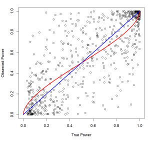
YM figure2

The most important observation is that observed power varies widely as a function of random sampling error in the observed effect sizes. In comparison, the systematic bias is relatively small. Moreover, observed power at the extremes clearly distinguishes between low powered (< 25%) and high powered (> 80%) power. Observed power is particularly informative when it is close to the maximum value of 100%. Thus, observed power of 99% or more strongly suggests that a study had high power. The main problem for posteriori power analysis is that observed effect sizes are imprecise estimates of the true effect size, especially in small samples. The next section examines the consequences of random sampling error in more detail.

Standard Deviation of Observed Power

Awareness has been increasing that point estimates of statistical parameters can be misleading. For example, an effect size of d = .8 suggests a strong effect, but if this effect size was observed in a small sample, the effect size is strongly influenced by sampling error. One solution to this problem is to compute a confidence interval around the observed effect size. The 95% confidence interval is defined by sampling error times 1.96; approximately 2. With sampling error of .4, the confidence interval could range all the way from 0 to 1.6. As a result, it would be misleading to claim that an effect size of d = .8 in a small sample suggests that the true effect size is strong. One solution to this problem is to report confidence intervals around point estimates of effect sizes. A common confidence interval is the 95% confidence interval.   A 95% confidence interval means that there is a 95% probability that the population effect size is contained in the 95% confidence interval around the (biased) effect size in a sample.

To illustrate the use of confidence interval, I computed the confidence interval for the example of music training and IQ in children. The example assumes that the IQ of 100 children after a music intervention is 103. After subtracting the population mean of 100 and dividing by the standard deviation of 15, the effect size is d = 3/15 = .2. Sampling error is defined by 1 / sqrt (n). With a sample size of n = 100, sampling error is .10. To compute a 95% confidence interval, sampling error is multiplied with the z-scores that capture 95% of a standard normal distribution, which is 1.96.   As sampling error is .10, the values are -.196 and .196.   Given an observed effect size of d = .2, the 95% confidence interval ranges from .2 – .196 = .004 to .2 + .196 = .396.

A confidence interval can be used for significance testing by examining whether the confidence interval includes 0. If the 95% confidence interval does not include zero, it is possible to reject the hypothesis that the effect size in the population is 0, which is equivalent to rejecting the null-hypothesis. In the example, the confidence interval ends at d = .004, which implies that the null-hypothesis can be rejected. At the upper end, the confidence interval ends at d = .396. This implies that the empirical results also would reject hypotheses that the population effect size is moderate (d = .5) or strong (d = .8).

Confidence intervals around effect sizes are also useful for posteriori power analysis. Yuan and Maxwell (2005) demonstrated that confidence interval of observed power is defined by the observed power of the effect sizes that define the confidence interval of effect sizes.

YM formula5

The figure below illustrates the observed power for the lower bound of the confidence interval in the example of music lessons and IQ (d = .004).

YM figure3

The figure shows that the non-central distribution (blue) and the central distribution (red) nearly perfectly overlap. The reason is that the observed effect size (d = .004) is just slightly above the d-value of the central distribution when the effect size is zero (d = .000). When the null-hypothesis is true, power equals the type-I error rate (2.5%) because 2.5% of studies will produce a significant result by chance alone and chance is the only factor that produces significant results. When the true effect size is d = .004, power increases to 2.74 percent.

Remember that this power estimate is based on the lower limit of a 95% confidence interval around the observed power estimate of 50%.   Thus, this result means that there is a 95% probability that the true power of the study is 2.5% when observed power is 50%.

The next figure illustrates power for the upper limit of the 95% confidence interval.
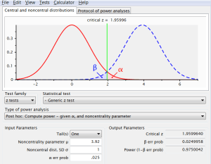
YM figure4

In this case, the non-central distribution and the central distribution overlap very little. Only 2.5% of the non-central distribution is on the left side of the criterion value, and power is 97.5%.   This finding means that there is a 95% probability that true power is not greater than 97.5% when observed power is 50%.

Taken these results together, the results show that the 95% confidence interval around an observed power estimate of 50% ranges from 2.5% to 97.5%.   As this interval covers pretty much the full range of possible values, it follows that observed power of 50% in a single study provides virtually no information about the true power of a study. True power can be anywhere between 2.5% and 97.5% percent.

The next figure illustrates confidence intervals for different levels of power.

YM figure5

The data are based on the same simulation as in the previous simulation study. The green line is based on computation of observed power for the d-values that correspond to the 95% confidence interval around the observed (simulated) d-values.

The figure shows that confidence intervals for most observed power values are very wide. The only accurate estimate of observed power can be achieved when power is high (upper right corner). But even 80% true power still has a wide confidence interval where the lower bound is below 20% observed power. Firm conclusions can only be drawn when observed power is high.

For example, when observed power is 95%, a one-sided 95% confidence interval (guarding only against underestimation) has a lower bound of 50% power. This finding would imply that observing power of 95% justifies the conclusion that the study had at least 50% power with an error rate of 5% (i.e., in 5% of the studies the true power is less than 50%).

The implication is that observed power is useless unless observed power is 95% or higher.

In conclusion, consideration of the effect of random sampling error on effect size estimates provides justification for Yuan and Maxwell’s (2005) conclusion that computation of observed power provides relatively little value.   However, the reason is not that observed power is a problematic concept. The reason is that observed effect sizes in underpowered studies provide insufficient information to estimate observed power with any useful degree of accuracy. The same holds for the reporting of observed effect sizes that are routinely reported in research reports and for point estimates of effect sizes that are interpreted as evidence for small, moderate, or large effects. None of these statements are warranted when the confidence interval around these point estimates is taken into account. A study with d = .80 and a confidence interval of d = .01 to 1.59 does not justify the conclusion that a manipulation had a strong effect because the observed effect size is largely influenced by sampling error.

In conclusion, studies with large sampling error (small sample sizes) are at best able to determine the sign of a relationship. Significant positive effects are likely to be positive and significant negative effects are likely to be negative. However, the effect sizes in these studies are too strongly influenced by sampling error to provide information about the population effect size and therewith about parameters that depend on accurate estimation of population effect sizes like power.

Meta-Analysis of Observed Power

One solution to the problem of insufficient information in a single underpowered study is to combine the results of several underpowered studies in a meta-analysis.   A meta-analysis reduces sampling error because sampling error creates random variation in effect size estimates across studies and aggregation reduces the influence of random factors. If a meta-analysis of effect sizes can produce more accurate estimates of the population effect size, it would make sense that meta-analysis can also increase the accuracy of observed power estimation.

Yuan and Maxwell (2005) discuss meta-analysis of observed power only briefly.

YM figure6

A problem in a meta-analysis of observed power is that observed power is not only subject to random sampling error, but also systematically biased. As a result, the average of observed power across a set of studies would also be systematically biased.   However, the reason for the systematic bias is the non-symmetrical distribution of observed power when power is not 50%.   To avoid this systematic bias, it is possible to compute the median. The median is unbiased because 50% of the non-central distribution is on the left side of the non-centrality parameter and 50% is on the right side of the non-centrality parameter. Thus, the median provides an unbiased estimate of the non-centrality parameter and the estimate becomes increasingly accurate as the number of studies in a meta-analysis increases.

The next figure shows the results of a simulation with the same 500 studies (25 sample sizes and 20 effect sizes) that were simulated earlier, but this time each study was simulated to be replicated 1,000 times and observed power was estimated by computing the average or the median power across the 1,000 exact replication studies.

YM figure7

Purple = average observed power;   Orange = median observed power

The simulation shows that Yuan and Maxwell’s (2005) bias formula predicts the relationship between true power and the average of observed power. It also confirms that the median is an unbiased estimator of true power and that observed power is a good estimate of true power when the median is based on a large set of studies. However, the question remains whether observed power can estimate true power when the number of studies is smaller.

The next figure shows the results for a simulation where estimated power is based on the median observed power in 50 studies. The maximum discrepancy in this simulation was 15 percentage points. This is clearly sufficient to distinguish low powered studies (<50% power) from high powered studies (>80%).

YM figure8

To obtain confidence intervals for median observed power estimates, the power estimate can be converted into the corresponding non-centrality parameter of a standard normal distribution. The 95% confidence interval is defined as the standard deviation divided by the square root of the number of studies. The standard deviation of a standard normal distribution equals 1. Hence, the 95% confidence interval for a set of studies is defined by

Lower Limit = Normal (InverseNormal (power) – 1.96 / sqrt(k))

Upper Limit = Normal (inverseNormal(power) + 1.96 / sqrt(k))

Interestingly, the number of observations in a study is irrelevant. The reason is that larger samples produce smaller confidence intervals around an effect size estimate and increase power at the same time. To hold power constant, the effect size has to decrease and power decreases exponentially as effect sizes decrease. As a result, observed power estimates do not become more precise when sample sizes increase and effect sizes decrease proportionally.

The next figure shows simulated data for 1000 studies with 20 effect sizes (0.05 to 1) and 25 sample sizes (n = 10 to 250). Each study was repeated 50 times and the median value was used to estimate true power. The green lines are the 95% confidence interval around the true power value.   In real data, the confidence interval would be drawn around observed power, but observed power does not provide a clear mathematical function. The 95% confidence interval around the true power values is still useful because it predicts how much observed power estimates can deviate from true power. 95% of observed power values are expected to be within the area that is defined by lower and upper bound of the confidence interval. The Figure shows that most values are within the area. This confirms that sampling error in a meta-analysis of observed power is a function of the number of studies. The figure also shows that sampling error is greatest when power is 50%. In the tails of the distribution range restriction produces more precise estimates more quickly.

YM figure9

With 50 studies, the maximum absolute discrepancy is 15 percentage points. This level of precision is sufficient to draw broad conclusions about the power of a set of studies. For example, any median observed power estimate below 65% is sufficient to reveal that a set of studies had less power than Cohen’s recommended level of 80% power. A value of 35% would strongly suggest that a set of studies was severely underpowered.

Conclusion

Yuan and Maxwell (2005) provided a detailed statistical examination of observed power. They concluded that observed power typically provides little to no useful information about the true power of a single study. The main reason for this conclusion was that sampling error in studies with low power is too large to estimate true power with sufficient precision. The only precise estimate of power can be obtained when sampling error is small and effect sizes are large. In this case, power is near the maximum value of 1 and observed power correctly estimates true power as being close to 1. Thus, observed power can be useful when it suggests that a study had high power.

Yuan and Maxwell’s (2005) also showed that observed power is systematically biased unless true power is 50%. The amount of bias is relatively small and even without this systematic bias, the amount of random error is so large that observed power estimates based on a single study cannot be trusted.

Unfortunately, Yuan and Maxwell’s (2005) article has been misinterpreted as evidence that observed power calculations are inherently biased and useless. However, observed power can provide useful and unbiased information in a meta-analysis of several studies. First, a meta-analysis can provide unbiased estimates of power because the median value is an unbiased estimator of power. Second, aggregation across studies reduces random sampling error, just like aggregation across studies reduces sampling error in meta-analyses of effect sizes.

Implications

The demonstration that median observed power provides useful information about true power is important because observed power has become a valuable tool in the detection of publication bias and other biases that lead to inflated estimates of effect sizes. Starting with Sterling, Rosenbaum, and Weinkam ‘s(1995) seminal article, observed power has been used by Ioannidis and Trikalinos (2007), Schimmack (2012), Francis (2012), Simonsohn (2014), and van Assen, van Aert, and Wicherts (2014) to draw inferences about a set of studies with the help of posteriori power analysis. The methods differ in the way observed data are used to estimate power, but they all rely on the assumption that observed data provide useful information about the true power of a set of studies. This blog post shows that Yuan and Maxwell’s (2005) critical examination of observed power does not undermine the validity of statistical approaches that rely on observed data to estimate power.

Future Directions

This blog post focussed on meta-analysis of exact replication studies that have the same population effect size and the same sample size (sampling error). It also assumed that the set of studies is a representative set of studies. An important challenge for future research is to examine the statistical properties of observed power when power varies across studies (heterogeneity) and when publication bias and other biases are present. A major limitation of existing methods is that these methods assume a fixed population effect size (Ioannidis and Trikalinos (2007), Francis (2012), Simonsohn (2014), and van Assen, van Aert, and Wicherts (2014). At present, the Incredibility index (Schimmack, 2012) and the R-Index (Schimmack, 2014) have been proposed as methods for sets of studies that are biased and heterogeneous. An important goal for future research is to evaluate these methods in simulation studies with heterogeneous and biased sets of data.


Power Failure in Neuroscience

Original: December 5, 2014
Revised: December 28, 2020

Power Failure in Neuroscience

An article in Nature Review” Neuroscience suggested that the median power in neuroscience studies is just 21% (Katherine S. Button, John P. A. Ioannidis, Claire Mokrysz, Brian A.Nosek, Jonathan Flint, Emma S.J. Robinson and Marcus R. Munafò, 2013).

The authors of this article examined meta-analyses of primary studies in neuroscience that were published in 2011. They analyzed 49 meta-analyses that were based on a total of 730 original studies (on average, 15 studies per meta-analysis, range 2 to 57).

For each primary study, the authors computed observed power based on the sample size and the estimated effect size in the meta-analysis.

Based on their analyses, the authors concluded that the median power in neuroscience is 21%.

There is a major problem with this estimate that the authors overlooked. The power estimate is incredibly low because a median power estimate of 21% corresponds to a p-value of p = .25. If median power were 21%, it would mean that over 50% of the original studies in the meta-analysis reported a non-significant result (p > .05). This seems rather unlikely because journals tend to publish mostly significant results.

The estimate is even less plausible because it is based on meta-analytic averages without any correction for bias. These effect sizes are likely to be inflated, which means that median power estimate is inflated. Thus, true power is even less than 21% and even more results are non-significant.

What could explain this implausible result?

  1. A meta-analysis includes published and unpublished studies. It is possible that the published studies reported significant results with observed power greater than 50% (p < .05) and the unpublished studies reported non-significant results with power less than 50%. However, this would imply that meta-analysts were able to retrieve as many unpublished studies as published studies. The authors did not report whether power of published and unpublished studies differed.
  2. A second possibility is that the power analyses produced false results. The authors relied on Ioannidis and Trikalinos’s (2007) approach to the estimation of power. This approach assumes that studies in a meta-analysis have the same true effect size and that the meta-analytic average (weighted mean) provides the best estimate of the true effect size. This estimate of the true effect size is then used to estimate power in individual studies based on the sample size of the study. As already noted by Ioannidis and Trikalinos (2007), this approach can produce biased results when effect sizes in a meta-analysis are heterogeneous.
  3. Estimating power simply on the basis of effect size and sample size can be misleading when the design is not a simple comparison of two groups. Between-subject designs are common in animal studies in neuroscience. However, many fMRI studies use within-subject designs that achieve high statistical power with a few participants because participants serve as their own controls.

Schimmack (2012) proposed an alternative procedure that does not have this limitation. Power is estimated individually for each study based on the observed effect size in this study. This approach makes it possible to estimate median power for heterogeneous sets of studies with different effect sizes. Moreover, this approach makes it possible to compute power when power is not simply a function of sample size and effect size (e.g., within-subject designs).

R-Index of Nature Neuroscience: Analysis

To examine the replicability of research published in nature and neuroscience, I retrieved the most cited articles in this journal until I had a sample of 20 studies. I needed 14 articles to meet this goal. The number of studies in these articles ranged from 1 to 7.

The success rate for focal significance tests was 97%. This implies that the vast majority of significance tests reported a significant result. The median observed power was 84%. The inflation rate is 13% (97% – 84% = 13%). The R-Index is 71%. Based on these numbers, the R-Index predicts that the majority of studies in nature neuroscience would replicate in an exact replication study.

This conclusion differs dramatically from Button et al.’s (2013) conclusion. I therefore examined some of the articles that were used for Button et al.’s analyses.

A study by Davidson et al. (2003) examined treatment effects in 12 depressed patients and compared them to 5 healthy controls. The main findings in this article were three significant interactions between time of treatment and group with z-scores of 3.84, 4.60, and 4.08. Observed power for these values with p = .05 is over 95%. If a more conservative significance level of p = .001 is used, power is still over 70%. However, the meta-analysis focused on the correlation between brain activity at baseline and changes in depression over time. This correlation is shown with a scatterplot without reporting the actual correlation or testing it for significance. The text further states that a similar correlation was observed for an alternative depression measure with r = .46 and noting correctly that this correlation is not significant, t(10) = 1.64, p = .13, d = .95, obs. power = 32%. The meta-analysis found a mean effect size of .92. A power analysis with d = .92 and N = 12 yields a power estimate of 30%. Presumably, this is the value that Button et al. used to estimate power for the Davidson et al. (2003) article. However, the meta-analysis did not include the more powerful analyses that compared patients and controls over time.

Conclusion

In the current replication crisis, there is a lot of confusion about the replicability of published findings. Button et al. (2013) aimed to provide some objective information about the replicability of neuroscience research. They concluded that replicability is very low with a median estimate of 21%. In this post, I point out some problems with their statistical approach and the focus on meta-analyses as a way to make inferences about replicability of published studies. My own analysis shows a relatively high R-Index of 71%. To make sense of this index it is instructive to compare it to the following R-Indices.

In a replication project of psychological studies, I found an R-Index of 43% and 28% of studies were successfully replicated.

In the many-labs replication project, 10 out of 12 studies were successfully replicated, a replication rate of 83% and the R-Index was 72%.

Caveat

Neuroscience studies may have high observed power and still not replicate very well in exact replications. The reason is that measuring brain activity is difficult and requires many steps to convert and reduce observed data into measures of brain activity in specific regions. Actual replication studies are needed to examine the replicability of published results.