Tag Archives: Feeling the Future

My email correspondence with Daryl J. Bem about the data for his “Feeling the Future”article

In 2015, Daryl J. Bem shared the datafiles for the 9 studies reported in the 2011 article “Feeling the Future” with me.  In a blog post, I reported an unexplained decline effect in the data.  In an email exchange with Daryl Bem, I asked for some clarifications about the data, comments on the blog post, and permission to share the data.

Today, Daryl J. Bem granted me permission to share the data.  He declined to comment on the blog post and did not provide an explanation for the decline effect.  He also did not comment on my observation that the article did not mention that “Experiment 5” combined two experiments with N = 50 and that “Experiment 6” combined three datasets with Ns = 91, 19, and 40.  It is highly unusual to combine studies and this practice contradicts Bem’s claim that sample sizes were determined a priori based on power analysis.

Footnote on p. 409. “I set 100 as the minimum number of participants/sessions for each of the experiments reported in this article because most effect sizes (d) reported in the
psi literature range between 0.2 and 0.3. If d = 0.25 and N = 100, the power
to detect an effect significant at .05 by a one-tail, one-sample t test is .80
(Cohen, 1988).”

The undisclosed concoction of datasets is another questionable research practice that undermines the scientific integrity of significance tests reported in the original article. At a minimum, Bem should issue a correction that explains how the nine datasets were created and what decision rules were used to stop data collection.

I am sharing the datafiles so that other researchers can conduct further analyses of the data.

Datafiles: EXP1   EXP2   EXP3   EXP4   EXP5   EXP6   EXP7   EXP8   EXP9

Below is the complete email correspondence with Daryl J. Bem.

=======================================================

From: Daryl J. Bem
To: Ulrich Schimmack
Sent: Wednesday, February 25, 2015 2:47 AM

Dear Dr. Schimmack,

Attached is a folder of the data from my nine “Feeling the Future” experiments.  The files are plain text files, one line for each session, with variables separated by tabs.  The first line of each file is the list of variable names, also separated by tabs. I have omitted participants’ names but supplied their sex and age.

You should consult my 2011 article for the descriptions and definitions of the dependent variables for each experiment.

Most of the files contain the following variables: Session#, Date, StartTime, Session Length, Participant’s Sex, Participant’s Age, Experimenter’s Sex,  [the main dependent variable or variables], Stimulus Seeking score (from 1 to 5).

For the priming experiments (#3 & #4), the dependent variables are LnRT Forward and LnRT Retro, where Ln is the natural log of Response Times. As described in my 2011 publication, each response time (RT) is transformed by taking the natural log before being entered into calculations.  The software subtracts the mean transformed RT for congruent trials from the mean Transformed RT for incongruent trials, so positive values of LnRT indicate that the person took longer to respond to incongruent trials than to congruent trials.  Forward refers to the standard version of affective priming and Retro refers to the time-reversed version.  In the article, I show the results for both the Ln transformation and the inverse transformation (1/RT) for two different outlier definitions.  In the attached files, I provide the results using the Ln transformation and the definition of a too-long RT outlier as 2500 ms.

Subjects who made too many errors (> 25%) in judging the valence of the target picture were discarded. Thus, 3 subjects were discarded from Experiment #3 (hence N = 97) and 1 subject was discarded from Experiment #4 (hence N  = 99).  Their data do not appear in the attached files.

Note that the habituation experiment #5 used only negative and control (neutral) stimuli.

Habituation experiment #6 used Negative, erotic, and Control (neutral) stimuli.

Retro Boredom experiment #7 used only neutral stimuli.

In Experiment #8, the first  Retro Recall, the first 100 sessions are experimental sessions.  The last 25 sessions are no-practice control sessions.  The type of session is the second variable listed.

In Experiment #9, the first 50 sessions are the experimental sessions and the last 25 are no-practice control sessions.   Be sure to exclude the control sessions when analyzing the main experimental sessions. The summary measure of psi performance is the Precog% Score (DR%) whose definition you will find on page 419 of my article.

Let me know if you encounter any problems or want additional data.

Sincerely,
Daryl J.  Bem
Professor Emeritus of Psychology

================================================

3 years later, ….

================================================

From: Ulrich Schimmack
To: Daryl J. Bem
Sent: Wednesday, January 3, 2018 4:12 PM

Dear Dr. Bem,

I am finally writing up the results of my reanalyses of your ESP studies.

I encountered one problem with the data for Study 6.

I cannot reproduce the test results reported in the article.

The article :

Both retroactive habituation hypothesis were supported. On trials with negative picture pairs, participants preferred the target significantly more frequently than the nontarget, 51.8%, t(149) _ 1.80, p _ .037, d _ 0.15, binomial z _ 1.74, p _ .041, thereby providing a successful replication of Experiment 5. On trials with erotic picture pairs, participants preferred the target significantly less frequently than the nontarget, 48.2%, t(149) _ _1.77, p _.039, d _ 0.14, binomial z _ _1.74, p _ .041.

I obtain

(negative)
t = 1.4057, df = 149, p-value = 0.1619

(erotic)
t = -1.3095, df = 149, p-value = 0.1924

Also, I wonder why the first 100 cases often produce decimals of .25 and the last 50 cases produce decimals of .33.

It would be nice if you could look into this and let me know what could explain the discrepancy.

Best,
Uli Schimmack

=========================================

From: Ulrich Schimmack
To: Daryl J. Bem
Sent: Saturday, January 6, 2018 11:43 AM

Dear Dr. Bem,

Please reply as soon as possible to my email.  Other researchers are interested in analyzing the data and if I submit my analyses some journals want me to provide data or an explanation why I cannot share the data.  I hope to hear from you by the end of this week.

Best, Dr. Schimmack

———————————————————–

From: Ulrich Schimmack
To: Daryl J. Bem
Sent: Saturday, January 6, 2018 11:43 AM

Dear Dr. Bem,

Meanwhile I posted a blog post about your 2011 article.  It has been well received by the scientific community.  I would like to encourage you to comment on it.

https://replicationindex.com/2018/01/05/why-the-journal-of-personality-and-social-psychology-should-retract-article-doi-10-1037-a0021524-feeling-the-future-experimental-evidence-for-anomalous-retroactive-influences-on-cognition-a/

Best,
Dr. Schimmack

=====================================================

From: Daryl J. Bem
To: Ulrich Schimmack
Sent: Wednesday, January 10, 2018 4:42 PM

Dear Dr. Schimmack,

Sorry for the delay.  I have been busy re-programming my new experiments so they can be run online, requiring me to relearn the programming language.

The confusion you have experienced arises because the data from Experiments 5 and 6 in my article were split differently for exposition purposes. If you read the report of those two experiments in the article, you will see that Experiment 5 contained 100 participants experiencing only negative (and control) stimuli.  Experiment contained 150 participants who experienced negative, erotic, and control stimuli.

I started Experiment 5 (my first precognitive experiment) in the Spring semester of 2002. I ran the pre-planned 100 sessions, using only negative and control stimuli.  During that period, I was alerted to the 2002 publication by Dijksterhuis & Smith in the journal Emotion, in which they claimed to demonstrate the reverse of the standard “familiarity-promotes-liking” effect, showing that people also adapt to stimuli that are initially very positive and hence become less attractive as the result of multiple exposures.

So after completing my 100 sessions, I used what remained of the Spring semester to design and run a version of my own retroactive experiment that included erotic stimuli in addition to the negative and control stimuli.  I was able to run 50 sessions before the Spring semester ended, and I resumed that extended version the experiment in the following Fall semester when student-subjects again became available until I had a total of 150 sessions of this extended version.  For purposes of analysis and exposition, I then divided the experiments as described in the article:  100 sessions with only negative stimuli and 150 sessions with negative and erotic stimuli.  No subjects or sessions have been added or omitted, just re-assembled to reflect the change in protocol.

I don’t remember how I sent you the original data, so I am attaching a comma-delimited file (which will open automatically in Excel if you simply double or right click it).  It contains all 250 sessions ordered by dates.  The fields provided are:  Session number (numbered from 1 to 250 in chronological order),  the date of the session, the sex of the participant, % of hits on negative stimuli, % of hits on erotic stimuli (which is blank for the 100 subjects in Experiment 5) and % of hits on neutral stimuli.

Let me know if you need additional information.

I hope to get to your blog post soon.

Best,
Daryl Bem

———————————————————–

From: Ulrich Schimmack
To: Daryl J. Bem
Sent: Wednesday, January 10, 2018 5:03 PM

Dear Dr. Bem,

Frequencies of male and female in dataset 5.

> table(bem5$Participant.Sex)

Female   Male
63     37

Article “One hundred Cornell undergraduates, 63 women and 37 men,
were recruited through the Psychology Department’s”

Analysis of dataset 5

One Sample t-test
data:  bem5$N.PC.C.PC[b:e]
t = 2.7234, df = 99, p-value = 0.007639
alternative hypothesis: true mean is not equal to 0
95 percent confidence interval:
1.137678 7.245655
sample estimates:
mean of  x
4.191667

Article “t(99) =  2.23, p = .014”

Conclusion:
Gender of participants matches.
t-values do not match, but both are significant.

Frequencies of male and female in dataset 6.

> table(bem6$Participant.Sex)

Female   Male
87     63

Article: Experiment 6: Retroactive Habituation II
One hundred fifty Cornell undergraduates, 87 women and 63
men,

Negative

Paired t-test
data:  bem6$NegHits.PC and bem6$ControlHits.PC
t = 1.4057, df = 149, p-value = 0.1619
alternative hypothesis: true difference in means is not equal to 0
95 percent confidence interval:
-0.8463098  5.0185321
sample estimates:
mean of the differences
2.086111

Erotic

Paired t-test
data:  bem6$EroticHits.PC and bem6$ControlHits.PC
t = -1.3095, df = 149, p-value = 0.1924
alternative hypothesis: true difference in means is not equal to 0
95 percent confidence interval:
-4.2094289  0.8538733
sample estimates:
mean of the differences
-1.677778

Article

Both retroactive habituation hypothesis were supported. On
trials with negative picture pairs, participants preferred the target
significantly more frequently than the nontarget, 51.8%, t(149) _
1.80, p _ .037, d _ 0.15, binomial z _ 1.74, p _ .041, thereby
providing a successful replication of Experiment 5. On trials with
erotic picture pairs, participants preferred the target significantly
less frequently than the nontarget, 48.2%, t(149) _ _1.77, p _
.039, d _ 0.14, binomial z _ _1.74, p _ .041.

Conclusion:
t-values do not match, article reports significant results, but data you shared show non-significant results, although gender composition matches article.

I will double check the datafiles that you sent me in 2015 against the one you are sending me now.

Let’s first understand what is going on here before we discuss other issues.

Best, Dr. Schimmack

———————————————————–

From: Ulrich Schimmack
To: Daryl J. Bem
Sent: Wednesday, January 10, 2018 5.41 PM

Dear Dr. Bem,

I just double checked the data you sent me today and they match the data you sent me in 2015.

This means neither of these datasets reproduces the results reported in your 2011 article.

This means your article reported two more significant results (Study 6, Negative and Erotic) than the data support.

This raises further concerns about the credibility of your published results, in addition to the decline effect that I found in your data (except in Study 6, which also produced non-significant results).

Do you still believe that your 2011 studies provided credible information about timer-reversed causality or do you think that you may have capitalized on chance by conducting many pilot studies?

Best, Dr. Schimmack

=======================================

From: Daryl J. Bem
To: Ulrich Schimmack
Sent: Thursday, January 11, 2018 10.53 PM

I’ll check them tomorrow to see where the problems are.

==========================================

From: Ulrich Schimmack
To: Daryl J. Bem
Sent: Friday, January 12, 2018 11.08 AM

Dear Dr. Bem,

I conducted further analyses and I figured out why I obtained discrepant results for Study 6.

I computed difference scores with the control condition, but the article reports results for a one-sample t-test of the hit rates against an expected value of 50%.

I also figured out that the first 91 participants were exposed to 16 critical trials and participants 92 to 150 were exposed to 30 critical trials. Can you please confirm this?

Best, Dr. Schimmack

—————————————————————–

From: Daryl J. Bem
To: Ulrich Schimmack
Sent: Friday, January 12, 2018 2.17 PM

Dear Dr. Schimmack,

You are correct that I calculated all hit rates against a fixed null of 50%.

You are also correct that the first 91 participants (Spring semester of 2002) were exposed to 48 trials: 16 Negative images, 16, Erotic images, and 16 Neutral Images.

We continued with that same protocol in the Fall semester of 2002 for 19 additional sessions, sessions 51-91.

At this point, it was becoming clear from post-session debriefings of participants that the erotic pictures from the Affective Picture System (IAPS) were much too mild, especially for male participants.

(Recall that this was chronologically my first experiment and also the first one to use erotic materials.  The observation that mild erotic stimuli are insufficiently arousing, at least for college students, was later confirmed in our 2016 meta-analysis, which found that Wagenmakers attempt to replicate my Experiment #1 (Which of two curtains hides an erotic picture?) using only mild erotic pictures was the only replication failure out of 11 replication attempts of that protocol in our database.)  In all my subsequent experiments with erotic materials, I used the stronger images and permitted participants to choose which kind of erotic images (same-sex vs. opposite-sex erotica) they would be seeing.

For this reason, I decided to introduce more explicit erotic pictures into this attempted replication of the habituation protocol.

In particular, Sessions 92-110 (19 sessions) also consisted of 48 trials, but they were divided into 12 Negative trials, 12 highly Erotic trials, & 24 Neutral trials.

Finally, Sessions 111-150 (40 sessions) increased the number of trials to 60:  15 Negative trials, 15 Highly Erotic trials, & 30 Neutral trials.  With the stronger erotic materials, we felt we needed to have relatively more neutral stimuli interspersed with the stronger erotic materials.

Best,
Daryl Bem

——————————————————————-

From: Ulrich Schimmack
To: Daryl J. Bem
Sent: Friday, January 12, 2018 7.01 PM

Dear Dr. Bem,

Now that my question about Study 6 has been answered, I would like to hear your thoughts about my blog post. How do you explain the decline effect in your data; that is effect sizes decrease over the course of each experiment and when two experiments are combined into a single dataset, the decline effect seems to repeat at the beginning of the new study.   Study 6, your earliest study, doesn’t show the effect, but most other studies show this pattern.  As I pointed out on my blog, I think there are two explanations (see also Schooler, 2011).  Either unpublished studies with negative results were omitted or measurement of PSI makes the effect disappear.  What is probably most interesting is to know what you did when you encountered a promising pilot study.  Did you then start collecting new data with this promising procedure or did you continue collecting data and retained the pilot data?

Best, Dr. Schimmack

———————————————————————

From: Ulrich Schimmack
To: Daryl J. Bem
Sent: Friday, January 12, 2018 7.47 PM

Dear. Dr. Bem,

Also, is it ok for me to share your data in public or would you rather post them in public?

Best, Dr. Schimmack

===================================================

From: Ulrich Schimmack
To: Daryl J. Bem
Sent: Saturday, January 13, 2018 2.42 PM

Dear Dr. Bem,

I wrote another blog post about Study 6.  If you have any comments about this blog post or the earlier blog post, please let me know.

Also, other researchers are interested in looking at the data and I still need to hear from you how to share the datafiles.

Best, Dr. Schimmack

[Attachment: Draft of Blog Post]

————————————————————————–

From: Ulrich Schimmack
To: Daryl J. Bem
Sent: Saturday, January 13, 2018 3.53 PM

Dear Dr. Bem,

I put together a table that summarizes when studies were done and how they were combined into datasets.

Please confirm that this is accurate or let me know if there are any mistakes.

Best, Dr. Schimmack

Dataset Sample Year N
5 1 2002 50
5 2 2002 50
6 1 2002 91
6 2 2002 19
6 3 2002 40
7 1 2005 200
1 1 2006 40
1 2 2006 60
3 1 2007 100
8 1 2007 100
2 1 2008 100
2 2 2008 50
4 1 2008 100
9 1 2009 50

================================================

From: Ulrich Schimmack
To: Daryl J. Bem
Sent: Monday, January 15, 2018 10.46 AM

Dear Dr. Bem,

I am sorry to bother you with my requests. It would be helpful if you could let me know if you are planning to respond to my questions and if so, when you will be able to do so?

Best regards,
Dr. Ulrich Schimmack

————————————————————————–

From: Daryl J. Bem
To: Ulrich Schimmack
Sent: Monday, January 15, 2018, 4.17 PM

Dear Dr. Schimmack,

Here is my analysis of your Table.  I will try to get to the rest of your commentary in the coming week.

Attached Word document:

Dear Dr. Schimmack,

In looking at your table, I wasn’t sure from your numbering of Datasets & Samples which studies corresponded to those reported in my Feeling the Future article.  So I have prepared my own table in the same ordering you have provided and added a column identifying the phenomenon under investigation  (It is on the next page)

Unless I have made a mistake in identifying them, I find agreement between us on most of the figures.  I have marked in red places where we seem to disagree, which occur on Datasets identified as 3 & 8.  You have listed the dates for both as 2007, whereas my datafiles have 2008 listed for all participant sessions which describe the Precognitive Avoidance experiment and its replication.  Perhaps I have misidentified the two Datasets.  The second discrepancy is that you have listed Dataset 8 as having 100 participants, whereas I ran only 50 sessions with a revised method of selecting the negative stimulus for each trial.  As noted in the article, this did not produce a significant difference in the size of the effect, so I included all 150 sessions in the write-up of that experiment.

I do find it useful to identify the Datasets & Samples with their corresponding titles in the article.  This permits readers to read the method sections along with the table.  Perhaps it will also identify the discrepancy between our Tables.  In particular, I don’t understand the separation in your table between Datasets 8 & 9.  Perhaps you have transposed Datasets 4 & 8.

If so, then Datasets 4 & 9 would each comprise 50 sessions.

More later.

Your Table:

Dataset Sample    Year       N
5              1              2002       50
5              2              2002       50
6              1              2002       91
6              2              2002       19
6              3              2002       40
7              1              2005       200
1              1              2006       40
1              2              2006       60
3              1              2007       100
8              1              2007       100
2              1              2008       100
2              2              2008       50
4              1              2008       100
9              1              2009       50

My Table:

Dataset Sample    Year       N             Experiment
5              1              2002       50           #5: Retroactive Habituation I (Neg only)
5              2              2002       50           #5: Retroactive Habituation I (Neg only)
6              1              2002       91          #6: Retroactive Habituation II (Neg & Erot)
6              2              2002       19           #6: Retroactive Habituation II (Neg & Erot)
6              3              2002       40          #6: Retroactive Habituation II (Neg & Erot)
7              1              2005       200         #7: Retroactive Induction of Boredom
1              1              2006       40           #1: Precognitive Detection of Erotic Stimuli
1              2              2006       60           #1: Precognitive Detection of Erotic Stimuli
3              1              2008       100         #2: Precognitive Avoidance of Negative Stimuli
8?           1              2008       50           #2: Precognitive Avoidance of Negative Stimuli
2              1              2007       100         #3: Retroactive Priming I
2              2              2008       100         #4: Retroactive Priming  II
4?           1              2008       100         #8: Retroactive Facilitation of Recall I
9              1              2009       50           #9: Retroactive Facilitation of Recall II

———————————————————

From: Ulrich Schimmack
To: Daryl J. Bem
Sent: Monday, January 15, 2018, 8.52 PM

Dear Dr. Bem,

Thank you for your table.  I think we are mostly in agreement (sorry, if I confused you by calling studies datasets. The numbers are supposed to correspond to the experiment numbers in your table.

The only remaining inconsistency is that the datafile for study 8 shows year 2007, while you have 2008 in your table.

Best, Dr. Schimmack

Study    Sample    Year       N             Experiment
5              1              2002       50           #5: Retroactive Habituation I (Neg only)
5              2              2002       50           #5: Retroactive Habituation I (Neg only)
6              1              2002       91           #6: Retroactive Habituation II (Neg & Erot)
6              2              2002       19           #6: Retroactive Habituation II (Neg & Erot)
6              3              2002       40           #6: Retroactive Habituation II (Neg & Erot)
7              1              2005       200         #7: Retroactive Induction of Boredom
1              1              2006       40           #1: Precognitive Detection of Erotic Stimuli
1              2              2006       60           #1: Precognitive Detection of Erotic Stimuli
2              1              2008       100         #2: Precognitive Avoidance of Negative Stimuli
2              2              2008       50           #2: Precognitive Avoidance of Negative Stimuli
3              1              2007       100         #3: Retroactive Priming I
4              1              2008       100         #4: Retroactive Priming  II
8?           1              2007/08  100         #8: Retroactive Facilitation of Recall I
9              1              2009       50           #9: Retroactive Facilitation of Recall II

—————————————————————————

From: Daryl J. Bem
To: Ulrich Schimmack
Sent: Monday, January 15, 2018, 10.35 PM

You are correct:  Experiment 8, the first Retroactive Recall experiment was conducted in 2007 and its replication (Experiment 9) was conducted in 2009.

The Avoidance of Negative Stimuli (Study/Experiment 2)  was conducted (and reported as a single experiment with 150 sessions) in 2008.  More later.

Best,
Daryl Bem

===========================================================

From: Ulrich Schimmack
To: Daryl J. Bem
Sent: Saturday, January 20, 2018, 1.06 PM

Dear Dr. Bem,

Please let me know by tomorrow how your data should be made public.

I want to post my blog about Study 6 tomorrow. If you want to comment on it before I post it, please do so today.

Best, Dr. Schimmack

——————————————————————————————

From: Daryl J. Bem
To: Ulrich Schimmack
Sent: Saturday, January 20, 2018 5:56 PM

Dear Dr. Schimmack,

I hereby grant you permission to be the conduit for making my data available to those requesting them. Most of the researchers who contributed to our 2015/16 meta-analysis of 90 retroactive “feeling-the-future” experiments have already received the data they required for replicating my experiments.

At the moment, I am planning to follow up our meta-analysis of 90 experiments by setting up pre-registered studies. That seems to me to be the most profitable response to the methodological, statistical, and reporting critiques that have emerged since I conducted my original experiments more than a decade ago.  To respond to your most recent request, I am not planning at this time to write any commentary to your posts.  I am happy to let replications settle the matter.

(One minor point: I did not spend $90,000 to conduct my experiments.  Almost all of the participants in my studies at Cornell were unpaid volunteers taking psychology courses that offered (or required) participation in laboratory experiments.  Nor did I discard failed experiments or make decisions on the basis of the results obtained.)

What I did do was spend a lot of time and effort preparing and discarding early versions of written instructions, stimulus sets and timing procedures.  These were pretested primarily on myself and my graduate assistants, who served repeatedly as pilot subjects. If instructions or procedures were judged to be too time consuming, confusing, or not arousing enough, they were changed before the formal experiments were begun on “real” participants.  Changes were not made on the basis of positive or negative results because we were only testing the procedures on ourselves.

When I did decide to change a formal experiment after I had started it, I reported it explicitly in my article. In several cases I wrote up the new trials as a modified replication of the prior experiment.  That’s why there are more experiments than phenomena in my article:  2 approach/avoidance experiments, 2 priming experiments, 3 habituation experiments, & 2 recall experiments.)

In some cases the literature suggested that some parameters would be systematically related to the dependent variables in nonlinear fashion—e.g., the number of subliminal presentations used in the familiarity-produces-increased liking effect, which has a curvilinear relationship.  In that case, I incorporated the variable as a systematic independent variable. That is also reported in the article.

It took you approximately 3 years to post your responses to my experiments after I sent you the data.  Understandable for a busy scholar.  But a bit unziemlich for you to then send me near-daily reminders the past 3 weeks to respond back to you (as Schumann commands in the first movement of his piano Sonata in g Minor) “so schnell wie möglich!”  And then a page later, “Schneller!”

Solche Unverschämtheit!   Wenn ich es sage.

Daryl J.  Bem
Professor Emeritus of Psychology

——————————————————————–

From: Ulrich Schimmack
To: Daryl J. Bem
Sent: Saturday, January 20, 2018 6:48 PM

Dear Dr. Bem,

Thank you for your final response.   It answers all of my questions.

I am sorry if you felt bothered by my emails, but I am confident that many psychologists are interested in your answers to my questions.

Best, Dr. Schimmack

============================================

From: Ulrich Schimmack
To: Daryl J. Bem
Sent: Thursday, January 25, 2018 12:05 PM

Dear Dr. Bem,

I now started working on the meta-analysis.
I see another study by you listed (Bem, 2012, N = 42).
Can you please send me the original data for this study?

Best, Dr. Schimmack

———————————————————————————

From: Daryl J. Bem
To:  Ulrich Schimmack
Sent: Thursday,  January 25, 2018 4:45 PM

Dear Dr. Schimmack,

You reference Schooler who has documented the decline effect in several areas—not just in psi research—and has advanced some hypotheses about its possible causes.  The hypothesis that strikes me as most plausible is that it is an experimenter effect whereby experimenters and their assistants begin with high expectations and enthusiasm begin to get bored after conducting a lot of sessions.  This increasing lack of enthusiasm gets transmitted to the participants during the sessions.  I also refer you to Bob Rosenthal’s extensive work with experimenter effects—which show up even in studies with maze-running rats.

Most of Galak’s sessions were online, thereby diminishing this factor.  Now that I am retired and no longer have a laboratory with access to student assistants and participants, I, too, am shifting to online administration, so it will provide a rough test of this hypothesis.

Were you planning to publish our latest exchange concerning the meta-analysis?  I would not like to leave your blog followers with only your statement that it was “contaminated” by my own studies when, in fact, we did a separate meta-analysis on the non-Bem replications, as I noted in my previous email to you.

Best,
Daryl Bem

————————————————————————-

From: Daryl J. Bem
To:  Ulrich Schimmack
Sent: Thursday,  January 25, 2018 4:45 PM

Dear Dr. Shimmack,

I was not able to figure out how to leave a comment on your blog post at the website. (I kept being asked to register a site of my own.)  So, I thought I would simply write you a note.  You are free to publish it as my response to your most recent post if you wish.

In reading your posts on my precognitive experiments, I kept puzzling over why you weren’t mentioning the published Meta-analysis of 90 “Feeling the Future” studies that I published in 2015 with Tessoldi, Rabeyron, & Duggan. After all, the first question we typically ask when controversial results are presented is  “Can Independent researchers replicate the effect(s)?”  I finally spotted a fleeting reference to our meta-analysis in one of your posts, in which you simply dismissed it as irrelevant because it included my own experiments, thereby “contaminating” it.

But in the very first Table of our analysis, we presented the results for both the full sample of 90 studies and, separately, for the 69 replications conducted by independent researchers (from 33 laboratories in 14 countries on 10,000 participants).

These 69 (non-Bem-contaminated) independent replications yielded a z score of 4.16, p =1.2 x E-5.  The Bayes Factor was 3.85—generally considered large enough to provide “Substantial Evidence” for the experimental hypothesis.

Of these 69 studies, 31 were exact replications in that the investigators used my computer programs for conducting the experiments, thereby controlling the stimuli, the number of trials, all event timings, and automatic data recording. The data were also encrypted to ensure that no post-experiment manipulations were made on them by the experimenters or their assistants. (My own data were similarly encrypted to prevent my own assistants from altering them.) The remaining 38 “modified” independent replications variously used investigator-designed computer programs, different stimuli, or even automated sessions conducted online.

Both exact and modified replications were statistically significant and did not differ from one another.  Both peer reviewed and non-peer reviewed replications were statistically significant and did not differ from one another. Replications conducted prior to the publication of my own experiments and those conducted after their publication were each statistically significant and did not differ from one another.

We also used the recently introduced p-curve analysis to rule out several kinds of selection bias (file drawer problems), p-hacking, and to estimate “true” effect sizes.
There was no evidence of p-hacking in the database, and the effect size for the non-bem replications was 0.24, somewhat higher than the average effect size of my 11 original experiments (0.22.)  (This is also higher than the mean effect size of 0.21 achieved by Presentiment experiments in which indices of participants’ physiological arousal “precognitively” anticipate the random presentation of an arousing stimulus.)

For various reasons, you may not find our meta-analysis any more persuasive than my original publication, but your website followers might.

Best,
Daryl J.  Bem

————————————————————–

From:  Ulrich Schimmack
To: Daryl J. Bem
Sent: Thursday,  January 25, 2018 5:23 PM

Dear Dr. Bem,

I am going to share your comments on the blog.

I find the enthusiasm explanation less plausible than you.  More important, it doesn’t explain the lack of a decline effect in studies with significant results.

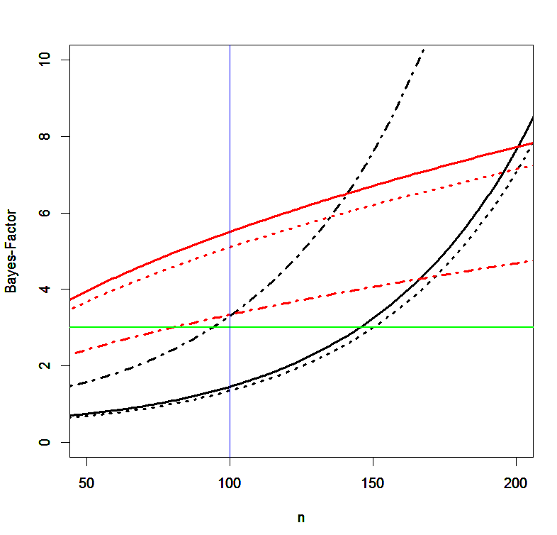
I just finished the analysis of the 6 studies with N > 100 by Maier that are also included in the meta-analysis (see Figure below).

Given the lack of a plausible explanation for your data, I think JPSP should retract your article or at least issue an expression of concern because the published results are based on abnormally strong effect sizes in the beginning of each study. Moreover, Study 5 is actually two studies of N = 50 and the pattern is repeated at the beginning of the two datasets.

I also noticed that the meta-analysis included one more study by you with an underpowered study of N = 42 that surprisingly produced yet another significant result.  As I pointed out in my article that you reviewed that you reviewed points out, this success makes it even more likely that some non-significant (pilot) studies were omitted.  Your success record is simply too good to be true (Francis, 2012).  Have you conducted any other studies since 2012?  A non-significant result is overdue.

Regarding the meta-analysis itself, most of these studies are severely underpowered and there is still evidence for publication bias after excluding your studies.

Maier.ESP.pngWhen I used puniform to control for publication bias and limited the dataset to studies with N > 90 and excluded your studies (as we agree, N < 90 is low power) the p-value was not significant, and even if it were less than .05, it would not be convincing evidence for an effect.  In addition, I computed t-values using the effect size that you assumed in 2011, d = .2, and found significant evidence against the null-hypothesis that the ESP effect size could be as large as d = .2.  This means, even studies with N = 100 are underpowered.   Any serious test of the hypothesis requires much larger sample sizes.

However, the meta-analysis and the existence of ESP are not my concern.  My concern is the way (social) psychologists have conducted research in the past and are responding to the replication crisis.  We need to understand how researchers were able to produce seemingly convincing evidence like your 9 studies in JPSP that are difficult to replicate.  How can original articles have success rates of 90% or more and replications produce only a success rate of 30% or less?  You are well aware that your 2011 article was published with reservations and concerns about the way social psychologists conducted research.   You can make a real contribution to the history of psychology by contributing to the understanding of the research process that led to your results.  This is independent of any future tests of PSI with more rigorous studies.

Best, Dr. Schimmack

=================================================

=================================================

Why Psychologists Should Not Change The Way They Analyze Their Data: The Devil is in the Default Prior

The scientific method is well-equipped to demonstrate regularities in nature as well as human behaviors. It works by repeating a scientific procedure (experiment or natural observation) many times. In the absence of a regular pattern, the empirical data will follow a random pattern. When a systematic pattern exists, the data will deviate from the pattern predicted by randomness. The deviation of an observed empirical result from a predicted random pattern is often quantified as a probability (p-value). The p-value itself is based on the ratio of the observed deviation from zero (effect size) and the amount of random error. As the signal-to-noise ratio increases, it becomes increasingly unlikely that the observed effect is simply a random event. As a result, it becomes more likely that an effect is present. The amount of noise in a set of observations can be reduced by repeating the scientific procedure many times. As the number of observations increases, noise decreases. For strong effects (large deviations from randomness), a relative small number of observations can be sufficient to produce extremely low p-values. However, for small effects it may require rather large samples to obtain a high signal-to-noise ratio that produces a very small p-value. This makes it difficult to test the null-hypothesis that there is no effect. The reason is that it is always possible to find an effect size that is so small that the noise in a study is too large to determine whether a small effect is present or whether there is really no effect at all; that is, the effect size is exactly zero (1 / infinity).

The problem that it is impossible to demonstrate scientifically that an effect is absent may explain why the scientific method has been unable to resolve conflicting views around controversial topics such as the existence of parapsychological phenomena or homeopathic medicine that lack a scientific explanation, but are believed by many to be real phenomena. The scientific method could show that these phenomena are real, if they were real, but the lack of evidence for these effects cannot rule out the possibility that a small effect may exist. In this post, I explore two statistical solutions to the problem of demonstrating that an effect is absent.

Neyman-Pearson Significance Testing (NPST)

The first solution is to follow Neyman-Pearsons’s orthodox significance test. NPST differs from the widely practiced null-hypothesis significance test (NHST) in that non-significant results are interpreted as evidence for the null-hypothesis. Thus, using the standard criterion of p = .05 as the criterion for significance, a p-value below .05 is used to reject the null-hypothesis and to infer that an effect is present. Importantly, if the p-value is greater than .05 the results are used to accept the null-hypothesis; that is, the hypothesis that there is no effect is true. As all statistical inferences, it is possible that the evidence is misleading and leads to the wrong conclusion. NPST distinguishes between two types or errors that are called type-I and type-II error. Type-I errors are errors when a p-value is below the criterion value (p < .05), but the null-hypothesis is actually true; that is there is no effect and the observed effect size was caused by a rare random event. Type-II errors are made when the null-hypothesis is accepted, but the null-hypothesis is false; there actually is an effect. The probability of making a type-II error depends on the size of the effect and the amount of noise in the data. Strong effects are unlikely to produce a type-II error even with noise data. Studies with very little noise are also unlikely to produce type-II errors because even small effects can still produce a high signal-to-noise ratio and significant results (p-values below the criterion value).   Type-II error rates can be very high in studies with small effects and a large amount of noise. NPST makes it possible to quantify the probability of a type-II error for a given effect size. By investing a large amount of resources, it is possible to reduce noise to a level that is sufficient to have a very low type-II error probability for very small effect sizes. The only requirement for using NPST to provide evidence for the null-hypothesis is to determine a margin of error that is considered acceptable. For example, it may be acceptable to infer that a weight-loss-medication has no effect on weight if weight loss is less than 1 pound over a one month period. It is impossible to demonstrate that the medication has absolutely no effect, but it is possible to demonstrate with high probability that the effect is unlikely to be more than 1 pound.

Bayes-Factors

The main difference between Bayes-Factors and NPST is that NPST yields type-II error rates for an a priori effect size. In contrast, Bayes-Factors do not postulate a single effect size, but use an a priori distribution of effect sizes. Bayes-Factors are based on the probability that the observed effect sizes is based on a true effect size of zero relative to the probability that the observed effect size was based on a true effect size within a range of a priori effect sizes. Bayes-Factors are the ratio of the probabilities for the two hypotheses. It is arbitrary, which hypothesis is in the numerator and which hypothesis is in the denominator. When the null-hypothesis is placed in the numerator and the alternative hypothesis is placed in the denominator, Bayes-Factors (BF01) decrease towards zero the more the data suggest that an effect is present. In this way, Bayes-Factors behave very much like p-values. As the signal-to-noise ratio increases, p-values and BF01 decrease.

There are two practical problems in the use of Bayes-Factors. One problem is that Bayes-Factors depend on the specification of the a priori distribution of effect sizes. It is therefore important that results can never be interpreted as evidence for the null-hypothesis or against the null-hypothesis per se. A Bayes-Factor that favors the null-hypothesis in the comparison to one a priori distribution can favor the alternative hypothesis for another a priori distribution of effect sizes. This makes Bayes-Factors impractical for the purpose of demonstrating that an effect does not exist (e.g., a drug does not have positive treatment effects). The second problem is that Bayes-Factors only provide quantitative information about the two hypotheses. Without a clear criterion value, Bayes-Factors cannot be used to claim that an effect is present or absent.

Selecting a Criterion Value for Bayes-Factors

A number of criterion values seem plausible. NPST always leads to a decision depending on the criterion for p-values. An equivalent criterion value for Bayes-Factors would be a value of 1. Values greater than 1 favor the null-hypothesis over the alternative, whereas values less than 1 favor the alternative hypothesis. This criterion avoids inconclusive results. The disadvantage with this criterion is that Bayes-Factors close to 1 are very variable and prone to have high type-I and type-II error rates. To avoid this problem, it is possible to use more stringent criterion values. This reduces the type-I and type-II error rates, but it also increases the rate of inconclusive results in noisy studies. Bayes-Factors of 3 (a 3 to 1 ratio in favor of the null over an alternative hypothesis) are often used to suggest that the data favor one hypothesis over another, and Bayes-Factors of 10 or more are often considered strong support. One problem with these criterion values is that there have been no systematic studies of the type-I and type-II error rates for these criterion values. Moreover, there have been no systematic sensitivity studies; that is, the ability of studies to reach a criterion value for different signal-to-noise ratios.

Wagenmakers et al. (2011) argued that p-values can be misleading and that Bayes-Factors provide more meaningful results. To make their point, they investigated Bem’s (2011) controversial studies that seemed to demonstrate the ability to anticipate random events in the future (time –reversed causality). Using a significance criterion of p < .05 (one-tailed), 9 out of 10 studies showed evidence of an effect. For example, in Study 1, participants were able to predict the location of erotic pictures 54% of the time, even before a computer randomly generated the location of the picture. Using a more liberal type-I error rate of p < .10 (one-tailed), all 10 studies produced evidence for extrasensory perception.

Wagenmakers et al. (2011) re-examined the data with Bayes-Factors. They used a Bayes-Factor of 3 as the criterion value. Using this value, six tests were inconclusive, three provided substantial support for the null-hypothesis (the observed effect was just due to noise in the data) and only one test produced substantial support for ESP.   The most important point here is that the authors interpreted their results using a Bayes-Factor of 3 as criterion. If they had used a Bayes-Factor of 10 as criterion, they would have concluded that all studies were inconclusive. If they had used a Bayes-Factor of 1 as criterion, they would have concluded that 6 studies favored the null-hypothesis and 4 studies favored the presence of an effect.

Matzke, Nieuwenhuis, van Rijn, Slagter, van der Molen, and Wagenmakers used Bayes-Factors in a design with optional stopping. They agreed to stop data-collection when the Bayes-Factor reached a criterion value of 10 in favor of either hypothesis. The implementation of a decision to stop data collection suggests that a Bayes-Factor of 10 was considered decisive. One reason for this stopping rule would be that it is extremely unlikely that a Bayes-Factor might swing to favoring the alternative hypothesis if more data were collected. By the same logic, a Bayes-Factor of 10 that favors the presence of an effect in an ESP effect would suggest that further data collection would be unnecessary because the evidence already shows rather strong evidence that an effect is present.

Tan, Dienes, Jansari, and Goh, (2014) report a Bayes-Factor of 11.67 and interpret as being “greater than 3 and strong evidence for the alternative over the null” (p. 19). Armstrong and Dienes (2013) report a Bayes-Factor of 0.87 and state that no conclusion follows from this finding because the Bayes-Factor is between 3 and 1/3. This statement implies that Bayes-Factors that meet the criterion value are conclusive.

In sum, a criterion-value of 3 has often been used to interpret empirical data and a criterion of 10 has been used as strong evidence in favor of an effect or in favor of the null-hypothesis.

Meta-Analysis of Multiple Studies

As sample sizes increase, noise decreases and the signal-to-noise ratio increases. Rather than increasing the sample size of a single study, it is also possible to conduct multiple smaller studies and to combine the evidence of studies in a meta-analysis. The effect is the same. A meta-analysis based on several original studies reduces random noise in the data and can produce higher signal-to-noise ratios when an effect is present. On the flip side, a low signal-to-noise ratio in a meta-analysis implies that the signal is very weak and that the true effect size is close to zero. As the evidence in a meta-analysis is based on the aggregation of several smaller studies, the results should be consistent. That is, the effect size in the smaller studies and the meta-analysis is the same. The only difference is that aggregation of studies reduces noise, which increases the signal-to-noise ratio.   A meta-analysis therefore can highlight the problem of interpreting a low signal-to-noise ratio (BF10 < 1, p > .05) in small studies as evidence for the null-hypothesis. In NPST this result would be flagged as not trustworthy because the type-II error probability is high. For example, a non-significant result with a type-II error of 80% (20% power) is not particularly interesting and nobody would want to accept the null-hypothesis with such a high error probability. Holding the effect size constant, the type-II error probability decreases as the number of studies in a meta-analysis increases and it becomes increasingly more probable that the true effect size is below the value that was considered necessary to demonstrate an effect. Similarly, Bayes-Factors can be misleading in small samples and they become more conclusive as more information becomes available.

A simple demonstration of the influence of sample size on Bayes-Factors comes from Rouder and Morey (2011). The authors point out that it is not possible to combine Bayes-Factors by multiplying Bayes-Factors of individual studies. To address this problem, they created a new method to combine Bayes-Factors. This Bayesian meta-analysis is implemented in the Bayes-Factor r-package. Rouder and Morey (2011) applied their method to a subset of Bem’s data. However, they did not use it to examine the combined Bayes-Factor for the 10 studies that Wagenmakers et al. (2011) examined individually. I submitted the t-values and sample sizes of all 10 studies to a Bayesian meta-analysis and obtained a strong Bayes-Factor in favor of an effect, BF10 = 16e7, that is, 16 million to 1 in favor of ESP. Thus, a meta-analysis of all 10 studies strongly suggests that Bem’s data are not random.

Another way to meta-analyze Bem’s 10 studies is to compute a Bayes-Factor based on the finding that 9 out of 10 studies produced a significant result. The p-value for this outcome under the null-hypothesis is extremely small; 1.86e-11, that is p < .00000000002. It is also possible to compute a Bayes-Factor for the binomial probability of 9 out of 10 successes with a probability of 5% to have a success under the null-hypothesis. The alternative hypothesis can be specified in several ways, but one common option is to use a uniform distribution from 0 to 1 (beta(1,1). This distribution allows for the power of a study to range anywhere from 0 to 1 and makes no a priori assumptions about the true power of Bem’s studies. The Bayes-Factor strongly favors the presence of an effect, BF10 = 20e9. In sum, a meta-analysis of Bem’s 10 studies strongly supports the presence of an effect and rejects the null-hypothesis.

The meta-analytic results raise concerns about the validity of Wagenmakers et al.’s (2011) claim that Bem presented weak evidence and that p-values misleading information. Instead, Wagenmakers et al.’s Bayes-Factors are misleading and fail to detect an effect that is clearly present in the data.

The Devil is in the Priors: What is the Alternative Hypothesis in the Default Bayesian t-test?

Wagenmakers et al. (2011) computed Bayes-Factors using the default Bayesian t-test. The default Bayesian t-test uses a Cauchy distribution centered over zero as the alternative hypothesis. The Cauchy distribution has a scaling factor. Wagenmakers et al. (2011) used a default scaling factor of 1. Since then, the default scaling parameter has changed to .707.Figure 1 illustrates Cauchi distributions with scaling factors .2, .5, .707, and 1.

WagF1

The black line shows the Cauchy distribution with a scaling factor of d = .2. A scaling factor of d = .2 implies that 50% of the density of the distribution is in the interval between d = -.2 and d = .2. As the Cauchy-distribution is centered over 0, this specification also implies that the null-hypothesis is considered much more likely than many other effect sizes, but it gives equal weight to effect sizes below and above an absolute value of d = .2.   As the scaling factor increases, the distribution gets wider. With a scaling factor of 1, 50% of the density distribution is within the range from -1 to 1 and 50% covers effect sizes greater than 1.   The choice of the scaling parameter has predictable consequences on the Bayes-Factor. As long as the true effect size is more extreme than the scaling parameter, Bayes-Factors will favor the alternative hypothesis and Bayes-Factors will increase towards infinity as sampling error decreases. However, for true effect sizes that are below the scaling parameter, Bayes-Factors may initially favor the null-hypothesis because the alternative hypothesis includes effect sizes that are more extreme than the alternative hypothesis. As sample sizes increase, the Bayes-Factor will change from favoring the null-hypothesis to favoring the alternative hypothesis.   This can explain why Wagenmakers et al. (2011) found no support for ESP when Bem’s studies were examined individually, but a meta-analysis of all studies shows strong evidence in favor of an effect.

The effect of the scaling parameter on Bayes-Factors is illustrated in the following Figure.

WagF2

The straight lines show Bayes-Factors (y-axis) as a function of sample size for a scaling parameter of 1. The black line shows Bayes-Factors favoring an effect of d = .2 when the effect size is actually d = .2 (BF10) and the red line shows Bayes-Factor favoring the null-hypothesis when the effect size is actually 0. The green line implies a criterion value of 3 to suggest “substantial” support for either hypothesis (Wagenmakers et al., 2011). The figure shows that Bem’s sample sizes of 50 to 150 participants could never produce substantial evidence for an effect when the observed effect size is d = .2. In contrast, an effect size of 0 would produce provide substantial support for the null-hypothesis. Of course, actual effect sizes in samples will deviated from these hypothetical values, but sampling error will average out. Thus, for studies that occasionally show support for an effect there will also be studies that underestimate support for an effect. The dotted lines illustrate how the choice of the scaling factor influences Bayes-Factors. With a scaling factor of d = .2, Bayes-Factors would never favor the null-hypothesis. They would also not support the alternative hypothesis in studies with less than 150 participants and even in these studies the Bayes-Factor is likely to be just above 3.

Figure 2 explains why Wagenmakers et al.’s (2011) did mainly find inconclusive results. On the one hand, the effect size was typically around d = .2. As a result, the Bayes-Factor did not provide clear support for the null-hypothesis. On the other hand, an effect size of d = .2 in studies with 80% power is insufficient to produce Bayes-Factors favoring the presence of an effect, when the alternative hypothesis is specified as a Cauchy distribution centered over 0. This is especially true when the scaling parameter is larger, but even for a seemingly small scaling parameter Bayes-Factors would not provide strong support for a small effect. The reason is that the alternative hypothesis is centered over 0. As a result, it is difficult to distinguish the null-hypothesis from the alternative hypothesis.

A True Alternative Hypothesis: Centering the Prior Distribution over a Non-Null Effect Size

A Cauchy-distribution is just one possible way to formulate an alternative hypothesis. It is also possible to formulate alternative hypothesis as (a) a uniform distribution of effect sizes in a fixed range (e.g., the effect size is probably small to moderate, d = .2 to .5) or as a normal distribution centered over an effect size (e.g., the effect is most likely to be small, but there is some uncertainty about how small, d = 2 +/- SD = .1) (Dienes, 2014).

Dienes provided an online app to compute Bayes-Factors for these prior distributions. I used the posted r-code by John Christie to create the following figure. It shows Bayes-Factors for three a priori uniform distributions. Solid lines show Bayes-Factors for effect sizes in the range from 0 to 1. Dotted lines show effect sizes in the range from 0 to .5. The dot-line pattern shows Bayes-Factors for effect sizes in the range from .1 to .3. The most noteworthy observation is that prior distributions that are not centered over zero can actually provide evidence for a small effect with Bem’s (2011) sample sizes. The second observation is that these priors can also favor the null-hypothesis when the true effect size is zero (red lines). Bayes-Factors become more conclusive for more precisely formulate alternative hypotheses. The strongest evidence is obtained by contrasting the null-hypothesis with a narrow interval of possible effect sizes in the .1 to .3 range. The reason is that in this comparison weak effects below .1 clearly favor the null-hypothesis. For an expected effect size of d = .2, a range of values from 0 to .5 seems reasonable and can produce Bayes-Factors that exceed a value of 3 in studies with 100 to 200 participants. Thus, this is a reasonable prior for Bem’s studies.

WagF3

It is also possible to formulate alternative hypotheses with normal distributions around an a priori effect size. Dienes recommends setting the mean to 0 and to set the standard deviation of the expected effect size. The problem with this approach is again that the alternative hypothesis is centered over 0 (in a two-tailed test).   Moreover, the true effect size is not known. Like the scaling factor in the Cauchy distribution, using a higher value leads to a wider spread of alternative effect sizes and makes it harder to show evidence for small effects and easier to find evidence in favor of H0.   However, the r-code also allows specifying non-null means for the alternative hypothesis.   The next figure shows Bayes-Factors for three normally distributed alternative hypotheses. The solid lines show Bayes-Factors with mean = 0 and SD = .2. The dotted line shows Bayes-Factors for d = .2 (a small effect and the effect predicted by Bem) and a relatively wide standard deviation of .5. This means 95% of effect sizes are in the range from -.8 to 1.2. The broken (dot/dash) line shows Bayes-Factors with a mean of d = .2 and a narrower SD of d = .2. The 95% CI still covers a rather wide range of effect sizes from -.2 to .6, but due to the normal distribution effect sizes close to the expected effect size of d = .2 are weighted more heavily.

WagF4

The first observation is that centering the normal distribution over 0 leads to the same problem as the Cauchy-distribution. When the effect size is really 0, Bayes-Factors provide clear support for the null-hypothesis. However, when the effect size is small, d = .2, Bayes-Factors fail to provide support for the presence for samples with fewer than 150 participants (this is a ones-sample design, the equivalent sample size for between-subject designs is N = 600). The dotted line shows that simply moving the mean from d = 0 to d = .2 has relatively little effect on Bayes-Factors. Due to the wide range of effect sizes, a small effect is not sufficient to produce Bayes-Factors greater than 3 in small samples. The broken line shows more promising results. With d = .2 and SD = .2, Bayes-Factors in small samples with less than 100 participants are inconclusive. For sample sizes of more than 100 participants, both lines are above the criterion value of 3. This means, a Bayes-Factor of 3 or more can support the null-hypothesis when it is true and it can show that a small effect is present when an effect is present.

Another way to specify the alternative hypothesis is to use a one-tailed alternative hypothesis (a half-normal).   The mode (the center of the normal-distribution) of the distribution is 0. The solid line shows a standard deviation of .8. The dotted line shows results with standard deviation = .5 and the broken line shows results for a standard deviation of d = .2. The solid line favors the null-hypothesis and it requires sample sizes of more than 130 participants before an effect size of d = .2 produces a Bayes-Factor of 3 or more. In contrast, the broken line discriminates against the null-hypothesis and practically never supports the null-hypothesis when it is true. The dotted line with a standard deviation of .5 works best. It always shows support for the null-hypothesis when it is true and it can produce Bayes-Factors greater than 3 with a bit more than 100 participants.

WagF5

In conclusion, the simulations show that Bayes-Factors depend on the specification of the prior distribution and sample size. This has two implications. Unreasonable priors will lower the sensitivity/power of Bayes-Factors to support either the null-hypothesis or the alternative hypothesis when these hypotheses are true. Unreasonable priors will also bias the results in favor of one of the two hypotheses. As a result, researchers need to justify the choice of their priors and they need to be careful when they interpret results. It is particularly difficult to interpret Bayes-Factors when the alternative hypothesis is diffuse and the null-hypothesis is supported. In this case, the evidence merely shows that the null-hypothesis fits the data better than the alternative, but the alternative is a composite of many effect sizes and some of these effect sizes may fit the data better than the null-hypothesis.

Comparison of Different Prior Distributions with Bem’s (2011) ESP Experiments

To examine the influence of prior distributions on Bayes-Factors, I computed Bayes-Factors using several prior distributions. I used a d~Cauchy(1) distribution because this distribution was used by Wagenmakers et al. (2011). I used three uniform prior distributions with ranges of effect sizes from 0 to 1, 0 to .5, and .1 to .3. Based on Dienes recommendation, I also used a normal distribution centered on zero with the expected effect size as the standard deviation. I used both two-tailed and one-tailed (half-normal) distributions. Based on a twitter-recommendation by Alexander Etz, I also centered the normal distribution on the effect size, d = .2, with a standard deviation of d = .2.

Wag1 Table

The d~Cauchy(1) prior used by Wagenmakers et al. (2011) gives the weakest support for an effect. The table also includes the product of Bayes-Factors. The results confirm that the product is not a meaningful statistic that can be used to conduct a meta-analysis with Bayes-Factors. The last column shows Bayes-Factors based on a traditional fixed-effect meta-analysis of effect sizes in all 10 studies. Even the d~Cauchy(1) prior now shows strong support for the presence of an effect even though it often favored the null-hypotheses for individual studies. This finding shows that inferences about small effects in small samples cannot be trusted as evidence that the null-hypothesis is correct.

Table 1 also shows that all other prior distributions tend to favor the presence of an effect even in individual studies. Thus, these priors show consistent results for individual studies and for a meta-analysis of all studies. The strength of evidence for an effect is predictable from the precision of the alternative hypothesis. The uniform distribution with a wide range of effect sizes from 0 to 1, gives the weakest support, but it still supports the presence of an effect. This further emphasizes how unrealistic the Cauchy-distribution with a scaling factor of 1 is for most studies in psychology. For most studies in psychology effect sizes greater than 1 are rare. Moreover, effect sizes greater than one do not need fancy statistics. A simple visual inspection of a scatter plot is sufficient to reject the null-hypothesis. The strongest support for an effect is obtained for the uniform distribution with a range of effect sizes from .1 to .3. The advantage of this range is that the lower bound is not 0. Thus, effect sizes below the lower bound provide evidence for H0 and effect sizes above the lower bound provide evidence for an effect. The lower bound can be set by a meaningful consideration of what effect sizes might be theoretically or practically so small that they would be rather uninteresting even if they are real. Personally, I find uniform distributions appealing because they best express uncertainty about an effect size. Most theories in psychology do not make predictions about effect sizes. Thus, it seems impossible to say that an effect is expected to be small (d = .2) or moderate (d = .5). It seems easier to say that an effect is expected to be small (d = .1 to .3) or moderate (.3 to .6) or large (.6 to 1). Cohen used fixed values only because power analysis requires a single value. As Bayesian statistics allows the specification of ranges, it makes sense to specify a range of values with the need to make predictions which values in this range are more likely. However, results for the normal distribution provide similar results. Again, the strength of evidence of an effect increases with the precision of the predicted effect. The weakest support for an effect is obtained with a normal distribution centered over 0 and a two-tailed test. This specification is similar to a Cauchy distribution but it uses the normal distribution. However, by setting the standard deviation to the expected effect sizes, Bayes-Factors show evidence for an effect. The evidence for an effect becomes stronger by centering the distribution over the expected effect size or by using a half-normal (one-tailed) test that makes predictions about the direction of the effect.

To summarize, the main point is that Bayes-Factors depend on the choice of the alternative distribution. Bayesian statisticians are of course well aware of this fact. However, in practical applications of Bayesian statistics, the importance of the prior distribution is often ignored, especially when Bayes-Factors favor the null-hypothesis. Although this finding only means that the data support the null-hypothesis more than the alternative hypothesis, the alternative hypothesis is often described in vague terms as a hypothesis that predicted an effect. However, the alternative hypothesis does not just predict that there is an effect. It makes predictions about the strength of effects and it is always possible to specify an alternative that predicts an effect that is still consistent with the data by choosing a small effect size. Thus, Bayesian statistics can only produce meaningful results if researchers specify a meaningful alternative hypothesis. It is therefore surprising how little attention Bayesian statisticians have devoted to the issue of specifying the prior distribution. The most useful advice comes from Dienes recommendation to specify the prior distribution as a normal distribution centered over 0 and to set the standard deviation to the expected effect size. If researchers are uncertain about the effect size, they could try different values for small (d = .2), moderate (d = .5), or large (d = .8) effect sizes. Researchers should be aware that the current default setting of .707 in Rouder’s online app implies an expectation of a strong effect and that this setting will make it harder to show evidence for small effects and inflates the risk of obtaining false support for the null-hypothesis.

Why Psychologists Should not Change the Way They Analyze Their Data

Wagenmakers et al. (2011) did not simply use Bayes-Factors to re-examine Bem’s claims about ESP. Like several other authors, they considered Bem’s (2011) article an example of major flaws in psychological science. Thus, they titled their article with the rather strong admonition that “Psychologists Must Change The Way They Analyze Their Data.”   They blame the use of p-values and significance tests as the root cause of all problems in psychological science. “We conclude that Bem’s p values do not indicate evidence in favor of precognition; instead, they indicate that experimental psychologists need to change the way they conduct their experiments and analyze their data” (p. 426). The crusade against p-values starts with the claim that it is easy to obtain data that reject the null-hypothesis even when the null-hypothesis is true. “These experiments highlight the relative ease with which an inventive researcher can produce significant results even when the null hypothesis is true” (p. 427). However, this statement is incorrect. The probability of getting significant results is clearly specified by the type-I error rate. When the null-hypothesis is true, a significant result will emerge only 5% of the time; that is in 1 out of 20 studies. The probability of making a type-I error repeatedly decrease exponentially. For two studies, the probability to obtain two type-I errors is only p = .0025 or 1 out of 400 (20 * 20 studies).   If some non-significant results are obtained, the binomial probability gives the probability that the frequency of significant results that could have been obtained if the null-hypothesis were true. Bem obtained 9 out of 10 significant results. With a probability of p = .05, the binomial probability is 18e-10. Thus, there is strong evidence that Bem’s results are not type-I errors. He did not just go in his lab and run 10 studies and obtained 9 significant results by chance alone. P-values correctly quantify how unlikely this event is in a single study and how this probability decrease as the number of studies increases. The table also shows that all Bayes-Factors confirm this conclusion when the results of all studies are combined in a meta-analysis.   It is hard to see how p-values can be misleading when they lead to the same conclusion as Bayes-Factors. The combined evidence presented by Bem cannot be explained by random sampling error. The data are inconsistent with the null-hypothesis. The only misleading statistic is provided by a Bayes-Factor with an unreasonable prior distribution of effect sizes in small samples. All other statistics agree that the data show an effect.

Wagenmakers et al. (2011) next argument is that p-values only consider the conditional probability when the null-hypothesis is true, but that it is also important to consider the conditional probability if the alternative hypothesis is true. They fail to mention, however, that this alternative hypothesis is equivalent to the concept of statistical power. A p-values of less than .05 means that a significant result would be obtained only 5% of the time when the null-hypothesis is true. The probability of a significant result when an effect is present depends on the size of the effect and sampling error and can be computed using standard tools for power analysis. Importantly, Bem (2011) actually carried out an a priori power analysis and planned his studies to have 80% power. In a one-sample t-test, standard error is defined as 1/sqrt(N). Thus, with 100 participants, the standard error is .1. With an effect size of d = .2, the signal-to-noise ratio is .2/.1 = 2. Using a one-tailed significance test, the criterion value for significance is 1.66. The implied power is 63%. Bem used an effect size of d = .25 to suggest that he has 80% power. Even with a conservative estimate of 50% power, the likelihood ratio of obtaining a significant is .50/.05 = 10. This likelihood ratio can be interpreted like Bayes-Factors. Thus, in a study with 50% power, it is 10 times more likely to obtain a significant result when an effect is present than when the null-hypothesis is true. Thus, even in studies with modest power, favors the alternative hypothesis much more than the null-hypothesis. To argue that p-values provide weak evidence for an effect implies that a study had very low power to show an effect. For example, if a study has only 10% power, the likelihood ratio is only 2 in favor of an effect being present. Importantly, low power cannot explain Bem’s results because low power would imply that most studies produced non-significant results. However, he obtained 9 significant results in 10 studies. This success rate is itself an estimate of power and would suggest that Bem had 90% power in his studies. With 90% power, the likelihood ratio is .90/.05 = 18. The Bayesian argument against p-values is only valid for the interpretation of p-values in a single study in the absence of any information about power. Not surprisingly, Bayesians often focus on Fisher’s use of p-values. However, Neyman-Pearson emphasized the need to also consider type-II error rates and Cohen has emphasized the need to conduct power analysis to ensure that small effects can be detected. In recent years, there has been an encouraging trend to increase power of studies. One important consequence of high powered studies is that significant results increase the evidential value of significant results because a significant result is much more likely to emerge when an effect is present than when it is not present. However, it is important to note that the most likely outcome in underpowered studies is a non-significant result. Thus, it is unlikely that a set of studies can produce false evidence for an effect because a meta-analysis would reveal that most studies fail to show an effect. The main reason for the replication crisis in psychology is the practice not to report non-significant results. This is not a problem of p-values, but a problem of selective reporting. However, Bayes-Factors are not immune to reporting biases. As Table 1 shows, it would have been possible to provide strong evidence for ESP using Bayes-Factors as well.

To demonstrate the virtues of Bayesian statistics, Wagenmakers et al. (2011) then presented their Bayesian analyses of Bem’s data. What is important here, is how the authors explain the choice of their priors and how the authors interpret their results in the context of the choice of their priors.   The authors state that they “computed a default Bayesian t test” (p. 430). The important word is default. This word makes it possible to present a Bayesian analysis without a justification of the prior distribution. The prior distribution is the default distribution, a one-size-fits-all prior that does not need any further elaboration. The authors do note that “more specific assumptions about the effect size of psi would result in a different test.” (p. 430). They do not mention that these different tests would also lead to different conclusions because the conclusion is always relative to the specified alternative hypothesis. Even less convincing is their claim that “we decided to first apply the default test because we did not feel qualified to make these more specific assumptions, especially not in an area as contentious as psi” (p. 430). It is true that the authors are not experts on PSI, but that is hardly necessary when Bem (2011) presented a meta-analysis and  made an a prior prediction about effect size. Moreover, they could have at least used a half-Cauchy given that Bem used one-tailed tests.

The results of the default t-test are then used to suggest that “a default Bayesian test confirms the intuition that, for large sample sizes, one-sided p values higher than .01 are not compelling” (p. 430). This statement ignores their own critique of p-values that the compelingness of p-values depends on the power of a study. A p-value of .01 in a study with 10% power is not compelling because it is very unlikely outcome no matter whether an effect is present or not. However, in a study with 50% power, a p-value of .01 is very compelling because the likelihood ratio is 50. That is, it is 50 times more likely to get a significant result at p = .01 in a study with 50% power when an effect is present than when an effect is not present.

The authors then emphasize that they “did not select priors to obtain a desired result” (p. 430). This statement can be confusing to non-Bayesian readers. What this statement means is that Bayes-Factors do not entail statements about the probability that ESP exists or does not exist. However, Bayes-Factors do require specification of a prior distribution. Thus, the authors did select a prior distribution, namely the default distribution, and Table 1 shows that their choice of the prior distribution influenced the results.

The authors do directly address the choice of the prior distribution and state “we also examined other options, however, and found that our conclusions were robust. For a wide range of different non-default prior distributions on effect sizes, the evidence for precognition is either non-existent or negligible” (p. 430). These results are reported in a supplementary document. In these materials., the authors show how the scaling factor clearly influences results and that small scaling factors suggest an effect is present whereas larger scaling factors favor the null-hypothesis. However, Bayes-Factors in favor of an effect are not very strong. The reason is that the prior distribution is centered over 0 and a two-tailed test is being used. This makes it very difficult to distinguish the null-hypothesis from the alternative hypothesis. As shown in Table 1, priors that contrast the null-hypothesis with an effect provide much stronger evidence for the presence of an effect. In their conclusion, the authors state “In sum, we conclude that our results are robust to different specifiications of the scale parameter for the effect size prior under H1 “ This statement is more correct than the statement in the article, where they claim that they considered a wide range of non-default prior distributions. They did not consider a wide range of different distributions. They considered a wide range of scaling parameters for a single distribution; a Cauchy-distribution centered over 0.   If they had considered a wide range of prior distributions, like I did in Table 1, they would have found that Bayes-Factors for some prior distributions suggest that an effect is present.

The authors then deal with the concern that Bayes-Factors depend on sample size and that larger samples might lead to different conclusions, especially when smaller samples favor the null-hypothesis. “At this point, one may wonder whether it is feasible to use the Bayesian t test and eventually obtain enough evidence against the null hypothesis to overcome the prior skepticism outlined in the previous section.” The authors claimed that they are biased against the presence of an effect by a factor of 10e-24. Thus, it would require a Bayes-Factor greater than 10e24 to sway them that ESP exists. They then point out that the default Bayesian t-test, a Cauchi(0,1) prior distribution, would produce this Bayes-Factor in a sample of 2,000 participants. They then propose that a sample size of N = 2,000 is excessive. This is not a principled robustness analysis. A much easier way to examine what would happen in a larger sample, is to conduct a meta-analysis of the 10 studies, which already included 1,196 participants. As shown in Table 1, the meta-analysis would have revealed that even the default t-test favors the presence of an effect over the null-hypothesis by a factor of 6.55e10.   This is still not sufficient to overcome prejudice against an effect of a magnitude of 10e-24, but it would have made readers wonder about the claim that Bayes-Factors are superior than p-values. There is also no need to use Bayesian statistics to be more skeptical. Skeptical researchers can also adjust the criterion value of a p-value if they want to lower the risk of a type-I error. Editors could have asked Bem to demonstrate ESP with p < .001 rather than .05 in each study, but they considered 9 out of 10 significant results at p < .05 (one-tailed) sufficient. As Bayesians provide no clear criterion values when Bayes-Factors are sufficient, Bayesian statistics does not help editors in the decision process how strong evidence has to be.

Does This Mean ESP Exists?

As I have demonstrated, even Bayes-Factors using the most unfavorable prior distribution favors the presence of an effect in a meta-analysis of Bem’s 10 studies. Thus, Bayes-Factors and p-values strongly suggest that Bem’s data are not the result of random sampling error. It is simply too improbable that 9 out of 10 studies produce significant results when the null-hypothesis is true. However, this does not mean that Bem’s data provide evidence for a real effect because there are two explanations for systematic deviations from a random pattern (Schimmack, 2012). One explanation is that a true effect is present and that a study had good statistical power to produce a signal-to-noise ratio that produces a significant outcome. The other explanation is that no true effect is present, but that the reported results were obtained with the help of questionable research practices that inflate the type-I error rate. In a multiple study article, publication bias cannot explain the result because all studies were carried out by the same researcher. Publication bias can only occur when a researcher conducts a single study and reports a significant result that was obtained by chance alone. However, if a researcher conducts multiple studies, type-I errors will not occur again and again and questionable research practices (or fraud) are the only explanation for significant results when the null-hypothesis is actually true.

There have been numerous analyses of Bem’s (2011) data that show signs of questionable research practices (Francis, 2012; Schimmack, 2012; Schimmack, 2015). Moreover, other researchers have failed to replicate Bem’s results. Thus, there is no reason to believe in ESP based on Bem’s data even though Bayes-Factors and p-values strongly reject the hypothesis that sample means are just random deviations from 0. However, the problem is not that the data were analyzed with the wrong statistical method. The reason is that the data are not credible. It would be problematic to replace the standard t-test with the default Bayesian t-test because the default Bayesian t-test gives the right answer with questionable data. The reason is that it would give the wrong answer with credible data, namely it would suggest that no effect is present when a researcher conducts 10 studies with 50% power and honestly reports 5 non-significant results. Rather than correctly inferring from this pattern of results that an effect is present, the default-Bayesian t-test, when applied to each study individually, would suggest that the evidence is inconclusive.

Conclusion

There are many ways to analyze data. There are also many ways to conduct Bayesian analysis. The stronger the empirical evidence is, the less important the statistical approach will be. When different statistical approaches produce different results, it is important to carefully examine the different assumptions of statistical tests that lead to the different conclusions based on the same data. There is no superior statistical method. Never trust a statistician who tells you that you are using the wrong statistical method. Always ask for an explanation why one statistical method produces one result and why another statistical method produces a different result. If one method seems to make more reasonable assumptions than another (data are not normally distributed, unequal variances, unreasonable assumptions about effect size), use the more reasonable statistical method. I have repeatedly asked Dr. Wagenmakers to justify his choice of the Cauchi(0,1) prior, but he has not provide any theoretical or statistical arguments for this extremely wide range of effect sizes.

So, I do not think that psychologists need to change the way they analyze their data. In studies with reasonable power (50% or more), significant results are much more likely to occur when an effect is present than when an effect is not present, and likelihood ratios will show similar results as Bayes-Factors with reasonable priors. Moreover, the probability of a type-I errors in a single study is less important for researchers and science than long-term rate of type-II errors. Researchers need to conduct many studies to build up a CV, get jobs, grants, and take care of their graduate students. Low powered studies will lead to many non-significant results that provide inconclusive results. Thus, they need to conduct powerful studies to be successful. In the past, researchers often used questionable research practices to increase power without declaring the increased risk of a type-I error. However, in part due to Bem’s (2011) infamous article, questionable research practices are becoming less acceptable and direct replication attempts more quickly reveal questionable evidence. In this new culture of open science, only researchers who carefully plan studies will be able to provide consistent empirical support for a theory because the theory actually makes correct predictions. Once researchers report all of the relevant data, it is less important how these data are analyzed. In this new world of psychological science, it will be problematic to ignore power and to use the default Bayesian t-test because it will typically show no effect. Unless researches are planning to build a career on confirming the absence of effects, they should conduct studies with high-power and control type-I error rates by replicating and extending their own work.

The Test of Insufficient Variance (TIVA): A New Tool for the Detection of Questionable Research Practices

It has been known for decades that published results tend to be biased (Sterling, 1959). For most of the past decades this inconvenient truth has been ignored. In the past years, there have been many suggestions and initiatives to increase the replicability of reported scientific findings (Asendorpf et al., 2013). One approach is to examine published research results for evidence of questionable research practices (see Schimmack, 2014, for a discussion of existing tests). This blog post introduces a new test of bias in reported research findings, namely the Test of Insufficient Variance (TIVA).

TIVA is applicable to any set of studies that used null-hypothesis testing to conclude that empirical data provide support for an empirical relationship and reported a significance test (p-values).

Rosenthal (1978) developed a method to combine results of several independent studies by converting p-values into z-scores. This conversion uses the well-known fact that p-values correspond to the area under the curve of a normal distribution. Rosenthal did not discuss the relation between these z-scores and power analysis. Z-scores are observed scores that should follow a normal distribution around the non-centrality parameter that determines how much power a study has to produce a significant result. In the Figure, the non-centrality parameter is 2.2. This value is slightly above a z-score of 1.96, which corresponds to a two-tailed p-value of .05. A study with a non-centrality parameter of 2.2 has 60% power.  In specific studies, the observed z-scores vary as a function of random sampling error. The standardized normal distribution predicts the distribution of observed z-scores. As observed z-scores follow the standard normal distribution, the variance of an unbiased set of z-scores is 1.  The Figure on top illustrates this with the nine purple lines, which are nine randomly generated z-scores with a variance of 1.

In a real data set the variance can be greater than 1 for two reasons. First, if the nine studies are exact replication studies with different sample sizes, larger samples will have a higher non-centrality parameter than smaller samples. This variance in the true non-centrality variances adds to the variance produced by random sampling error. Second, a set of studies that are not exact replication studies can have variance greater than 1 because the true effect sizes can vary across studies. Again, the variance in true effect sizes produces variance in the true non-centrality parameters that add to the variance produced by random sampling error.  In short, the variance is 1 in exact replication studies that also hold the sample size constant. When sample sizes and true effect sizes vary, the variance in observed z-scores is greater than 1. Thus, an unbiased set of z-scores should have a minimum variance of 1.

If the variance in z-scores is less than 1, it suggests that the set of z-scores is biased. One simple reason for insufficient variance is publication bias. If power is 50% and the non-centrality parameter matches the significance criterion of 1.96, 50% of studies that were conducted would not be significant. If these studies are omitted from the set of studies, variance decreases from 1 to .36. Another reason for insufficient variance is that researchers do not report non-significant results or used questionable research practices to inflate effect size estimates. The effect is that variance in observed z-scores is restricted.  Thus, insufficient variance in observed z-scores reveals that the reported results are biased and provide an inflated estimate of effect size and replicability.

In small sets of studies, insufficient variance may be due to chance alone. It is possible to quantify how lucky a researcher was to obtain significant results with insufficient variance. This probability is a function of two parameters: (a) the ratio of the observed variance (OV) in a sample over the population variance (i.e., 1), and (b) the number of z-scores minus 1 as the degrees of freedom (k -1).

The product of these two parameters follows a chi-square distribution with k-1 degrees of freedom.

Formula 1: Chi-square = OV * (k – 1) with k-1 degrees of freedom.

Example 1:

Bem (2011) published controversial evidence that appear to demonstrate precognition. Subsequent studies failed to replicate these results (Galak et al.,, 2012) and other bias tests show evidence that the reported results are biased Schimmack (2012). For this reason, Bem’s article provides a good test case for TIVA.

Bem_p_ZThe article reported results of 10 studies with 9 z-scores being significant at p < .05 (one-tailed). The observed variance in the 10 z-scores is 0.19. Using Formula 1, the chi-square value is chi^2 (df = 9) = 1.75. Importantly, chi-square tests are usually used to test whether variance is greater than expected by chance (right tail of the distribution). The reason is that variance is not expected to be less than the variance expected by chance because it is typically assumed that a set of data is unbiased. To obtain a probability of insufficient variance, it is necessary to test the left-tail of the chi-square distribution.  The corresponding p-value for chi^2 (df = 9) = 1.75 is p = .005. Thus, there is only a 1 out of 200 probability that a random set of 10 studies would produce a variance as low as Var = .19.

This outcome cannot be attributed to publication bias because all studies were published in a single article. Thus, TIVA supports the hypothesis that the insufficient variance in Bem’s z-scores is the result of questionable research methods and that the reported effect size of d = .2 is inflated. The presence of bias does not imply that the true effect size is 0, but it does strongly suggest that the true effect size is smaller than the average effect size in a set of studies with insufficient variance.

Example 2:  

Vohs et al. (2006) published a series of studies that he results of nine experiments in which participants were reminded of money. The results appeared to show that “money brings about a self-sufficient orientation.” Francis and colleagues suggested that the reported results are too good to be true. An R-Index analysis showed an R-Index of 21, which is consistent with a model in which the null-hypothesis is true and only significant results are reported.

Because Vohs et al. (2006) conducted multiple tests in some studies, the median p-value was used for conversion into z-scores. The p-values and z-scores for the nine studies are reported in Table 2. The Figure on top of this blog illustrates the distribution of the 9 z-scores relative to the expected standard normal distribution.

Table 2

Study                    p             z          

Study 1                .026       2.23
Study 2                .050       1.96
Study 3                .046       1.99
Study 4                .039       2.06
Study 5                .021       2.99
Study 6                .040       2.06
Study 7                .026       2.23
Study 8                .023       2.28
Study 9                .006       2.73
                                                           

The variance of the 9 z-scores is .054. This is even lower than the variance in Bem’s studies. The chi^2 test shows that this variance is significantly less than expected from an unbiased set of studies, chi^2 (df = 8) = 1.12, p = .003. An unusual event like this would occur in only 1 out of 381 studies by chance alone.

In conclusion, insufficient variance in z-scores shows that it is extremely likely that the reported results overestimate the true effect size and replicability of the reported studies. This confirms earlier claims that the results in this article are too good to be true (Francis et al., 2014). However, TIVA is more powerful than the Test of Excessive Significance and can provide more conclusive evidence that questionable research practices were used to inflate effect sizes and the rate of significant results in a set of studies.

Conclusion

TIVA can be used to examine whether a set of published p-values was obtained with the help of questionable research practices. When p-values are converted into z-scores, the variance of z-scores should be greater or equal to 1. Insufficient variance suggests that questionable research practices were used to avoid publishing non-significant results; this includes simply not reporting failed studies.

At least within psychology, these questionable research practices are used frequently to compensate for low statistical power and they are not considered scientific misconduct by governing bodies of psychological science (APA, APS, SPSP). Thus, the present results do not imply scientific misconduct by Bem or Vohs, just like the use of performance enhancing drugs in sports is not illegal unless a drug is put on an anti-doping list. However, jut because a drug is not officially banned, it does not mean that the use of a drug has no negative effects on a sport and its reputation.

One limitation of TIVA is that it requires a set of studies and that variance in small sets of studies can vary considerably just by chance. Another limitation is that TIVA is not very sensitive when there is substantial heterogeneity in true non-centrality parameters. In this case, the true variance in z-scores can mask insufficient variance in random sampling error. For this reason, TIVA is best used in conjunction with other bias tests. Despite these limitations, the present examples illustrate that TIVA can be a powerful tool in the detection of questionable research practices.  Hopefully, this demonstration will lead to changes in the way researchers view questionable research practices and how the scientific community evaluates results that are statistically improbable. With rejection rates at top journals of 80% or more, one would hope that in the future editors will favor articles that report results from studies with high statistical power that obtain significant results that are caused by the predicted effect.