Category Archives: Power

Peer-Reviews from Psychological Methods

Times are changing. Media are flooded with fake news and journals are filled with fake novel discoveries. The only way to fight bias and fake information is full transparency and openness.
Jerry Brunner and I wrote a paper that examined the validity of z-curve, the method underlying powergraphs, to Psychological Methods.As soon as we submitted it, we made the manuscript and the code available. Nobody used the opportunity to comment on the manuscript. Now we got the official reviews.

We would like to thank the editor and reviewers for spending time and effort on reading (or at least skimming) our manuscript and writing comments.  Normally, this effort would be largely wasted because like many other authors we are going to ignore most of their well-meaning comments and suggestions and try to publish the manuscript mostly unchanged somewhere else. As the editor pointed out, we are hopeful that our manuscript will eventually be published because 95% of written manuscripts get eventually published. So, why change anything.  However, we think the work of the editor and reviewers deserves some recognition and some readers of our manuscript may find them valuable. Therefore, we are happy to share their comments for readers interested in replicabilty and our method of estimating replicability from test statistics in original articles.

++++++++++++++++++++++++++++++++++++++++++++++++++++++++++++++++++++++++

Dear Dr. Brunner,

I have now received the reviewers’ comments on your manuscript. Based on their analysis and my own evaluation, I can no longer consider this manuscript for publication in Psychological Methods. There are two main reasons that I decided not to accept your submission. The first deals with the value of your statistical estimate of replicability. My first concern is that you define replicability specifically within the context of NHST by focusing on power and p-values. I personally have fewer problems with NHST than many methodologists, but given the fact that the literature is slowly moving away from this paradigm, I don’t think it is wise to promote a method to handle replicability that is unusable for studies that are conducted outside of it. Instead of talking about replicability as estimating the probability of getting a significant result, I think it would be better to define it in more continuous terms, focusing on how similar we can expect future estimates (in terms of effect sizes) to be to those that have been demonstrated in the prior literature. I’m not sure that I see the value of statistics that specifically incorporate the prior sample sizes into their estimates, since, as you say, these have typically been inappropriately low.

Sure, it may tell you the likelihood of getting significant results if you conducted a replication of the average study that has been done in the past. But why would you do that instead of conducting a replication that was more appropriately powered?

Reviewer 2 argues against the focus on original study/replication study distinction, which would be consistent with the idea of estimating the underlying distribution of effects, and from there selecting sample sizes that would produce studies of acceptable power. Reviewer 3 indicates that three of the statistics you discussed are specifically designed for single studies, and are no longer valid when applied to sets of studies, although this reviewer does provide information about how these can be corrected.

The second main reason, discussed by Reviewer 1, is that although your statistics may allow you to account for selection biases introduced by journals not accepting null results, they do not allow you to account for selection effects prior to submission. Although methodologists will often bring up the file drawer problem, it is much less of an issue than people believe. I read about a survey in a meta-analysis text (I unfortunately can’t remember the exact citation) that indicated that over 95% of the studies that get written up eventually get published somewhere. The journal publication bias against non-significant results is really more an issue of where articles get published, rather than if they get published. The real issue is that researchers will typically choose not to write up results that are non-significant, or will suppress non-significant findings when writing up a study with other significant findings. The latter case is even more complicated, because it is often not just a case of including or excluding significant results, but is instead a case where researchers examine the significant findings they have and then choose a narrative that makes best use of them, including non-significant findings when they are part of the story but excluding them when they are irrelevant. The presence of these author-side effects means that your statistic will almost always be overestimating the actual replicability of a literature.

The reviewers bring up a number of additional points that you should consider. Reviewer 1 notes that your discussion of the power of psychological studies is 25 years old, and therefore likely doesn’t apply. Reviewer 2 felt that your choice to represent your formulas and equations using programming code was a mistake, and suggests that you stick to standard mathematical notation when discussing equations. Reviewer 2 also felt that you characterized researcher behaviors in ways that were more negative than is appropriate or realistic, and that you should tone down your criticisms of these behaviors. As a grant-funded researcher, I can personally promise you that a great many researchers are concerned about power,since you cannot receive government funding without presenting detailed power analyses. Reviewer 2 noted a concern with the use of web links in your code, in that this could be used to identify individuals using your syntax. Although I have no suspicions that you are using this to keep track of who is reviewing your paper, you should remove those links to ensure privacy. Reviewer 1 felt that a number of your tables were not necessary, and both reviewers 2 and 3 felt that there were parts of your writing that could be notably condensed. You might consider going through the document to see if you can shorten it while maintaining your general points. Finally, reviewer 3 provides a great many specific comments that I feel would greatly enhance the validity and interpretability of your results. I would suggest that you attend closely to those suggestions before submitting to another journal.

For your guidance, I append the reviewers’ comments below and hope they will be useful to you as you prepare this work for another outlet.

Thank you for giving us the opportunity to consider your submission.

Sincerely, Jamie DeCoster, PhD
Associate Editor
Psychological Methods

Reviewers’ comments:

Reviewer #1:

The goals of this paper are admirable and are stated clearly here: “it is desirable to have an alternative method of estimating replicability that does not require literal replication. We see this method as complementary to actual replication studies.”

However, I am bothered by an assumption of this paper, which is that each study has a power (for example, see the first two paragraphs on page 20). This bothers me for several reasons. First, any given study in psychology will often report many different p-values. Second, there is the issue of p-hacking or forking paths. The p-value, and thus the power, will depend on the researcher’s flexibility in analysis. With enough researcher degrees of freedom, power approaches 100% no matter how small the effect size is. Power in a preregistered replication is a different story. The authors write, “Selection for significance (publication bias) does not change the power values of individual studies.” But to the extent that there is selection done _within_ a study–and this is definitely happening–I don’t think that quoted sentence is correct.

So I can’t really understand the paper as it is currently written, as it’s not clear to me what they are estimating, and I am concerned that they are not accounting for the p-hacking that is standard practice in published studies.

Other comments:

The authors write, “Replication studies ensure that false positives will be promptly discovered when replication studies fail to confirm the original results.” I don’t think “ensure” is quite right, since any replication is itself random. Even if the null is true, there is a 5% chance that a replication will confirm just by chance. Also many studies have multiple outcomes, and if any appears to be confirmed, this can be taken as a success. Also, replications will not just catch false positives, they will also catch cases where the null hypothesis is false but where power is low. Replication may have the _goal_ of catching false positives, but it is not so discriminating.

The Fisher quote, “A properly designed experiment rarely fails to give …significance,” seems very strange to me. What if an experiment is perfectly designed, but the null hypothesis happens to be true? Then it should have a 95% chance of _not_ giving significance.

The authors write, “Actual replication studies are needed because they provide more information than just finding a significant result again. For example, they show that the results can be replicated over time and are not limited to a specific historic, cultural context. They also show that the description of the original study was sufficiently precise to reproduce the study in a way that it successfully replicated the original result.” These statements seem too strong to me. Successful replication is rejection of the null, and this can happen even if the original study was not described precisely, etc.

The authors write, “A common estimate of power is that average power is about 50% (Cohen 1962, Sedlmeier and Gigerenzer 1989). This means that about half of the studies in psychology have less than 50% power.” I think they are confusing the mean with the median here. Also I would guess that 50% power is an overestimate. For one thing, psychology has changed a lot since 1962 or even 1989 so I see no reason to take this 50% guess seriously.

The authors write, “We define replicability as the probability of obtaining the same result in an exact replication study with the same procedure and sample sizes.” I think that by “exact” they mean “pre-registered” but this is not clear. For example, suppose the original study was p-hacked. Then, strictly speaking, an exact replication would also be p-hacked. But I don’t think that’s what the authors mean. Also, it might be necessary to restrict the definition to pre-registered studies with a single test. Otherwise there is the problem that a paper has several tests, and any rejection will be taken as a successful replication.

I recommend that the authors get rid of tables 2-15 and instead think more carefully about what information they would like to convey to the reader here.

Reviewer #2:

This paper is largely unclear, and in the areas where it is clear enough to decipher, it is unwise and unprofessional.

This study’s main claim seems to be: “Thus, statistical estimates of replicability and the outcome of replication studies can be seen as two independent methods that are expected to produce convergent evidence of replicability.” This is incorrect. The approaches are unrelated. Replication of a scientific study is part of the scientific process, trying to find out the truth. The new study is not the judge of the original article, its replicability, or scientific contribution. It is merely another contribution to the scientific literature. The replicator and the original article are equals; one does not have status above the other. And certainly a statistical method applied to the original article has no special status unless the method, data, or theory can be shown to be an improvement on the original article.

They write, “Rather than using traditional notation from Statistics that might make it difficult for non-statisticians to understand our method, we use computer syntax as notation.” This is a disqualifying stance for publication in a serious scholarly journal, and it would an embarrassment to any journal or author to publish these results. The point of statistical notation is clarity, generality, and cross-discipline understanding. Computer syntax is specific to the language adopted, is not general, and is completely opaque to anyone who uses a different computer language. Yet everyone who understands their methods will have at least seen, and needs to understand, statistical notation. Statistical (i.e., mathematical) notation is the one general language we have that spans the field and different fields. No computer syntax does this. Proofs and other evidence are expressed in statistical notation, not computer syntax in the (now largely unused) S statistical language. Computer syntax, as used in this paper, is also ill-defined in that any quantity defined by a primitive function of the language can change any time, even after publication, if someone changes the function. In fact, the S language, used in this paper, is not equivalent to R, and so the authors are incorrect that R will be more understandable. Not including statistical notation, when the language of the paper is so unclear and self-contradictory, is an especially unfortunate decision. (As it happens I know S and R, but I find the manuscript very difficult to understand without imputing my own views about what the authors are doing. This is unacceptable. It is not even replicable.) If the authors have claims to make, they need to state them in unambiguous mathematical or statistical language and then prove their claims. They do not do any of these things.

It is untrue that “researchers ignore power”. If they do, they will rarely find anything of interest. And they certainly write about it extensively. In my experience, they obsess over power, balancing whether they will find something with the cost of doing the experiment. In fact, this paper misunderstands and misrepresents the concept: Power is not “the long-run probability of obtaining a statistically significant result.” It is the probability that a statistical test will reject a false null hypothesis, as the authors even say explicitly at times. These are very different quantities.

This paper accuses “researchers” of many other misunderstandings. Most of these are theoretically incorrect or empirically incorrect.One point of the paper seems to be “In short, our goal is to estimate average power of a set of studies with unknown population effect sizes that can assume any value, including zero.” But I don’t see why we need to know this quantity or how the authors’ methods contribute to us knowing it. The authors make many statistical claims without statistical proofs, without any clear definition of what their claims are, and without empirical evidence. They use simulation that inquires about a vanishingly small portion of the sample space to substitute for an infinite domain of continuous parameter values; they need mathematical proofs but do not even state their claims in clear ways that are amenable to proof.

No coherent definition is given of the quantity of interest. “Effect size” is not generic and hypothesis tests are not invariant to the definition, even if it is true that they are monotone transformations of each other. One effect size can be “significant” and a transformation of the effect size can be “not significant” even if calculated from the same data. This alone invalidates the authors’ central claims.

The first 11.5 pages of this paper should be summarized in one paragraph. The rest does not seem to contribute anything novel. Much of it is incorrect as well. Better to delete throat clearing and get on with the point of the paper.

I’d also like to point out that the authors have hard-coded URL links to their own web site in the replication code. The code cannot be run without making a call to the author’s web site, and recording the reviewer’s IP address in the authors’ web logs. Because this enables the authors to track who is reviewing the manuscript, it is highly inappropriate. It also makes it impossible to replicate the authors results. Many journals (and all federal grants) have prohibitions on this behavior.

I haven’t checked whether Psychological Methods has this rule, but the authors should know better regardless.

Reviewer 3

Review of “How replicable is psychology? A comparison of four methods of estimating replicability on the bias of test statistics in original studies”

It was my pleasure to review this manuscript. The authors compare four methods of estimating replicability. One undeniable strength of the general approach is that these measures of replicability can be computed before or without actually replicating the study/studies. As such, one can see the replicability measure of a set of statistically significant findings as an index of trust in these findings, in the sense that the measure provides an estimate of the percentage of these studies that is expected to be statistically significant when replicating them under the same conditions and same sample size (assuming the replication study and the original study assess the same true effect). As such, I see value in this approach. However, I have many comments, major and minor, which will enable the authors to improve their manuscript.

Major comments

1. Properties of index.

What I miss, and what would certainly be appreciated by the reader, is a description of properties of the replicability index. This would include that it has a minimum value equal to 0.05 (or more generally, alpha), when the set of statistically significant studies has no evidential value. Its maximum value equals 1, when the power of studies included in the set was very large. A value of .8 corresponds to the situation where statistical power of the original situation was .8, as often recommended. Finally, I would add that both sample size and true effect size affect the replicability index; a high value of say .8 can be obtained when true effect size is small in combination with a large sample size (you can consider giving a value of N, here), or with a large true effect size in combination with a small sample size (again, consider giving values).

Consider giving a story like this early, e.g. bottom of page 6.

2. Too long explanations/text

Perhaps it is a matter of taste, but sometimes I consider explanations much too long. Readers of Psychological Methods may be expected to know some basics. To give you an example, the text on page 7 in “Introduction of Statistical Methods for Power estimation” is very long. I believe its four paragraphs can be summarized into just one; particularly the first one can be summarized in one or two sentences. Similarly, the section on “Statistical Power” can be shortened considerably, imo. Other specific suggestions for shortening the text, I mention below in the “minor comments” section. Later on I’ll provide one major comment on the tables, and how to remove a few of them and how to combine several of them.

3. Wrong application of ML, p-curve, p-uniform

This is THE main comment, imo. The problem is that ML (Hedges, 1984), p-curve, p-uniform, enable the estimation of effect size based on just ONE study. Moreover,  Simonsohn (p-curve) as well as the authors of p-uniform would argue against estimating the average effect size of unrelated studies. These methods are meant to meta-analyze studies on ONE topic.

4. P-uniform and p-curve section, and ML section

This section needs a major revision. First, I would start the section with describing the logic of the method. Only statistically significant results are selected. Conditional on statistical significance, the methods are based on conditional p-values (not just p-values), and then I would provide the formula on top of page 18. Most importantly, these techniques are not constructed for estimating effect size of a bunch of unrelated studies. The methods should be applied to related studies. In your case, to each study individually. See my comments earlier.

Ln(p), which you use in your paper, is not a good idea here for two reasons: (1) It is most sensitive to heterogeneity (which is also put forward by Van Assen et al (2014), and (2) applied to single studies it estimates effect size such that the conditional p-value equals 1/e, rather than .5  (resulting in less nice properties).

The ML method, as it was described, focuses on estimating effect size using one single study (see Hedges, 1984). So I was very surprised to see it applied differently by the authors. Applying ML in the context of this paper should be the same as p-uniform and p-curve, using exactly the same conditional probability principle. So, the only difference between the three methods is the method of optimization. That is the only difference.

You develop a set-based ML approach, which needs to assume a distribution of true effect size. As said before, I leave it up to you whether you still want to include this method. For now, I have a slight preference to include the set-based approach because it (i) provides a nice reference to your set-based approach, called z-curve, and (ii) using this comparison you can “test” how robust the set-based ML approach is against a violation of the assumption of the distribution of true effect size.

Moreover, I strongly recommend showing how their estimates differ for certain studies, and include this in a table. This allows you to explain the logic of the methods very well. Here a suggestion. I would provide the estimates of four methods (…) for p-values .04, .025, .01, .001, and perhaps .0001). This will be extremely insightful. For small p-values, the three methods’ estimates will be similar to the traditional estimate. For p-values > .025, the estimate will be negative, for p = .025 the estimate will be (close to) 0. Then, you can also use these same studies and p-values to calculate the power of a replication study (R-index).

I would exclude Figure 1, and the corresponding text. Is not (no longer) necessary.

For the set-based ML approach, if you still include it, please explain how you get to the true value distribution (g(theta)).

5a. The MA set, and test statistics

Many different effect sizes and test statistics exist. Many of them can be transformed to ONE underlying parameter, with a sensible interpretation and certain statistical properties. For instance, the chi2, t, and F(1,df) can all be transformed to d or r, and their SE can be derived. In the RPP project and by John et al (2016) this is called the MA set. Other test statistics, such as F(>1, df) cannot be converted to the same metric, and no SE is defined on that metric. Therefore, the statistics F(>1,df) were excluded from the meta-analyses in the RPP  (see the supplementary materials of the RPP) and by Johnson et al (2016) and also Morey and Lakens (2016), who also re-analyzed the data of the RPP.

Fortunately, in your application you do not estimate effect size but only estimate power of a test, which only requires estimating the ncp and not effect size. So, in principle you can include the F(>1,df) statistics in your analyses, which is a definite advantage. Although I can see you can incorporate it for the ML, p-curve, p-uniform approach, I do not directly see how these F(>1,df) statistics can be used for the two set-based methods (ML and z-curve); in the set-based methods, you put all statistics on one dimension (z) using the p-values. How do you defend this?

5b. Z-curve

Some details are not clear to me, yet. How many components (called r in your text) are selected, and why? Your text states: “First, select a ncp parameter m ; . Then generate Z from a normal distribution with mean m ; I do not understand, since the normal distribution does not have an ncp. Is it that you nonparametrically model the distribution of observed Z, with different components?

Why do you use kernel density estimation? What is it’s added value? Why making it more imprecise by having this step in between? Please explain.

Except for these details, procedure and logic of z-curve are clear

6. Simulations (I): test statistics

I have no reasons, theoretical or empirical, why the analyses would provide different results for Z, t, F(1,df), F(>1,df), chi2. Therefore, I would omit all simulation results of all statistics except 1, and not talk about results of these other statistics. For instance, in the simulations section I would state that results are provided on each of these statistics but present here only the results of t, and of others in supplementary info. When applying the methods to RPP, you apply them to all statistics simultaneously, which you could mention in the text (see also comment 4 above).

7. mean or median power (important)

One of my most important points is the assessment of replicability itself. Consider a set of studies for which replicability is calculated, for each study. So, in case of M studies, there are M replicability indices. Which statistics would be most interesting to report, i.e., are most informative? Note that the distribution of power is far some symmetrical, and actually may be bimodal with modes at 0.05 and 1.  For that reason alone, I would include in any report of replicability in a field the proportion of R-indices equal to 0.05 (which amounts to the proportion of results with .025 < p < .05) and the proportion of R-indices equal to 1.00 (e.g., using two decimals, i.e. > .995). Moreover, because power values are recommend of .8 or more, I also could include the proportion of studies with power > .8.

We also would need a measure of central tendency. Because the distribution is not symmetric, and may be skewed, I recommend using the median rather than the mean. Another reason to use the median rather than the mean is because the mean does not provide useable information on whether methods are biased or not, in the simulations. For instance, if true effect size = 0, because of sampling error the observed power will exceed .05 in exactly 50% of the cases (this is the case for p-uniform; since with probability .5 the p-value will exceed .025) and larger than .05 in the other 50% of the cases. Hence, the median will be exactly equal to .05, whereas the mean will exceed .05. Similarly, if true effect size is large the mean power will be too small (distribution skewed to the left). To conclude, I strongly recommend including the median in the results of the simulation.

In a report, such as for the RPP later on in the paper, I recommend including (i)

p(R=.05), (ii) p(R >= .8), (iii) p(R>= .995), (iv) median(R), (v) sd(R), (vi)

distribution R, (vii) mean R. You could also distinguish this for soc psy and cog psy.

8. simulations (II): selection of conditions

I believe it is unnatural to select conditions based on “mean true power” because we are most familiar with effect size and their distribution, and sample sizes and their distribution. I recommend describing these distributions, and then the implied power distribution (surely the median value as well, not or not only the mean).

9.  Omitted because it could reveal identity of reviewer

10. Presentation of results

I have comments on what you present, on how you present the results. First, what you present. For the ML and p-methods, I recommend presenting the distribution of R in each of the conditions (at least for fixed true effect size and fixed N, where results can be derived exactly relatively easy). For the set-based methods, if you focus on average R (which I do not recommend, I recommend median R), then present the RMSE. The absolute median error is minimized when you use the median. So, average-RMSE is a couple, and median-absolute error is a couple.

Now the presentation of results. Results of p-curve/p-uniform/ML are independent of the number of tests, but set-based methods (your ML variant) and z-curve are not.

Here the results I recommend presenting:

Fixed effect size, heterogeneity sample size

**For single-study methods, the probability distribution of R (figure), including mean(R), median(R), p(R=.05), p(R>= .995), sd(R). You could use simulation for approximating this distribution. Figures look like those in Figure 3, to the right.

**Median power, mean/sd as a function of K

**Bias for ML/p-curve/p-uniform amounts to the difference between median of distribution and the actual median, or the difference between the average of the distribution and the actual average. Note that this is different from set-based methods.

**For set-based methods, a table is needed (because of its dependence on k).

Results can be combined in one table (i.e., 2-3, 5-6, etc)

Significance tests comparing methods

I would exclude Table 4, Table 7, Table 10, Table 13. These significance tests do not make much sense. One method is better than another, or not – significance should not be relevant (for a very large number of iterations, a true difference will show up). You could simply describe in the text which method works best.

Heterogeneity in both sample size and effect size

You could provide similar results as for fixed effect size (but not for chi2, or other statistics). I would also use the same values of k as for the fixed effect case. For the fixed effect case you used 15, 25, 50, 100, 250. I can imagine using as values of k for both conditions k = 10, 30, 100, 400, 2,000 (or something).

Including the k = 10 case is important, because set-based methods will have more problems there, and because one paper or a meta-analysis or one author may have published just one or few statistically significant effect sizes. Note, however, that k=2,000 is only realistic when evaluating a large field.

Simulation of complex heterogeneity

Same results as for fixed effect size and heterogeneity in both sample size and effect size. Good to include a condition where the assumption of set-based ML is violated. I do not yet see why a correlation between N and ES may affect the results. Could you explain? For instance, for the ML/p-curve/p-uniform methods, all true effect sizes in combination with N result in a distribution of R for different studies; how this distribution is arrived at, is not relevant, so I do not yet see the importance of this correlation. That is, this correlation should only affect the results through the distribution of R. More reasoning should be provided, here.

Simulation of full heterogeneity

I am ambivalent about this section. If test statistic should not matter, then what is the added value of this section? Other distributions of sample size may be incorporated in previous section “complex heterogeneity”;. Other distributions of true effect may also be incorporated in the previous section. Note that Johnson et al (2016) use the RPP data to estimate that 90% of effects in psychology estimate a true zero effect. You assume only 10%.

Conservative bootstrap

Why only presenting the results of z-curve? By changing the limits of the interval, the interpretation becomes a bit awkward; what kind of interval is it now? Most importantly, coverages of .9973 or .9958 are horrible (in my opinion, these coverages are just as bad as coverages of .20). I prefer results of 95% confidence intervals, and then show their coverages in the table. Your &lsquo;conservative&rsquo; CIs are hard to interpret. Note also that this is paper on statistical properties of the methods, and one property is how well the methods perform w.r.t. 95% CI.

By the way, examining 95% CI of the methods is very valuable.

11. RPP

In my opinion, this section should be expanded substantially. This is where you can finally test your methodology, using real data! What I would add is the following: **Provide the distribution of R (including all statistics mentioned previously, i.e. p(R=0.05), p(R >= .8), p(R >= .995), median(R), mean(R), sd(R), using single-study methods **Provide previously mentioned results for soc psy and cog psy separately **Provide results of z-curve, and show your kernel density curve (strange that you never show this curve, if it is important in your algorithm).  What would be really great, is if you predict the probability of replication success (power) using the effect size estimate based on the original effect size estimated (derived from a single study) and the N of the replication sample. You could make a graph with on the X-axis this power, and on the Y-axis the result of the replication. Strong evidence in favor of your method would be if your result better predicts future replicability than any other index (see RPP for what they tried). Logistic regression seems to be the most appropriate technique for this.

Using multiple logistic regression, you can also assess if other indices have an added value above your predictions.

To conclude, for now you provide too limited results to convince readers that your approach is very useful.

Minor comments

P4 top: “heated debates” A few more sentence on this debate, including references to those debates would be fair. I would like to mention/recommend the studies of Maxwell et al (2015) in American Psychologist, the comment on the OSF piece in Science, and its response, and the very recent piece of Valen E Johnson et al (2016).

P4, middle: consider starting a new paragraph at “Actual replication”; In the sentence after this one, you may add “or not”;.

Another advantage of replication is that it may reveal heterogeneity (context dependence). Here, you may refer to the ManyLabs studies, which indeed reveal heterogeneity in about half of the replicated effects. Then, the next paragraph may start with “At the same time” To conclude, this piece starting with “Actual replication”; can be expanded a bit

P4, bottom,  “In contrast”; This and the preceding sentence is formulated as if sampling error does not exist. It is much too strong! Moreover, if the replication study had low power, sampling error is likely the reason of a statistically insignificant result. Here you can be more careful/precise. The last sentence of this paragraph is perfect.

P5, middle: consider adding more refs on estimates of power in psychology, e.g. Bakker and Wicherts 35% and that study on neuroscience with power estimates close to 20%. Last sentence of the same paragraph; assuming same true effect and same sample size.

P6, first paragraph around Rosenthal. Consider referring to the study of Johson et al (2016), who used a Bayesian analysis to estimate how many non-significant studies remain unpublished.

P7, top: &ldquo;studies have the same power (homogenous case) “(heterogenous case). This is awkward. Homogeneity and heterogeneity is generally reserved for variation in true effect size. Stick to that. Another problem here is that “heterogeneous”; power can be created by “heterogeneity”; in sample size and/or heterogeneity in effect size. These should be distinguished, because some methods can deal with heterogeneous power caused by heterogeneous N, but not heterogeneous true effect size. So, here, I would simple delete the texts between brackets.

P7, last sentence of first paragraph; I do not understand the sentence.

P10, “average power”. I did not understand this sentence.

P10, bottom: Why do you believe these methods to be most promising?

P11, 2nd par: Rephrase this sentence. Heterogeneity of effect size is not because of sampling variation. Later in this paragraph you also mix up heterogeneity with variation in power again. Of course, you could re-define heterogeneity, but I strongly recommend not doing so (in order not to confuse others); reserve heterogeneity to heterogeneity in true effect size.

P11, 3rd par, 1st sentence: I do not understand this sentence. But then again, this sentence may not be relevant (see major comments), because for applying p-uniform and p-curve heterogeneity of effect size is not relevant.

P11 bottom: maximum likelihood method. This sentence is not specific enough. But then again, this sentence may not be relevant (see major comments).

P12: Statistics without capital.

P12: “random sampling distribution”; delete “random”;. By the way, I liked this section on Notation and statistical background.

Section “Two populations of power”;. I believe this section is unnecessarily long, with a lot of text. Consider shortening. The spinning wheel analogy is ok.

P16, “close to the first” You mean second?

P16, last paragraph, 1st sentence: English?

Principle 2: The effect on what? Delete last sentence in the principle.

P17, bottom: include the average power after selection in your example.

p-curve/p-uniform: modify, as explained in one of the major comments.

P20, last sentence: Modify the sentence – the ML approach has excellent properties asymptotically, but not sample size is small. Now it states that it generally yields more precise estimates.

P25, last sentence of 4. Consider deleting this sentence (does not add anything useful).

P32: “We believe that a negative correlation between” some part of sentence is missing.

P38, penultimate sentence: explain what you mean by “decreasing the lower limit by .02”; and “increasing the upper limit by .02”;.

Subjective Bayesian T-Test Code

########################################################

rm(list=ls()) #will remove ALL objects

##############################################################
Bayes-Factor Calculations for T-tests
##############################################################

#Start of Settings

### Give a title for results output
Results.Title = ‘Normal(x,0,.5) N = 100 BS-Design, Obs.ES = 0′

### Criterion for Inference in Favor of H0, BF (H1/H0)
BF.crit.H0 = 1/3

### Criterion for Inference in Favor of H1
#set z.crit.H1 to Infinity to use Bayes-Factor, BF(H1/H0)
BF.crit.H1 = 3
z.crit.H1 = Inf

### Set Number of Groups
gr = 2

### Set Total Sample size
N = 100

### Set observed effect size
### for between-subject designs and one sample designs this is Cohen’s d
### for within-subject designs this is dz
obs.es = 0

### Set the mode of the alternative hypothesis
alt.mode = 0

### Set the variability of the alternative hypothesis
alt.var = .5

### Set the shape of the distribution of population effect sizes
alt.dist = 2  #1 = Cauchy; 2 = Normal

### Set the lower bound of population effect sizes
### Set to zero if there is zero probability to observe effects with the opposite sign
low = -3

### Set the upper bound of population effect sizes
### For example, set to 1, if you think effect sizes greater than 1 SD are unlikely
high = 3

### set the precision of density estimation (bigger takes longer)
precision = 100

### set the graphic resolution (higher resolution takes longer)
graphic.resolution = 20

### set limit for non-central t-values
nct.limit = 100

################################
# End of Settings
################################

# compute degrees of freedom
df = (N – gr)

# get range of population effect sizes
pop.es=seq(low,high,(1/precision))

# compute sampling error
se = gr/sqrt(N)

# limit population effect sizes based on non-central t-values
pop.es = pop.es[pop.es/se >= -nct.limit & pop.es/se <= nct.limit]

# function to get weights for Cauchy or Normal Distributions
get.weights=function(pop.es,alt.dist,p) {
if (alt.dist == 1) w = dcauchy(pop.es,alt.mode,alt.var)
if (alt.dist == 2) w = dnorm(pop.es,alt.mode,alt.var)
sum(w)
# get the scaling factor to scale weights to 1*precision
#scale = sum(w)/precision
# scale weights
#w = w / scale
return(w)
}

# get weights for population effect sizes
weights = get.weights(pop.es,alt.dist,precision)

#Plot Alternative Hypothesis
Title=”Alternative Hypothesis”
ymax=max(max(weights)*1.2,1)
plot(pop.es,weights,type=’l’,ylim=c(0,ymax),xlab=”Population Effect Size”,ylab=”Density”,main=Title,col=’blue’,lwd=3)
abline(v=0,col=’red’)

#create observations for plotting of prediction distributions
obs = seq(low,high,1/graphic.resolution)

# Get distribution for observed effect size assuming H1
H1.dist = as.numeric(lapply(obs, function(x) sum(dt(x/se,df,pop.es/se) * weights)/precision))

#Get Distribution for observed effect sizes assuming H0
H0.dist = dt(obs/se,df,0)

#Compute Bayes-Factors for Prediction Distribution of H0 and H1
BFs = H1.dist/H0.dist

#Compute z-scores (strength of evidence against H0)
z = qnorm(pt(obs/se,df,log.p=TRUE),log.p=TRUE)

# Compute H1 error rate rate
BFpos = BFs
BFpos[z < 0] = Inf
if (z.crit.H1 == Inf) z.crit.H1 = abs(z[which(abs(BFpos-BF.crit.H1) == min(abs(BFpos-BF.crit.H1)))])
ncz = qnorm(pt(pop.es/se,df,log.p=TRUE),log.p=TRUE)
weighted.power = sum(pnorm(abs(ncz),z.crit.H1)*weights)/sum(weights)
H1.error = 1-weighted.power

#Compute H0 Error Rate
z.crit.H0 = abs(z[which(abs(BFpos-BF.crit.H0) == min(abs(BFpos-BF.crit.H0)))])
H0.error = (1-pnorm(z.crit.H0))*2

# Get density for observed effect size assuming H0
Density.Obs.H0 = dt(obs.es,df,0)

# Get density for observed effect size assuming H1
Density.Obs.H1 = sum(dt(obs.es/se,df,pop.es/se) * weights)/precision

# Compute Bayes-Factor for observed effect size
BF.obs.es = Density.Obs.H1 / Density.Obs.H0

#Compute z-score for observed effect size
obs.z = qnorm(pt(obs.es/se,df,log.p=TRUE),log.p=TRUE)

#Show Results
ymax=max(H0.dist,H1.dist)*1.3
plot(type=’l’,z,H0.dist,ylim=c(0,ymax),xlab=”Strength of Evidence (z-value)”,ylab=”Density”,main=Results.Title,col=’black’,lwd=2)
par(new=TRUE)
plot(type=’l’,z,H1.dist,ylim=c(0,ymax),xlab=””,ylab=””,col=’blue’,lwd=2)
abline(v=obs.z,lty=2,lwd=2,col=’darkgreen’)
abline(v=-z.crit.H1,col=’blue’,lty=3)
abline(v=z.crit.H1,col=’blue’,lty=3)
abline(v=-z.crit.H0,col=’red’,lty=3)
abline(v=z.crit.H0,col=’red’,lty=3)
points(pch=19,c(obs.z,obs.z),c(Density.Obs.H0,Density.Obs.H1))
res = paste0(‘BF(H1/H0): ‘,format(round(BF.obs.es,3),nsmall=3))
text(min(z),ymax*.95,pos=4,res)
res = paste0(‘BF(H0/H1): ‘,format(round(1/BF.obs.es,3),nsmall=3))
text(min(z),ymax*.90,pos=4,res)
res = paste0(‘H1 Error Rate: ‘,format(round(H1.error,3),nsmall=3))
text(min(z),ymax*.80,pos=4,res)
res = paste0(‘H0 Error Rate: ‘,format(round(H0.error,3),nsmall=3))
text(min(z),ymax*.75,pos=4,res)

######################################################
### END OF Subjective Bayesian T-Test CODE
######################################################
### Thank you to Jeff Rouder for posting his code that got me started.
### http://jeffrouder.blogspot.ca/2016/01/what-priors-should-i-use-part-i.html


Wagenmakers’ Default Prior is Inconsistent with the Observed Results in Psychologial Research

Bayesian statistics is like all other statistics. A bunch of numbers are entered into a formula and the end result is another number.  The meaning of the number depends on the meaning of the numbers that enter the formula and the formulas that are used to transform them.

The input for a Bayesian inference is no different than the input for other statistical tests.  The input is information about an observed effect size and sampling error. The observed effect size is a function of the unknown population effect size and the unknown bias introduced by sampling error in a particular study.

Based on this information, frequentists compute p-values and some Bayesians compute a Bayes-Factor. The Bayes Factor expresses how compatible an observed test statistic (e.g., a t-value) is with one of two hypothesis. Typically, the observed t-value is compared to a distribution of t-values under the assumption that H0 is true (the population effect size is 0 and t-values are expected to follow a t-distribution centered over 0 and an alternative hypothesis. The alternative hypothesis assumes that the effect size is in a range from -infinity to infinity, which of course is true. To make this a workable alternative hypothesis, H1 assigns weights to these effect sizes. Effect sizes with bigger weights are assumed to be more likely than effect sizes with smaller weights. A weight of 0 would mean a priori that these effects cannot occur.

As Bayes-Factors depend on the weights attached to effect sizes, it is also important to realize that the support for H0 depends on the probability that the prior distribution was a reasonable distribution of probable effect sizes. It is always possible to get a Bayes-Factor that supports H0 with an unreasonable prior.  For example, an alternative hypothesis that assumes that an effect size is at least two standard deviations away from 0 will not be favored by data with an effect size of d = .5, and the BF will correctly favor H0 over this improbable alternative hypothesis.  This finding would not imply that the null-hypothesis is true. It only shows that the null-hypothesis is more compatible with the observed result than the alternative hypothesis. Thus, it is always necessary to specify and consider the nature of the alternative hypothesis to interpret Bayes-Factors.

Although the a priori probabilities of  H0 and H1 are both unknown, it is possible to test the plausibility of priors against actual data.  The reason is that observed effect sizes provide information about the plausible range of effect sizes. If most observed effect sizes are less than 1 standard deviation, it is not possible that most population effect sizes are greater than 1 standard deviation.  The reason is that sampling error is random and will lead to overestimation and underestimation of population effect sizes. Thus, if there were many population effect sizes greater than 1, one would also see many observed effect sizes greater than 1.

To my knowledge, proponents of Bayes-Factors have not attempted to validate their priors against actual data. This is especially problematic when priors are presented as defaults that require no further justification for a specification of H1.

In this post, I focus on Wagenmakers’ prior because Wagenmaker has been a prominent advocate of Bayes-Factors as an alternative approach to conventional null-hypothesis-significance testing.  Wagenmakers’ prior is a Cauchy distribution with a scaling factor of 1.  This scaling factor implies a 50% probability that effect sizes are larger than 1 standard deviation.  This prior was used to argue that Bem’s (2011) evidence for PSI was weak. It has also been used in many other articles to suggest that the data favor the null-hypothesis.  These articles fail to point out that the interpretation of Bayes-Factors in favor of H0 is only valid for Wagenmakers’ prior. A different prior could have produced different conclusions.  Thus, it is necessary to examine whether Wagenmakers’ prior is a plausible prior for psychological science.

Wagenmakers’ Prior and Replicability

A prior distribution of effect sizes makes assumption about population effect sizes. In combination with information about sample size, it is possible to compute non-centrality parameters, which are equivalent to the population effect size divided by sampling error.  For each non-centrality parameter it is possible to estimate power as the area under the curve of the non-central t-distribution on the right side of the criterion value that corresponds to alpha, typically .05 (two-tailed).   The assumed typical power is simply the weighted average of the power values for each non-centrality parameters.

Replicability is not identical to power for a set of studies with heterogeneous non-centrality parameters because studies with higher power are more likely to become significant. Thus, the set of studies that achieved significance has higher average power as the original set of studies.

Aside from power, the distribution of observed test statistics is also informative. Unlikely power which is bound at 1, the distribution of test-statistics is unlimited. Thus, unreasonable assumptions about the distribution of effect sizes are visible in a distribution of test statistics that does not match distributions of tests statistics in actual studies.  One problem is that test-statistics are not directly comparable for different sample sizes or statistical tests because non-central distributions vary as a function of degrees of freedom and the test being used (e.g., chi-square vs. t-test).  To solve this problem, it is possible to convert all test statistics into z-scores so that they are on a common metric.  In a heterogeneous set of studies, the sign of the effect provides no useful information because signs only have to be consistent in tests of the same population effect size. As a result, it is necessary to use absolute z-scores. These absolute z-scores can be interpreted as the strength of evidence against the null-hypothesis.

I used a sample size of N = 80 and assumed a between subject design. In this case, sampling error is defined as 2/sqrt(80) = .224.  A sample size of N = 80 is the median sample size in Psychological Science. It is also the total sample size that would be obtained in a 2 x 2 ANOVA with n = 20 per cell.  Power and replicability estimates would increase for within-subject designs and for studies with larger N. Between subject designs with smaller N would yield lower estimates.

I simulated effect sizes in the range from 0 to 4 standard deviations.  Effect sizes of 4 or larger are extremely rare. Excluding these extreme values means that power estimates underestimate power slightly, but the effect is negligible because Wagenmakers’ prior assigns low probabilities (weights) to these effect sizes.

For each possible effect size in the range from 0 to 4 (using a resolution of d = .001)  I computed the non-centrality parameter as d/se.  With N = 80, these non-centrality parameters define a non-central t-distribution with 78 degrees of freedom.

I computed the implied power to achieve a significant result with alpha = .05 (two-tailed) with the formula

power = pt(ncp,N-2,qt(1-.025,N-2))

The formula returns the area under the curve on the right side of the criterion value that corresponds to a two-tailed test with p = .05.

The mean of these power values is the average power of studies if all effect sizes were equally likely.  The value is 89%. This implies that in the long run, a random sample of studies drawn from this population of effect sizes is expected to produce 89% significant results.

However, Wagenmakers’ prior assumes that smaller effect sizes are more likely than larger effect sizes. Thus, it is necessary to compute the weighted average of power using Wagenmakes’ prior distribution as weights.  The weights were obtained using the density of a Cauchy distribution with a scaling factor of 1 for each effect size.

wagenmakers.weights = dcauchy(es,0,1)

The weighted average power was computed as the sum of the weighted power estimates divided by the sum of weights.  The weighted average power is 69%.  This estimate implies that Wagenmakers’ prior assumes that 69% of statistical tests produce a significant result, when the null-hypothesis is false.

Replicability is always higher than power because the subset of studies that produce a significant result has higher average power than the the full set of studies. Replicabilty for a set of studies with heterogeneous power is the sum of the squared power of individual studies divided by the sum of power.

Replicability = sum(power^2) / sum(power)

The unweighted estimate of replicabilty is 96%.   To obtain the replicability for Wagenmakers’ prior, the same weighting scheme as for power can be used for replicability.

Wagenmakers.Replicability = sum(weights * power^2) / sum(weights*power)

The formula shows that Wagenmakers’ prior implies a replicabilty of 89%.  We see that the weighting scheme has relatively little effect on the estimate of replicability because many of the studies with small effect sizes are expected to produce a non-significant result, whereas the large effect sizes often have power close to 1, which implies that they wil be significant in the original study and the replication study.

The success rate of replication studies is difficult to estimate. Cohen estimated that typical studies in psychology have 50% power to detect a medium effect size, d = .5.  This would imply that the actual success rate would be lower because in an unknown percentage of studies the null-hypothesis is true.  However, replicability would be higher because studies with higher power are more likely to be significant.  Given this uncertainty, I used a scenario with 50% replicability.  That is an unbiased sample of studies taken from psychological journals would produce 50% successful replications in an exact replication study of the original studies.  The following computations show the implications of a 50% success rate in replication studies for the proportion of hypothesis tests where the null hypothesis is true, p(H0).

The percentage of true null-hypothesis is a function of the success rate in replication study, weighted average power, and weighted replicability.

p(H0) = (weighted.average.power * (weighted.replicability – success.rate)) / (success.rate*.05 – success.rate*weighted.average.power – .05^2 + weighted.average.power*weighted.replicability)

To produce a success rate of 50% in replication studies with Wagenmakers’ prior when H1 is true (89% replicability), the percentage of true null-hypothesis has to be 92%.

The high percentage of true null-hypothesis (92%) also has implications for the implied false-positive rate (i.e., the percentage of significant results that are true null-hypothesis.

False Positive Rate =  (Type.1.Error *.05)  / (Type.1.Error * .05 +
(1-Type.1.Error) * Weighted.Average.Power)
For every 100 studies, there are 92 true null-hypothesis that produce 92*.05 = 4.6 false positive results. For the remaining 8 studies with a true effect, there are 8 * .67 = 5.4 true discoveries.  The false positive rate is 4.6 / (4.6 + 5.4) = 46%.  This means Wagenmakers prior assumes that a success rate of 50% in replication studies implies that nearly 50% of studies that replicate successfully are false-positives results that would not replicate in future replication studies.

Aside from these analytically derived predictions about power and replicability, Wagenmakers’ prior also makes predictions about the distribution of observed evidence in individual studies. As observed scores are influenced by sampling error, I used simulations to illustrate the effect of Wagenmakers’ prior on observed test statistics.

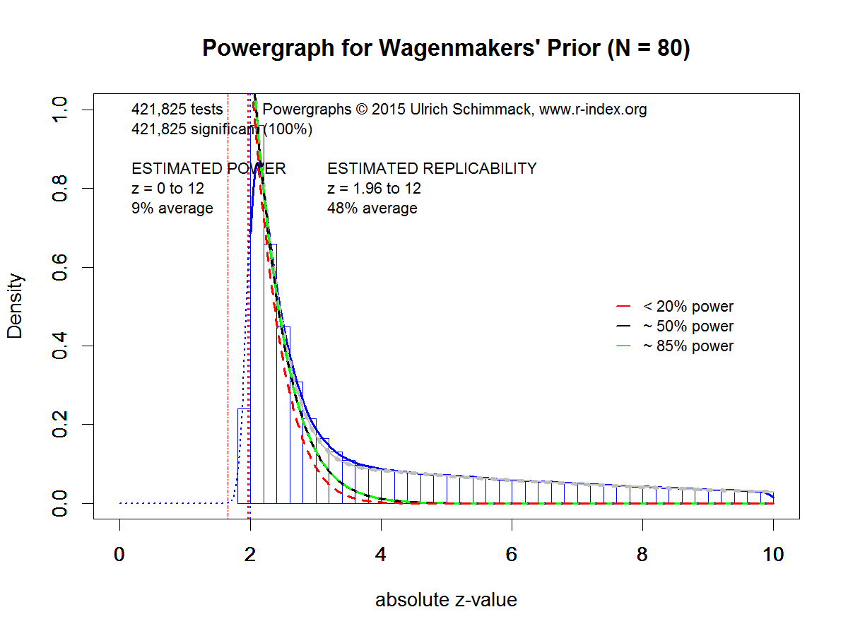
For the simulation I converted the non-central t-values into non-central z-scores and simulated sampling error with a standard normal distribution.  The simulation included 92% true null-hypotheses and 8% true H1 based on Wagenmaker’s prior.  As published results suffer from publication bias, I simulated publication bias by selecting only observed absolute z-scores greater than 1.96, which corresponds to the p < .05 (two-tailed) significance criterion.  The simulated data were submitted to a powergraph analysis that estimates power and replicability based on the distribution of absolute z-scores.

Figure 1 shows the results.   First, the estimation method slightly underestimated the actual replicability of 50% by 2 percentage points.  Despite this slight estimation error, the Figure accurately illustrates the implications of Wagenmakers’ prior for observed distributions of absolute z-scores.  The density function shows a steep decrease in the range of z-scores between 2 and 3, and a gentle slope for z-scores greater than 4 to 10 (values greater than 10 are not shown).

Powergraphs provide some information about the composition of the total density by dividing the total density into densities for power less than 20%, 20-50%, 50% to 85% and more than 85%. The red line (power < 20%) mostly determines the shape of the total density function for z-scores from 2 to 2.5, and most the remaining density is due to studies with more than 85% power starting with z-scores around 4.   Studies with power in the range between 20% and 85% contribute very little to the total density. Thus, the plot correctly reveals that Wagenmakers’ prior assumes that the roughly 50% average replicability is mostly due to studies with very low power (< 20%) and studies with very high power (> 85%).
Powergraph for Wagenmakers' Prior (N = 80)

Validation Study 1: Michael Nujiten’s Statcheck Data

There are a number of datasets that can be used to evaluate Wagenmakers’ prior. The first dataset is based on an automatic extraction of test statistics from psychological journals. I used Michael Nuijten’s dataset to ensure that I did not cheery-pick data and to allow other researchers to reproduce the results.

The main problem with automatically extracted test statistics is that the dataset does not distinguish between  theoretically important test statistics and other statistics, such as significance tests of manipulation checks.  It is also not possible to distinguish between between-subject and within-subject designs.  As a result, replicability estimates for this dataset will be higher than the simulation based on a between-subject design.

Powergraph for Michele Nuijten's StatCheck Data


Figure 2 shows all of the data, but only significant z-scores (z > 1.96) are used to estimate replicability and power. The most striking difference between Figure 1 and Figure 2 is the shape of the total density on the right side of the significance criterion.  In Figure 2 the slope is shallower. The difference is visible in the decomposition of the total density into densities for different power bands.  In Figure 1 most of the total density was accounted for by studies with less than 20% power and studies with more than 85% power.  In Figure 2, studies with power in the range between 20% and 85% account for the majority of studies with z-scores greater than 2.5 up to z-scores of 4.5.

The difference between Figure 1 and Figure 2 has direct implications for the interpretation of Bayes-Factors with t-values that correspond to z-scores in the range of just significant results. Given Wagenmakers’ prior, z-scores in this range mostly represent false-positive results. However, the real dataset suggests that some of these z-scores are the result of underpowered studies and publication bias. That is, in these studies the null-hypothesis is false, but the significant result will not replicate because these studies have low power.

Validation Study 2:  Open Science Collective Articles (Original Results)

The second dataset is based on the Open Science Collective (OSC) replication project.  The project aimed to replicate studies published in three major psychology journals in the year 2008.  The final number of articles that were selected for replication was 99. The project replicated one study per article, but articles often contained multiple studies.  I computed absolute z-scores for theoretically important tests from all studies of these 99 articles.  This analysis produced 294 test statistics that could be converted into absolute z-scores.

Powergraph for OSC Rep.Project Articles (all studies)
Figure 3 shows clear evidence of publication bias.  No sampling distribution can produce the steep increase in tests around the critical value for significance. This selection is not an artifact of my extraction, but an actual feature of published results in psychological journals (Sterling, 1959).

Given the small number of studies, the figure also contains bootstrapped 95% confidence intervals.  The 95% CI for the power estimate shows that the sample is too small to estimate power for all studies, including studies in the proverbial file drawer, based on the subset of studies that were published. However, the replicability estimate of 49% has a reasonably tight confidence interval ranging from 45% to 66%.

The shape of the density distribution in Figure 3 differs from the distribution in Figure 2 in two ways. Initially the slop is steeper in Figure 3, and there is less density in the tail with high z-scores.  Both aspects contribute to the lower estimate of replicability in Figure 3, suggesting that replicabilty of focal hypothesis tests is lower than replicabilty for all statistical tests.

Comparing Figure 3 and Figure 1 shows again that the powergraph based on Wagenmakers’ prior differs from the powergraph for real data. In this case, the discrepancy is even more notable because focal hypothesis tests rarely produce large z-scores (z > 6).

Validation Study 3:  Open Science Collective Articles (Replication Results)

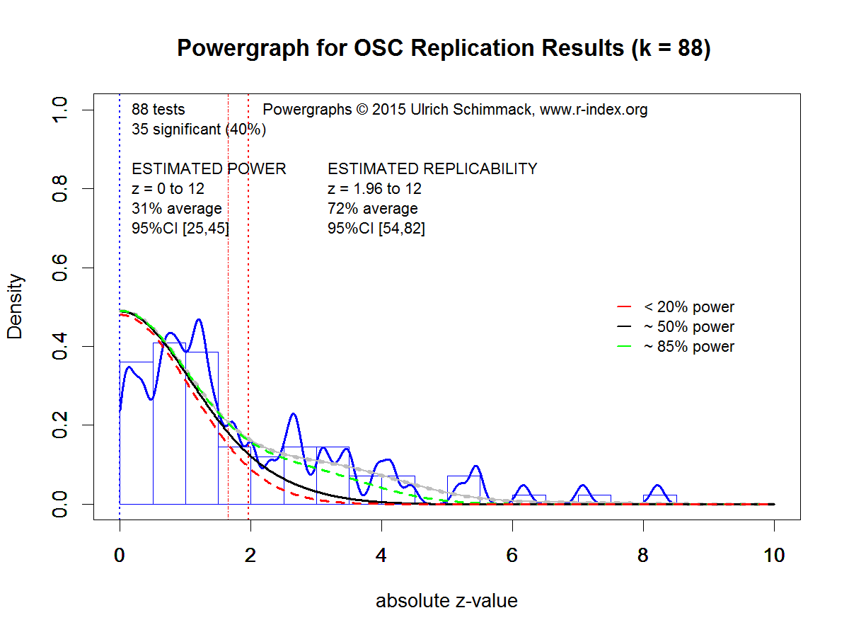
At present, the only data that are somewhat representative of psychological research (at least of social and cognitive psychology) and that do not suffer from publication bias are the results from the replication studies of the OSC replication project.  Out of 97 significant results in original studies, 36 studies (37%) produced that produced a significant result in the original studies produced a significant result in the replication study.  After eliminating some replication studies (e.g., sample of replication study was considerably smaller), 88 studies remained.

Powergraph for OSC Replication Results (k = 88)Figure 4 shows the powergraph for the 88 studies. As there is no publication bias, estimates of power and replicability are based on non-significant and significant results.  Although the sample size is smaller, the estimate of power has a reasonably narrow confidence interval because the estimate includes non-significant results. Estimated power is only 31%. The 95% confidence interval includes the actual success rate of 40%, which shows that there is no evidence of publication bias.
A visual comparison of Figure 1 and Figure 4 shows again that real data diverge from the predicted pattern by Wagenmakers’ prior.  Real data show a greater contribution of power in the range between 20% and 85% to the total density, and large z-scores (z > 6) are relatively rare in real data.

Conclusion

Statisticians have noted that it is good practice to examine the assumptions underlying statistical tests. This blog post critically examines the assumptions underlying the use of Bayes-Factors with Wagenmakers’ prior.  The main finding is that Wagenmaker’s prior makes unreasonable assumptions about power, replicability, and the distribution of observed test-statistics with or without publication bias. The main problem from Wagenmakers’ prior is that it predicts too many statistical results with strong evidence against the null-hypothesis (z > 5, or the 5 sigma rule in physics).  To achieve reasonable predictions for success rates without publication bias (~50%), Wagenmakers’ prior has to assume that over 90% of statistical tests conducted in psychology test false hypothesis (i.e., predict an effect when H0 is true), and that the false-positive rate is close to 50%.

Implications

Bayesian statisticians have pointed out for a long time that the choice of a prior influences Bayes-Factors (Kass, 1993, p. 554).  It is therefore useful to carefully examine priors to assess the effect of priors on Bayesian inferences. Unreasonable priors will lead to unreasonable inferences.  This is also true for Wagenmakers’ prior.

The problem of using Bayes-Factors with Wagenmakers’ prior to test the null-hypothesis is apparent in a realistic scenario that assumes a moderate population effect size of d = .5 and a sample size of N = 80 in a between subject design. This study has a non-central t of 2.24 and 60% power to produce a significant result with p < .05, two-tailed.   I used R to simulate 10,000 test-statistics using the non-central t-distribution and then computed Bayes-Factors with Wagenmakers’ prior.

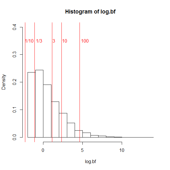
Figure 5 shows a histogram of log(BF). The log is being used because BF are ratios and have very skewed distributions.  The histogram shows that BF never favor the null-hypothesis with a BF of 10 in favor of H0 (1/10 in the histogram).  The reason is that even with Wagenmakers’ prior a sample size of N = 80 is too small to provide strong support for the null-hypothesis.  However, 21% of observed test statistics produce a Bayes-Factor less than 1/3, which is sometimes used as sufficient evidence to claim that the data support the null-hypothesis.  This means that the test has a 21% error rate to provide evidence for the null-hypothesis when the null-hypothesis is false.  A 21% error rate is 4 times larger than the 5% error rate in null-hypothesis significance testing. It is not clear why researchers should replace a statistical method with a 5% error rate for a false discovery of an effect with a 20% error rate of false discoveries of null effects.

Another 48% of the results produce Bayes-Factors that are considered inconclusive. This leaves 31% of results that favor H1 with a Bayes-Factor greater than 3, and only 17% of results produce a Bayes-Factor greater than 10.   This implies that even with the low standard of a BF > 3, the test has only 31% power to provide evidence for an effect that is present.

These results are not wrong because they correctly express the support that the observed data provide for H0 and H1.  The problem only occurs when the specification of H1 is ignored. Given Wagenmakers prior, it is much more likely that a t-value of 1 stems from the sampling distribution of H0 than from the sampling distribution of H1.  However, studies with 50% power when an effect is present are also much more likely to produce t-values of 1 than t-values of 6 or larger.   Thus, a different prior that is more consistent with the actual power of studies in psychology would produce different Bayes-Factors and reduce the percentage of false discoveries of null effects.  Thus, researchers who think Wagenmakers’ prior is not a realistic prior for their research domain should use a more suitable prior for their research domain.

HistogramBF


Counterarguments

Wagenmakers’ has ignored previous criticisms of his prior.  It is therefore not clear what counterarguments he would make.  Below, I raise some potential counterarguments that might be used to defend the use of Wagenmakers’ prior.

One counterargument could be that the prior is not very important because the influence of priors on Bayes-Factors decreases as sample sizes increase.  However, this argument ignores the fact that Bayes-Factors are often used to draw inferences from small samples. In addition, Kass (1993) pointed out that “a simple asymptotic analysis shows that even in large samples Bayes factors remain sensitive to the choice of prior” (p. 555).

Another counterargument could be that a bias in favor of H0 is desirable because it keeps the rate of false-positives low. The problem with this argument is that Bayesian statistics does not provide information about false-positive rates.  Moreover, the cost for reducing false-positives is an increase in the rate of false negatives; that is, either inconclusive results or false evidence for H0 when an effect is actually present.  Finally, the choice of the correct prior will minimize the overall amount of errors.  Thus, it should be desirable for researchers interested in Bayesian statistics to find the most appropriate priors in order to minimize the rate of false inferences.

A third counterargument could be that Wagenmakers’ prior expresses a state of maximum uncertainty, which can be considered a reasonable default when no data are available.  If one considers each study as a unique study, a default prior of maximum uncertainty would be a reasonable starting point.  In contrast, it may be questionable to treat a new study as a randomly drawn study from a sample of studies with different population effect sizes.  However, Wagenmakers’ prior does not express a state of maximum uncertainty and makes assumptions about the probability of observing very large effect sizes.  It does so without any justification for this expectation.  It therefore seems more reasonable to construct priors that are consistent with past studies and to evaluate priors against actual results of studies.

A fourth counterargument is that Bayes-Factors are superior because they can provide evidence for the null-hypothesis and the alternative hypothesis.  However, this is not correct. Bayes-Factors only provide relative support for the null-hypothesis relative to a specific alternative hypothesis.  Researchers who are interested in testing the null-hypothesis can do so using parameter estimation with confidence or credibility intervals. If the interval falls within a specified region around zero, it is possible to affirm the null-hypothesis with a specified level of certainty that is determined by the precision of the study to estimate the population effect size.  Thus, it is not necessary to use Bayes-Factors to test the null-hypothesis.

In conclusion, Bayesian statistics and other statistics are not right or wrong. They combine assumptions and data to draw inferences.  Untrustworthy data and wrong assumptions can lead to false conclusions.  It is therefore important to test the integrity of data (e.g., presence of publication bias) and to examine assumptions.  The uncritical use of Bayes-Factors with default assumptions is not good scientific practice and can lead to false conclusions just like the uncritical use of p-values can lead to false conclusions.

A comparison of The Test of Excessive Significance and the Incredibility Index

A comparison of The Test of Excessive Significance and the Incredibility Index

It has been known for decades that published research articles report too many significant results (Sterling, 1959).  This phenomenon is called publication bias.  Publication bias has many negative effects on scientific progress and undermines the value of meta-analysis as a tool to accumulate evidence from separate original studies.

Not surprisingly, statisticians have tried to develop statistical tests of publication bias.  The most prominent tests are funnel plots (Light & Pillemer, 1984) and Eggert regression (Eggert et al., 1997). Both tests rely on the fact that population effect sizes are statistically independent of sample sizes.  As a result, observed effect sizes in a representative set of studies should also be independent of sample size.  However, publication bias will introduce a negative correlation between observed effect sizes and sample sizes because larger effects are needed in smaller studies to produce a significant result.  The main problem with these bias tests is that other factors may produce heterogeneity in population effect sizes that can also produce variation in observed effect sizes and the variation in population effect sizes may be related to sample sizes.  In fact, one would expect a correlation between population effect sizes and sample sizes if researchers use power analysis to plan their sample sizes.  A power analysis would suggest that researchers use larger samples to study smaller effects and smaller samples to study large effects.  This makes it problematic to draw strong inferences from negative correlations between effect sizes and sample sizes about the presence of publication bias.

Sterling et al. (1995) proposed a test for publication bias that does not have this limitation.  The test is based on the fact that power is defined as the relative frequency of significant results that one would expect from a series of exact replication studies.  If a study has 50% power, the expected frequency of significant results in 100 replication studies is 50 studies.  Publication bias will lead to an inflation in the percentage of significant results. If only significant results are published, the percentage of significant results in journals will be 100%, even if studies had only 50% power to produce significant results.  Sterling et al. (1995) found that several journals reported over 90% of significant results. Based on some conservative estimates of power, he concluded that this high success rate can only be explained with publication bias.  Sterling et al. (1995), however, did not develop a method that would make it possible to estimate power.

Ioannidis and Trikalonis (2007) proposed the first test for publication bias based on power analysis.  They call it “An exploratory test for an excess of significant results.” (ETESR). They do not reference Sterling et al. (1995), suggesting that they independently rediscovered the usefulness of power analysis to examine publication bias.  The main problem for any bias test is to obtain an estimate of (true) power. As power depends on population effect sizes, and population effect sizes are unknown, power can only be estimated.  ETSESR uses a meta-analysis of effect sizes for this purpose.

This approach makes a strong assumption that is clearly stated by Ioannidis and Trikalonis (2007).  The test works well “If it can be safely assumed that the effect is the same in all studies on the same question” (p. 246). In other words, the test may not work well when effect sizes are heterogeneous.  Again, the authors are careful to point out this limitation of ETSER. “In the presence of considerable between-study heterogeneity, efforts should be made first to dissect sources of heterogeneity [33,34]. Applying the test ignoring genuine heterogeneity is ill-advised” (p. 246).

The authors repeat this limitation at the end of the article. “Caution is warranted when there is genuine between-study heterogeneity. Test of publication bias generally yield spurious results in this setting.” (p. 252).   Given these limitations, it would be desirable to develop a test that that does not have to assume that all studies have the same population effect size.

In 2012, I developed the Incredibilty Index (Schimmack, 2012).  The name of the test is based on the observation that it becomes increasingly likely that a set of studies produces a non-significant result as the number of studies increases.  For example, if studies have 50% power (Cohen, 1962), the chance of obtaining a significant result is equivalent to a coin flip.  Most people will immediately recognize that it becomes increasingly unlikely that a fair coin will produce the same outcome again and again and again.  Probability theory shows that this outcome becomes very unlikely even after just a few coin tosses as the cumulative probability decreases exponentially from 50% to 25% to 12.5%, 6.25%, 3.1.25% and so on.  Given standard criteria of improbability (less than 5%), a series of 5 significant results would be incredible and sufficient to be suspicious that the coin is fair, especially if it always falls on the side that benefits the person who is throwing the coin. As Sterling et al. (1995) demonstrated, the coin tends to favor researchers’ hypothesis at least 90% of the time.  Eight studies are sufficient to show that even a success rate of 90% is improbable (p < .05).  It therefore very easy to show that publication bias contributes to the incredible success rate in journals, but it is also possible to do so for smaller sets of studies.

To avoid the requirement of a fixed effect size, the incredibility index computes observed power for individual studies. This approach avoids the need to aggregate effect sizes across studies. The problem with this approach is that observed power of a single study is a very unreliable measure of power (Yuan & Maxwell, 2006).  However, as always, the estimate of power becomes more precise when power estimates of individual studies are combined.  The original incredibility indices used the mean to estimate averaged power, but Yuan and Maxwell (2006) demonstrated that the mean of observed power is a biased estimate of average (true) power.  In further developments of my method, I changed the method and I am now using median observed power (Schimmack, 2016).  The median of observed power is an unbiased estimator of power (Schimmack, 2015).

In conclusion, the Incredibility Index and the Exploratory Test for an Excess of Significant Results are similar tests, but they differ in one important aspect.  ETESR is designed for meta-analysis of highly similar studies with a fixed population effect size.  When this condition is met, ETESR can be used to examine publication bias.  However, when this condition is violated and effect sizes are heterogeneous, the incredibility index is a superior method to examine publication bias. At present, the Incredibility Index is the only test for publication bias that does not assume a fixed population effect size, which makes it the ideal test for publication bias in heterogeneous sets of studies.

References

Light, J., Pillemer, D. B.  (1984). Summing up: The Science of Reviewing Research. Cambridge, Massachusetts.: Harvard University Press.

Egger, M., Smith, G. D., Schneider, M., & Minder, C. (1997). Bias in meta-analysis detected by a simple, graphical test”. BMJ 315 (7109): 629–634. doi:10.1136/bmj.315.7109.629.

Ioannidis and Trikalinos (2007).  An exploratory test for an excess of significant findings. Clinical Trials, 4 245-253.

Schimmack (2012). The Ironic effect of significant results on the credibility of multiple study articles. Psychological Methods, 17, 551-566.

Schimmack, U. (2016). A revised introduction o the R-Index.

Schimmack, U. (2015). Meta-analysis of observed power.

Sterling, T. D. (1959). Publication decisions and their possible effects on inferences drawn from tests of significance: Or vice versa. Journal of the American Statistical Association, 54(285), 30-34. doi: 10.2307/2282137

Stering, T. D., Rosenbaum, W. L., & Weinkam, J. J. (1995). Publication Decisions Revisited: The Effect of the Outcome of Statistical Tests on the Decision to Publish and Vice Versa, The American Statistician, 49, 108-112.

Yuan, K.-H., & Maxwell, S. (2005). On the Post Hoc Power in Testing Mean Differences. Journal of Educational and Behavioral Statistics, 141–167

Replicability Report No. 1: Is Ego-Depletion a Replicable Effect?

Abstract

It has been a common practice in social psychology to publish only significant results.  As a result, success rates in the published literature do not provide empirical evidence for the existence of a phenomenon.  A recent meta-analysis suggested that ego-depletion is a much weaker effect than the published literature suggests and a registered replication study failed to find any evidence for it.  This article presents the results of a replicability analysis of the ego-depletion literature.  Out of 165 articles with 429 studies (total N  = 33,927),  128 (78%) showed evidence of bias and low replicability (Replicability-Index < 50%).  Closer inspection of the top 10 articles with the strongest evidence against the null-hypothesis revealed some questionable statistical analyses, and only a few articles presented replicable results.  The results of this meta-analysis show that most published findings are not replicable and that the existing literature provides no credible evidence for ego-depletion.  The discussion focuses on the need for a change in research practices and suggests a new direction for research on ego-depletion that can produce conclusive results.

INTRODUCTION

In 1998, Roy F. Baumeister and colleagues published a groundbreaking article titled “Ego Depletion: Is the Active Self a Limited Resource?”   The article stimulated research on the newly minted construct of ego-depletion.  At present, more than 150 articles and over 400 studies with more than 30,000 participants have contributed to the literature on ego-depletion.  In 2010, a meta-analysis of nearly 100 articles, 200 studies, and 10,000 participants concluded that ego-depletion is a real phenomenon with a moderate to strong effect size of six tenth of a standard deviation (Hagger et al., 2010).

In 2011, Roy F. Baumeister and John Tierney published a popular book on ego-depletion titled “Will-Power,” and Roy F. Baumeister became to be known as the leading expert on self-regulation, will-power (The Atlantic, 2012).

Everything looked as if ego-depletion research has a bright future, but five years later the future of ego-depletion research looks gloomy and even prominent ego-depletion researchers wonder whether ego-depletion even exists (Slate, “Everything is Crumbling”, 2016).

An influential psychological theory, borne out in hundreds of experiments, may have just been debunked. How can so many scientists have been so wrong?

What Happened?

It has been known for 60 years that scientific journals tend to publish only successful studies (Sterling, 1959).  That is, when Roy F. Baumeister reported his first ego-depletion study and found that resisting the temptation to eat chocolate cookies led to a decrease in persistence on a difficult task by 17 minutes, the results were published as a groundbreaking discovery.  However, when studies do not produce the predicted outcome, they are not published.  This bias is known as publication bias.  Every researcher knows about publication bias, but the practice is so widespread that it is not considered a serious problem.  Surely, researches would not conduct more failed studies than successful studies and only report the successful ones.  Yes, omitting a few studies with weaker effects leads to an inflation of the effect size, but the successful studies still show the general trend.

The publication of one controversial article in the same journal that published the first ego-depletion article challenged this indifferent attitude towards publication bias. In a shocking article, Bem (2011) presented 9 successful studies demonstrating that extraverted students at Cornell University were seemingly able to foresee random events in the future. In Study 1, they seemed to be able to predict where a computer would present an erotic picture even before the computer randomly determined the location of the picture.  Although the article presented 9 successful studies and 1 marginally successful study, researchers were not convinced that extrasensory perception is a real phenomenon.  Rather, they wondered how credible the evidence in other article is if it is possible to get 9 significant results for a phenomenon that few researchers believed to be real.  As Sterling (1959) pointed out, a 100% success rate does not provide evidence for a phenomenon if only successful studies are reported. In this case, the success rate is by definition 100% no matter whether an effect is real or not.

In the same year, Simmons et al. (2011) showed how researchers can increase the chances to get significant results without a real effect by using a number of statistical practices that seem harmless, but in combination can increase the chance of a false discovery by more than 1000% (from 5% to 60%).  The use of these questionable research practices has been compared to the use of doping in sports (John et al., 2012).  Researchers who use QRPs are able to produce many successful studies, but the results of these studies cannot be replicated when other researchers replicate the reported studies without QRPs.  Skeptics wondered whether many discoveries in psychology are as incredible as Bem’s discovery of extrasensory perception; groundbreaking, spectacular, and false.  Is ego-depletion a real effect or is it an artificial product of publication bias and questionable research practices?

Does Ego-Depletion Depend on Blood Glucose?

The core assumption of ego-depletion theory is that working on an effortful task requires energy and that performance decreases as energy levels decrease.  If this theory is correct, it should be possible to find a physiological correlate of this energy.  Ten years after the inception of ego-depletion theory, Baumeister and colleagues claimed to have found the biological basis of ego-depletion in an article called “Self-control relies on glucose as a limited energy source.”  (Gailliot et al., 2007).  The article had a huge impact on ego-depletion researchers and it became a common practice to measure blood-glucose levels.

Unfortunately, Baumeister and colleagues had not consulted with physiological psychologists when they developed the idea that brain processes depend on blood-glucose levels.  To maintain vital functions, the human body ensures that the brain is relatively independent of peripheral processes.  A large literature in physiological psychology suggested that inhibiting the impulse to eat delicious chocolate cookies would not lead to a measurable drop in blood glucose levels (Kurzban, 2011).

Let’s look at the numbers. A well-known statistic is that the brain, while only 2% of body weight, consumes 20% of the body’s energy. That sounds like the brain consumes a lot of calories, but if we assume a 2,400 calorie/day diet – only to make the division really easy – that’s 100 calories per hour on average, 20 of which, then, are being used by the brain. Every three minutes, then, the brain – which includes memory systems, the visual system, working memory, then emotion systems, and so on – consumes one (1) calorie. One. Yes, the brain is a greedy organ, but it’s important to keep its greediness in perspective.

But, maybe experts on physiology were just wrong and Baumeister and colleagues made another groundbreaking discovery.  After all, they presented 9 successful studies that appeared to support the glucose theory of will-power, but 9 successful studies alone provide no evidence because it is not clear how these successful studies were produced.

To answer this question, Schimmack (2012) developed a statistical test that provides information about the credibility of a set of successful studies. Experimental researchers try to hold many factors that can influence the results constant (all studies are done in the same laboratory, glucose is measured the same way, etc.).  However, there are always factors that the experimenter cannot control. These random factors make it difficult to predict the exact outcome of a study even if everything goes well and the theory is right.  To minimize the influence of these random factors, researchers need large samples, but social psychologists often use small samples where random factors can have a large influence on results.  As a result, conducting a study is a gamble and some studies will fail even if the theory is correct.  Moreover, the probability of failure increases with the number of attempts.  You may get away with playing Russian roulette once, but you cannot play forever.  Thus, eventually failed studies are expected and a 100% success rate is a sign that failed studies were simply not reported.  Schimmack (2012) was able to use the reported statistics in Gailliot et al. (2007) to demonstrate that it was very likely that the 100% success rate was only achieved by hiding failed studies or with the help of questionable research practices.

Baumeister was a reviewer of Schimmack’s manuscript and confirmed the finding that a success rate of 9 out of 9 studies was not credible.

 “My paper with Gailliot et al. (2007) is used as an illustration here. Of course, I am quite familiar with the process and history of that one. We initially submitted it with more studies, some of which had weaker results. The editor said to delete those. He wanted the paper shorter so as not to use up a lot of journal space with mediocre results. It worked: the resulting paper is shorter and stronger. Does that count as magic? The studies deleted at the editor’s request are not the only story. I am pretty sure there were other studies that did not work. Let us suppose that our hypotheses were correct and that our research was impeccable. Then several of our studies would have failed, simply given the realities of low power and random fluctuations. Is anyone surprised that those studies were not included in the draft we submitted for publication? If we had included them, certainly the editor and reviewers would have criticized them and formed a more negative impression of the paper. Let us suppose that they still thought the work deserved publication (after all, as I said, we are assuming here that the research was impeccable and the hypotheses correct). Do you think the editor would have wanted to include those studies in the published version?”

To summarize, Baumeister defends the practice of hiding failed studies with the argument that this practice is acceptable if the theory is correct.  But we do not know whether the theory is correct without looking at unbiased evidence.  Thus, his line of reasoning does not justify the practice of selectively reporting successful results, which provides biased evidence for the theory.  If we could know whether a theory is correct without data, we would not need empirical tests of the theory.  In conclusion, Baumeister’s response shows a fundamental misunderstanding of the role of empirical data in science.  Empirical results are not mere illustrations of what could happen if a theory were correct. Empirical data are supposed to provide objective evidence that a theory needs to explain.

Since my article has been published, there have been several failures to replicate Gailliot et al.’s findings and recent theoretical articles on ego-depletion no longer assume that blood-glucose as the source of ego-depletion.

“Upon closer inspection notable limitations have emerged. Chief among these is the failure to replicate evidence that cognitive exertion actually lowers blood glucose levels.” (Inzlicht, Schmeichel, & Macrae, 2014, p 18).

Thus, the 9 successful studies that were selected by Baumeister et al. (1998) did not illustrate an empirical fact, they created false evidence for a physiological correlate of ego-depletion that could not be replicated.  Precious research resources were wasted on a line of research that could have been avoided by consulting with experts on human physiology and by honestly examining the successful and failed studies that led to the Baumeister et al. (1998) article.

Even Baumeister agrees that the original evidence was false and that glucose is not the biological correlate of ego-depletion.

In retrospect, even the initial evidence might have gotten a boost in significance from a fortuitous control condition. Hence at present it seems unlikely that ego depletion’s effects are caused by a shortage of glucose in the bloodstream” (Baumeister, 2014, p 315).

Baumeister fails to mention that the initial evidence also got a boost from selection bias.

In sum, the glucose theory of ego-depletion was based on selective reporting of studies that provided misleading support for the theory and the theory lacks credible empirical support.  The failure of the glucose theory raises questions about the basic ego-depletion effect.  If researchers in this field used selective reporting and questionable research practices, the evidence for the basic effect is also likely to be biased and the effect may be difficult to replicate.

If 200 studies show ego-depletion effects, it must be real?

Psychologists have not ignored publication bias altogether.  The main solution to the problem is to conduct meta-analyses.  A meta-analysis combines information from several small studies to examine whether an effect is real.  The problem for meta-analysis is that publication bias also influences the results of a meta-analysis.  If only successful studies are published, a meta-analysis of published studies will show evidence for an effect no matter whether the effect actually exists or not.  For example, the top journal for meta-analysis, Psychological Bulletin, has published meta-analyses that provide evidence for extransensory perception (Bem & Honorton, 1994).

To address this problem, meta-analysts have developed a number of statistical tools to detect publication bias.  The most prominent method is Eggert’s regression of effect size estimates on sampling error.  A positive correlation can reveal publication bias because studies with larger sampling errors (small samples) require larger effect sizes to achieve statistical significance.  To produce these large effect sizes when the actual effect does not exist or is smaller, researchers need to hide more studies or use more questionable research practices.  As a result, these results are particularly difficult to replicate.

Although the use of these statistical methods is state of the art, the original ego-depletion meta-analysis that showed moderate to large effects did not examine the presence of publication bias (Hagger et al., 2010). This omission was corrected in a meta-analysis by Carter and McCollough (2014).

Upon reading Hagger et al. (2010), we realized that their efforts to estimate and account for the possible influence of publication bias and other small-study effects had been less than ideal, given the methods available at the time of its publication (Carter & McCollough, 2014).

The authors then used Eggert regression to examine publication bias.  Moreover, they used a new method that was not available at the time of Hagger et al.’s (2010) meta-analysis to estimate the effect size of ego-depletion after correcting for the inflation caused by publication bias.

Not surprisingly, the regression analysis showed clear evidence of publication bias.  More stunning were the results of the effect size estimate after correcting for publication bias.  The bias-corrected effect size estimate was d = .25 with a 95% confidence interval ranging from d = .18 to d = .32.   Thus, even the upper limit of the confidence interval is about 50% less than the effect size estimate in the original meta-analysis without correction for publication bias.   This suggests that publication bias inflated the effect size estimate by 100% or more.  Interestingly, a similar result was obtained in the reproducibility project, where a team of psychologists replicated 100 original studies and found that published effect sizes were over 100% larger than effect sizes in the replication project (OSC, 2015).

An effect size of d = .2 is considered small.  This does not mean that the effect has no practical importance, but it raises questions about the replicability of ego-depletion results.  To obtain replicable results, researchers should plan studies so that they have an 80% chance to get significant results despite the unpredictable influence of random error.  For small effects, this implies that studies require large samples.  For the standard ego-depletion paradigm with an experimental group and a control group and an effect size of d = .2, a sample size of 788 participants is needed to achieve 80% power. However, the largest sample size in an ego-depletion study was only 501 participants.  A sample size of 388 participants is needed to achieve significance without an inflated effect size (50% power) and most studies fall short of this requirement in sample size.  Thus, most published ego-depletion results are unlikely to replicate and future ego-depletion studies are likely to produce non-significant results.

In conclusion, even 100 studies with 100% successful results do not provide convincing evidence that ego-depletion exists and which experimental procedures can be used to replicate the basic effect.

Replicability without Publication Bias

In response to concerns about replicability, the American Psychological Society created a new format for publications.  A team of researchers can propose a replication project.  The research proposal is peer-reviewed like a grant application.  When the project is approved, researchers conduct the studies and publish the results independent of the outcome of the project.  If it is successful, the results confirm that earlier findings that were reported with publication bias are replicable, although probably with a smaller effect size.  If the studies fail, the results suggest that the effect may not exist or that the effect size is very small.

In the fall of 2014 Hagger and Chatzisarantis announced a replication project of an ego-depletion study.

The third RRR will do so using the paradigm developed and published by Sripada, Kessler, and Jonides (2014), which is similar to that used in the original depletion experiments (Baumeister et al., 1998; Muraven et al., 1998), using only computerized versions of tasks to minimize variability across laboratories. By using preregistered replications across multiple laboratories, this RRR will allow for a precise, objective estimate of the size of the ego depletion effect.

In the end, 23 laboratories participated and the combined sample size of all studies was N = 2141.  This sample size affords an 80% probability to obtain a significant result (p < .05, two-tailed) with an effect size of d = .12, which is below the lower limit of the confidence interval of the bias-corrected meta-analysis.  Nevertheless, the study failed to produce a statistically significant result, d = .04 with a 95%CI ranging from d = -.07 to d = .14.  Thus, the results are inconsistent with a small effect size of d = .20 and suggest that ego-depletion may not even exist at all.

Ego-depletion researchers have responded to this result differently.  Michael Inzlicht, winner of a theoretical innovation prize for his work on ego-depletion, wrote:

The results of a massive replication effort, involving 24 labs (or 23, depending on how you count) and over 2,000 participants, indicates that short bouts of effortful control had no discernable effects on low-level inhibitory control. This seems to contradict two decades of research on the concept of ego depletion and the resource model of self-control. Like I said: science is brutal.

In contrast, Roy F. Baumeister questioned the outcome of this research project that provided the most comprehensive and scientific test of ego-depletion.  In a response with co-author Kathleen D. Vohs titled “A misguided effort with elusive implications,” Baumeister tries to explain why ego depletion is a real effect, despite the lack of unbiased evidence for it.

The first line of defense is to question the validity of the paradigm that was used for the replication project. The only problem is that this paradigm seemed reasonable to the editors who approved the project, researchers who participated in the project and who expected a positive result, and to Baumeister himself when he was consulted during the planning of the replication project.  In his response, Baumeister reverses his opinion about the paradigm.

In retrospect, the decision to use new, mostly untested procedures for a large replication project was foolish.

He further claims that he proposed several well-tested procedures, but that these procedures were rejected by the replication team for technical reasons.

Baumeister nominated several procedures that have been used in successful studies of ego depletion for years. But none of Baumeister’s suggestions were allowable due to the RRR restrictions that it must be done with only computerized tasks that were culturally and linguistically neutral.

Baumeister and Vohs then claim that the manipulation did not lead to ego-depletion and that it is not surprising that an unsuccessful manipulation does not produce an effect.

Signs indicate the RRR was plagued by manipulation failure — and therefore did not test ego depletion.

They then assure readers that ego-depletion is real because they have demonstrated the effect repeatedly using various experimental tasks.

For two decades we have conducted studies of ego depletion carefully and honestly, following the field’s best practices, and we find the effect over and over (as have many others in fields as far-ranging as finance to health to sports, both in the lab and large-scale field studies). There is too much evidence to dismiss based on the RRR, which after all is ultimately a single study — especially if the manipulation failed to create ego depletion.

This last statement is, however, misleading if not outright deceptive.  As noted earlier, Baumeister admitted to the practice of not publishing disconfirming evidence.  He and I disagree whether the selective publication of successful studies is honest or dishonest.  He wrote:

 “We did run multiple studies, some of which did not work, and some of which worked better than others. You may think that not reporting the less successful studies is wrong, but that is how the field works.” (Roy Baumeister, personal email communication)

So, when Baumeister and Vohs assure readers that they conducted ego-depletion research carefully and honestly, they are not saying that they reported all studies that they conducted in their labs.  The successful studies published in articles are not representative of the studies conducted in their labs.

In a response to Baumeister and Vohs, the lead authors of the replication project pointed out that ego-depletion does not exist unless proponents of ego-depletion theory can specify experimental procedures that reliably produce the predicted effect.

The onus is on researchers to develop a clear set of paradigms that reliably evoke depletion in large samples with high power (Hagger & Chatzisarantis, 2016)

In an open email letter, I asked Baumeister and Vohs to name paradigms that could replicate a published ego-depletion effect.  They were not able or willing to name a single paradigm. Roy Bameister’s response was “In view of your reputation as untrustworthy, dishonest, and otherwise obnoxious, i prefer not to cooperate or collaborate with you.” 

I did not request to collaborate with him.  I merely asked which paradigm would be able to produce ego-depletion effects in an open and transparent replication study, given his criticism of the most rigorous replication study that he initially approved.

If an expert who invented a theory and published numerous successful studies cannot name a paradigm that will work, it suggests that he does not know which studies may work because for each published successful study there are unpublished, unsuccessful studies that used the same procedure, and it is not obvious which study would actually replicate in an honest and transparent replication project.

A New Meta-Analysis of Ego-Depletion Studies:  Are there replicable effects?

Since I published the incredibility index (Schimmack, 2012) and demonstrated bias in research on glucose and ego-depletion, I have developed new and more powerful ways to reveal selection bias and questionable research practices.  I applied these methods to the large literature on ego-depletion to examine whether there are some credible ego-depletion effects and a paradigm that produces replicable effects.

The first method uses powergraphs (Schimmack, 2015) to examine selection bias and the replicability of a set of studies. To create a powergrpah, original research results are converted into absolute z-score.  A z-score shows how much evidence a study result provides against the null-hypothesis that there is no effect.  Unlike effect size measures, z-scores also contain information about the sample size (sampling error).   I therefore distinguish between meta-analysis of effect sizes and meta-analysis of evidence.  Effect size meta-analysis aims to determine the typical, average size of an effect.  Meta-analyses of evidence examine how strong the evidence for an effect (i.e., against the null-hypothesis of no effect) is.

The distribution of absolute z-scores provides important information about selection bias, questionable research practices, and replicability.  Selection bias is revealed if the distribution of z-scores shows a steep drop on the left side of the criterion for statistical significance (this is analogous to the empty space below the line for significance in a funnel plot). Questionable research practices are revealed if z-scores cluster in the area just above the significance criterion.  Replicabilty is estimated by fitting a weighted composite of several non-central distributions that simulate studies with different non-centrality parameters and sampling error.

A literature search retrieved 165 articles that reported 429 studies.  For each study, the most important statistical test was converted first into a two-tailed p-value and then into a z-score.  A single test statistic was used to ensure that all z-scores are statistically independent.

Powergraph for Ego Depletion (Focal Tests)


The results show clear evidence of selection bias (Figure 1).  Although there are some results below the significance criterion (z = 1.96, p < .05, two-tailed), most of these results are above z = 1.65, which corresponds to p < .10 (two-tailed) or p < .05 (one-tailed).  These results are typically reported as marginally significant and used as evidence for an effect.   There are hardly any results that fail to confirm a prediction based on ego-depletion theory.  Using z = 1.65 as criterion, the success rate is 96%, which is common for the reported success rate in psychological journals (Sterling, 1959; Sterling et al., 1995; OSC, 2015).  The steep cliff in the powergraph shows that this success rate is due to selection bias because random error would have produced a more gradual decline with many more non-significant results.

The next observation is the tall bar just above the significance criterion with z-scores between 2 and 2.2.   This result is most likely due to questionable research practices that lead to just significant results such as optional stopping or selective dropping of outliers.

Another steep drop is observed at z-scores of 2.6.  This drop is likely due to the use of further questionable research practices such as dropping of experimental conditions, use of multiple dependent variables, or simply running multiple studies and selecting only significant results.

A rather large proportion of z-scores are in the questionable range from z = 1.96 to 2.60.  These results are unlikely to replicate. Although some studies may have reported honest results, there are too many questionable results and it is impossible to say which results are trustworthy and which results are not.  It is like getting information from a group of people where 60% are liars and 40% tell the truth.  Even though 40% are telling the truth, the information is useless without knowing who is telling the truth and who is lying.

The best bet to find replicable ego-depletion results is to focus on the largest z-scores as replicability increases with the strength of evidence (OSC, 2015). The power estimation method uses the distribution of z-scores greater than 2.6 to estimate the average power of these studies.  The estimated power is 47% with a 95% confidence interval ranging from 32% to 63%.  This result suggests that some ego-depletion studies have produced replicable results.  In the next section, I examine which studies this may be.

In sum, a state-of-the art meta-analysis of evidence for an effect in the ego-depletion literature shows clear evidence for selection bias and the use of questionable research practices.  Many published results are essentially useless because the evidence is not credible.  However, the results also show that some studies produced replicable effects, which is consistent with Carter and McCollough’s finding that the average effect size is likely to be above zero.

What Ego-Depletion Studies Are Most Likely to Replicate?

Powergraphs are useful for large sets of heterogeneous studies.  However, they are not useful to examine the replicability of a single study or small sets of studies, such as a set of studies in a multiple-study article.  For this purpose, I developed two additional tools that detect bias in published results. .

The Test of Insufficient Variance (TIVA) requires a minimum of two independent studies.  As z-scores follow a normal distribution (the normal distribution of random error), the variance of z-scores should be 1.  However, if non-significant results are omitted from reported results, the variance shrinks.  TIVA uses the standard comparison of variances to compute the probability that an observed variance of z-scores is an unbiased sample drawn from a normal distribution.  TIVA has been shown to reveal selection bias in Bem’s (2011) article and it is a more powerful test than the incredibility index (Schimmack, 2012).

The R-Index is based on the Incredibilty Index in that it compares the success rate (percentage of significant results) with the observed statistical power of a test. However, the R-Index does not test the probability of the success rate.  Rather, it uses the observed power to predict replicability of an exact replication study.  The R-Index has two components. The first component is the median observed power of a set of studies.  In the limit, median observed power approaches the average power of an unbiased set of exact replication studies.  However, when selection bias is present, median observed power is biased and provides an inflated estimate of true power.  The R-Index measures the extent of selection bias by means of the difference between success rate and median observed power.  If median observed power is 75% and the success rate is 100%, the inflation rate is 25% (100 – 75 = 25).  The inflation rate is subtracted from median observed power to correct for the inflation.  The resulting replication index is not directly an estimate of power, except for the special case when power is 50% and the success rate is 100%   When power is 50% and the success rate is 100%, median observed power increases to 75%.  In this case, the inflation correction of 25% returns the actual power of 50%.

I emphasize this special case because 50% power is also a critical point at which point a rational bet would change from betting against replication (Replicability < 50%) to betting on a successful replication (Replicability > 50%).  Thus, an R-Index of 50% suggests that a study or a set of studies produced a replicable result.  With success rates close to 100%, this criterion implies that median observed power is 75%, which corresponds to a z-score of 2.63.  Incidentally, a z-score of 2.6 also separated questionable results from more credible results in the powergraph analysis above.

It may seem problematic to use the R-Index even for a single study because observed power of a single study is strongly influenced by random factors and observed power is by definition above 50% for a significant result. However, The R-Index provides a correction for selection bias and a significant result implies a 100% success rate.  Of course, it could also be an honestly reported result, but if the study was published in a field with evidence of selection bias, the R-Index provides a reasonable correction for publication bias.  To achieve an R-Index above 50%, observed power has to be greater than 75%.

This criterion has been validated with social psychology studies in the reproducibilty project, where the R-Index predicted replication success with over 90% accuracy. This criterion also correctly predicted that the ego-depletion replication project would produce fewer than 50% successful replications, which it did, because the R-Index for the original study was way below 50% (F(1,90) = 4.64, p = .034, z = 2.12, OP = .56, R-Index = .12).  If this information had been available during the planning of the RRR, researchers might have opted for a paradigm with a higher chance of a successful replication.

To identify paradigms with higher replicability, I computed the R-Index and TIVA (for articles with more than one study) for all 165 articles in the meta-analysis.  For TIVA I used p < .10 as criterion for bias and for the R-Index I used .50 as the criterion.   37 articles (22%) passed this test.  This implies that 128 (78%) showed signs of statistical bias and/or low replicability.  Below I discuss the Top 10 articles with the highest R-Index to identify paradigms that may produce a reliable ego-depletion effect.

1. Robert D. Dvorak and Jeffrey S. Simons (PSPB, 2009) [ID = 142, R-Index > .99]

This article reported a single study with an unusually large sample size for ego-depletion studies. 180 participants were randomly assigned to a standard ego-depletion manipulation. In the control condition, participants watched an amusing video.  In the depletion condition, participants watched the same video, but they were instructed to suppress all feelings and expressions.  The dependent variable was persistence on a set of solvable and unsolvable anagrams.  The t-value in this study suggests strong evidence for an ego-depletion effect, t(178) = 5.91.  The large sample size contributes to this, but the effect size is also large, d = .88.

Interestingly, this study is an exact replication of Study 3 in the seminal ego-depletion article by Baumeister et al. (1998), which obtained a significant effect with just 30 participants and a strong effect size of d = .77, t(28) = 2.12.

The same effect was also reported in a study with 132 smokers (Heckman, Ditre, & Brandon, 2012). Smokers who were not allowed to smoke persisted longer on a figure tracing task when they could watch an emotional video normally than when they had to suppress emotional responses, t(64) = 3.15, d = .78.  The depletion effect was weaker when smokers were allowed to smoke between the video and the figure tracing task. The interaction effect was significant, F(1, 128) = 7.18.

In sum, a set of studies suggests that emotion suppression influences persistence on a subsequent task.  The existing evidence suggests that this is a rather strong effect that can be replicated across laboratories.

2. Megan Oaten, Kipling D. William, Andrew Jones, & Lisa Zadro (J Soc Clinical Psy, 2008) [ID = 118, R-Index > .99]

This article reports two studies that manipulated social exclusion (ostracism) under the assumption that social exclusion is ego-depleting. The dependent variable was consumption of an unhealthy food in Study 1 and drinking a healthy, but unpleasant drink in Study 2.  Both studies showed extremely strong effects of ego-depletion (Study 1: d = 2.69, t(71) = 11.48;  Study 2: d = 1.48, t(72) = 6.37.

One concern about these unusually strong effects is the transformation of the dependent variable.  The authors report that they first ranked the data and then assigned z-scores corresponding to the estimated cumulative proportion.  This is an unusual procedure and it is difficult to say whether this procedure inadvertently inflated the effect size of ego-depletion.

Interestingly, one other article used social exclusion as an ego-depletion manipulation (Baumeister et al., 2005).  This article reported six studies and TIVA showed evidence of selection bias, Var(z) = 0.15, p = .02.  Thus, the reported effect sizes in this article are likely to be inflated.  The first two studies used consumption of an unpleasant tasting drink and eating cookies, respectively, as dependent variables. The reported effect sizes were weaker than in the article by Oaten et al. (d = 1.00, d = .90).

In conclusion, there is some evidence that participants avoid displeasure and seek pleasure after social rejection. A replication study with a sufficient sample size may replicate this result with a weaker effect size.  However, even if this effect exists it is not clear that the effect is mediated by ego-depletion.

3. Kathleen D. Vohs & Ronald J. Farber (Journal of Consumer Research) [ID = 29, R-Index > .99]

This article examined the effect of several ego-depletion manipulations on purchasing behavior.  Study 1 found a weaker effect, t(33) = 2.83,  than Studies 2 and 3, t(63) = 5.26, t(33) = 5.52, respectively.  One possible explanation is that the latter studies used actual purchasing behavior.  Study 2 used the White Bear paradigm and Study 2 used amplification of emotion expressions as ego-depletion manipulations.  Although statistically robust, purchasing behavior does not seem to be the best indicator of ego-depletion.  Thus, replication efforts may focus on other dependent variables that measure ego-depletion more directly.

4. Kathleen D. Vohs, Roy F. Baumeister, & Brandon J. Schmeichel (JESP, 2012/2013) [ID = 49, R-Index = .96]

This article was first published in 2012, but the results for Study 1 were misreported and a corrected version was published in 2013.  The article presents two studies with a 2 x 3 between-subject design. Study 1 had n = 13 participants per cell and Study 2 had n = 35 participants per cell.  Both studies showed an interaction between ego-depletion manipulations and manipulations of self-control beliefs. The dependent variables in both studies were the Cognitive Estimation Test and a delay of gratification task.  Results were similar for both dependent measures. I focus on the CET because it provides a more direct test of ego-depletion; that is, the draining of resources.

In the condition with limited-will-power beliefs of Study 1, the standard ego-depletion effect that compares depleted participants to a control condition was a decreased by about 6 points from about 30 to 24 points (no exact means or standard deviations, or t-values for this contrast are provided).  The unlimited will-power condition shows a smaller decrease by 2 points (31 vs. 29).  Study 2 replicates this pattern. In the limited-will-power condition, CET scores decreased again by 6 points from 32 to 26 and in the unlimited-will-power condition CET scores decreased by about 2 points from about 31 to 29 points.  This interaction effect would again suggest that the standard depletion effect can be reduced by manipulating participants’ beliefs.

One interesting aspect of the study was the demonstration that ego-depletion effects increase with the number of ego-depleting tasks.  Performance on the CET decreased further when participants completed 4 vs. 2 or 3 vs. 1 depleting task.  Thus, given the uncertainty about the existence of ego-depletion, it would make sense to start with a strong manipulation that compares a control condition with a condition with multiple ego-depleting tasks.

One concern about this article is the use of the CET as a measure of ego-depletion.  The task was used in only one other study by Schmeichel, Vohs, and Baumeister (2003) with a small sample of N = 37 participants.  The authors reported a just significant effect on the CET, t(35) = 2.18.  However, Vohs et al. (2013) increased the number of items from 8 to 20, which makes the measure more reliable and sensitive to experimental manipulations.

Another limitation of this study is that there was no control condition without manipulation of beliefs. It is possible that the depletion effect in this study was amplified by the limited-will-power manipulation. Thus, a simple replication of this study would not provide clear evidence for ego-depletion.  However, it would be interesting to do a replication study that examines the effect of ego-depletion on the CET without manipulation of beliefs.

In sum, this study could provide the basis for a successful demonstration of ego-depletion by comparing effects on the CET for a control condition versus a condition with multiple ego-depletion tasks.

5. Veronika Job, Carol S. Dweck, and Gregory M. Walton (Psy Science, 2010) [ID = 191, R-Index = 94]

The article by Job et al. (2010) is noteworthy for several reasons.  First, the article presented three close replications of the same effect with high t-values, ts = 3.88, 8.47, 2.62.  Based on these results, one would expect that other researchers can replicate the results.  Second, the effect is an interaction between a depletion manipulation and a subtle manipulation of theories about the effect of working on an effortful task.  Hidden among other questionnaires, participants received either items that suggested depletion (“After a strenuous mental activity your energy is depleted and you must rest to get it refueled again” or items that suggested energy is unlimited (“Your mental stamina fuels itself; even after strenuous mental exertion you can continue doing more of it”). The pattern of the interaction effect showed that only participants who received the depletion items showed the depletion effect.  Participants who received the unlimited energy items showed no significant difference in Stroop performance.  Taken at face value, this finding would challenge depletion theory, which assumes that depletion is an involuntary response to exerting effort.

However, the study also raises questions because the authors used an unconventional statistical method to analyze their data.  Data were analyzed with a multi-level model that modeled errors as a function of factors that vary within participants over time and factors that vary between participants, including the experimental manipulations.  In an email exchange, the lead author confirmed that the model did not include random factors for between-subject variance.  A statistician assured the lead author that this was acceptable.  However, a simple computation of the standard deviation around mean accuracy levels would show that this variance is not zero.  Thus, the model artificially inflated the evidence for an effect by treating between-subject variance as within-subject variance. In a betwee-subject analysis, the small differences in error rates (about 5 percentage points) are unlikely to be significant.

In sum, it is doubtful that a replication study would replicate the interaction between depletion manipulations and the implicit theory manipulation reported in Job et al. (2010) in an appropriate between-subject analysis.  Even if this result would replicate, it would not support the theory that ego-depletion is a limited resource that is depleted after a short effortful task because the effect can be undone with a simple manipulations of beliefs in unlimited energy.

6. Roland Imhoff, Alexander F. Schmidt, & Friederike Gerstenberg (Journal of Personality, 2014) [ID = 146, R-Index = .90]

Study 1 reports results a standard ego-depletion paradigm with a relatively larger sample (N = 123).  The ego-depletion manipulation was a Stroop task with 180 trials.  The dependent variable was consumption of chocolates (M&M).  The study reported a large effect, d = .72, and strong evidence for an ego-depletion effect, t(127) = 4.07.  The strong evidence is in part justified by the large sample size, but the standardized effect size seems a bit large for a difference of 2g in consumption, whereas the standard deviation of consumption appears a bit small (3g).  A similar study with M&M consumption as dependent variable found a 2g difference in the opposite direction with a much larger standard deviation of 16g and no significant effect, t(48) = -0.44.

The second study produced results in line with other ego-depletion studies and did not contribute to the high R-Index of the article, t(101) = 2.59. The third study was a correlational study with examined correlates of a trait measure of ego-depletion.  Even if this correlation is replicable, it does not support the fundamental assumption of ego-depletion theory of situational effects of effort on subsequent effort.  In sum, it is unlikely that Study 1 is replicable and that strong results are due to misreported standard deviations.

7. Hugo J.E.M. Alberts, Carolien Martijn, & Nanne K. de Vries (JESP, 2011) [ID = 56, R-Index = .86]

This article reports the results of a single study that crossed an ego-depletion manipulation with a self-awareness priming manipulation (2 x 2 with n = 20 per cell).  The dependent variable was persistence in a hand-grip task.  Like many other handgrip studies, this study assessed handgrip persistence before and after the manipulation, which increases the statistical power to detect depletion effects.

The study found weak evidence for an ego-depletion effect, but relatively strong evidence for an interaction effect, F(1,71) = 13.00.  The conditions without priming showed a weak ego depletion effect (6s difference, d = .25).  The strong interaction effect was due to the priming conditions, where depleted participants showed an increase in persistence by 10s and participants in the control condition showed a decrease in performance by 15s.  Even if this is a replicable finding, it does not support the ego-depletion effect.  The weak evidence for ego depletion with the handgrip task is consistent with a meta-analysis of handgrip studies (Schimmack, 2015).

In short, although this study produced an R-Index above .50, closer inspection of the results shows no strong evidence for ego-depletion.

8. James M. Tyler (Human Communications Research, 2008) [ID = 131, R-Index = .82]

This article reports three studies that show depletion effects after sharing intimate information with strangers.  In the depletion condition, participants were asked to answer 10 private questions in a staged video session that suggested several other people were listening.  This manipulation had strong effects on persistence in an anagram task (Study 1, d = 1.6, F(2,45) = 16.73) and the hand-grip task (Study 2: d = 1.35, F(2,40) = 11.09). Study 3 reversed tasks and showed that the crossing-E task influenced identification of complex non-verbal cues, but not simple non-verbal cues, F(1,24) = 13.44. The effect of the depletion manipulation on complex cues was very large, d = 1.93.  Study 4 crossed the social manipulation of depletion from Studies 1 and 2 with the White Bear suppression manipulation and used identification of non-verbal cues as the dependent variable.  The study showed strong evidence for an interaction effect, F(1,52) = 19.41.  The pattern of this interaction is surprising, because the White Bear suppression task showed no significant effect after not sharing intimate details, t(28) = 1.27, d = .46.  In contrast, the crossing-E task had produced a very strong effect in Study 3, d = 1.93.  The interaction was driven by a strong effect of the White Bear manipulation after sharing intimate details, t(28) = 4.62, d = 1.69.

Even though the statistical results suggest that these results are highly replicable, the small sample sizes and very large effect sizes raise some concerns about replicability.  The large effects cannot be attributed to the ego-depletion tasks or measures that have been used in many other studies that produced much weaker effect. Thus, the only theoretical explanation for these large effect sizes would be that ego depletion has particularly strong effects on social processes.  Even if these effects could be replicated, it is not clear that ego-depletion is the mediating mechanism.  Especially the complex manipulation in the first two studies allow for multiple causal pathways.  It may also be difficult to recreate this manipulation and a failure to replicate the results could be attribute to problems with reproducibility.  Thus, a replication of this study is unlikely to advance understanding of ego-depletion without first establishing that ego-depletion exists.

9. Brandon J. Schmeichel, Heath A. Demaree, Jennifer L. Robinson, & Jie Pu (Social Cognition, 2006) [ID = 52, R-Index = .80]

This article reported one study with an emotion regulation task. Participants in the depletion condition were instructed to exaggerated emotional responses to a disgusting film clip.  The study used two task to measure ego-depletion.  One task required generation of words; the other task required generation of figures.  The article reports strong evidence in an ANOVA with both dependent variables, F(1,46) = 11.99.  Separate analyses of the means show a stronger effect for the figural task, d = .98, than for the verbal task, d = .50.

The main concern with this study is that the fluency measures were never used in any other study.  If a replication study fails, one could argue that the task is not a valid measure of ego-depletion.  However, the study shows the advantage of using multiple measures to increase statistical power (Schimmack, 2012).

10. Mark Muraven, Marylene Gagne, and Heather Rosman (JESP, 2008) [ID = 15, R-Index = .78]

Study 1 reports the results of a 2 x 2 design with N = 30 participants (~ 7.5 participants per condition).  It crossed an ego-depletion manipulation (resist eating chocolate cookies vs. radishes) with a self-affirmation manipulation.  The dependent variable was the number of errors in a vigilance task (respond to a 4 after a 6).  The results section shows some inconsistencies.  The 2 x 2 ANOVA shows strong evidence for an interaction, F(1,28) = 10.60, but the planned contrast that matches the pattern of means, shows a just significant effect, F(1,28) = 5.18.  Neither of these statistics is consistent with the reported means and standard deviations, where the depleted not affirmed group has twice the number of errors (M = 12.25, SD = 1.63) than the depleted group with affirmation (M = 5.40, SD = 1.34). These results would imply a standardized effect size of d = 4.59.

Study 2 did not manipulate ego-depletion and reported a more reasonable, but also less impressive result for the self-affirmation manipulation, F(2,63) = 4.67.

Study 3 crossed an ego-depletion manipulation with a pressure manipulation.  The ego-depletion task was a computerized ego-depletion task where participants in the depletion condition had to type a paragraph without copying the letter E or spaces. This is more difficult than just copying a paragraph.  The pressure manipulation were constant reminders to avoid making errors and to be as fast as possible.  The sample size was N = 96 (n = 24 per cell).  The dependent variable was the vigilance task from Study 1.  The evidence for a depletion effect was strong, F(1, 92) = 10.72 (z = 3.17).  However, the effect was qualified by the pressure manipulation, F(1,92) = 6.72.  There was a strong depletion effect in the pressure condition, d = .78, t(46) = 2.63, but there was no evidence for a depletion effect in the no-pressure condition, d = -.23, t(46) = 0.78.

The standard deviations in Study 3 that used the same dependent variable were considerable wider than the standard deviations in Study 1, which explains the larger standardized effect sizes in Study 1.  With the standard deviations of Study 3, Study 1 would not have

DISCUSSION AND FUTURE DIRECTIONS

The original ego-depletion article published in 1998 has spawned a large literature with over 150 articles, more than 400 studies, and a total number of over 30,000 participants. There have been numerous theoretical articles and meta-analyses of this literature.  Unfortunately, the empirical results reported in this literature are not credible because there is strong evidence that reported results are biased.  The bias makes it difficult to predict which effects are replicable. The main conclusion that can be drawn from this shaky mountain of evidence is that ego-depletion researchers have to change the way they conduct and report their findings.

Importantly, this conclusion is in stark disagreement with Baumeister’s recommendations.  In a forthcoming article, he suggests that “the field has done very well with the methods and standards it has developed over recent decades,” (p. 2), and he proposes that “we should continue with business as usual” (p. 1).

Baumeister then explicitly defends the practice of selectively publishing studies that produced significant results without reporting failures to demonstrate the effect in conceptually similar studies.

Critics of the practice of running a series of small studies seem to think researchers are simply conducting multiple tests of the same hypothesis, and so they argue that it would be better to conduct one large test. Perhaps they have a point: One big study could be arguably better than a series of small ones. But they also miss the crucial point that the series of small studies is typically designed to elaborate the idea in different directions, such as by identifying boundary conditions, mediators, moderators, and extensions. The typical Study 4 is not simply another test of the same hypothesis as in Studies 1–3. Rather, each one is different. And yes, I suspect the published report may leave out a few other studies that failed. Again, though, those studies’ purpose was not primarily to provide yet another test of the same hypothesis. Instead, they sought to test another variation, such as a different manipulation, or a different possible boundary condition, or a different mediator. Indeed, often the idea that motivated Study 1 has changed so much by the time Study 5 is run that it is scarcely recognizable. (p. 2)

Baumeister overlooks that a program of research that tests novel hypothesis with new experimental procedures in small samples is most likely to produce a non-significant result.  When these results are not reported, only reporting significant results does not mean that these studies successfully demonstrated an effect or elucidated moderating factors. The result of this program of research is a complicated pattern of results that is shaped by random error, selection bias, and weak true effects that are difficult to replicate (Figure 1).

Baumeister makes the logical mistake to assume that the type-I error rate is reset when a study is not a direct replication and that the type-I error only increases for exact replications. For example, it is obvious that we should not believe that eating green jelly beans decreases the risk of cancer, if 1 out of 20 studies with green jelly beans produced a significant result.  With a 5% error rate, we would expect one significant result in 20 attempts by chance alone.  Importantly, this does not change if green jelly beans showed an effect, but red, orange, purple, blue, ….. jelly beans did not show an effect.  With each study, the risk of a false positive result increases and if 1 out of 20 studies produced a significant result, the success rate is not higher than one would expect by chance alone.  It is therefore important to report all results and to report only the one green-jelly bean study with a significant result distorts the scientific evidence.

Baumeister overlooks the multiple comparison problem when he claims that “a series of small studies can build and refine a hypothesis much more thoroughly than a single large study”

As the meta-analysis, a series of over 400 small studies with selection bias tells us very little about ego-depletion and it remains unclear under which conditions the effect can be reliably demonstrated.  To his credit, Baumeister is humble enough to acknowledge that his sanguine view of social psychological research is biased.

In my humble and biased view, social psychology has actually done quite well. (p. 2)

Baumeister remembers fondly the days when he learned how to conduct social psychological experiments.  “When I was in graduate school in the 1970s, n=10 was the norm, and people who went to n=20 were suspected of relying on flimsy effects and wasting precious research participants.”  A simple power analysis with these sample sizes shows that a study with n = 10 per cell (N = 20) has a sensitivity to detect effect sizes of d = 1.32 with 80% probability.  Even the biased effect size estimate for ego-depletion studies was only half of this effect size.  Thus, a sample size of n = 10 is ridiculously low.  What about a sample size of n = 20?   It still requires an effect size of d = .91 to have an 80% chance to produce a significant result.  Maybe Roy Baumeister might think that it is sufficient to aim for 50% success rate and to drop the other 50%.  An effect size of d = .64 gives researchers a 50% chance to get a significant result with N = 40.  But the meta-analysis shows that the bias-correct effect size is less than this.  So, even n = 20 is not sufficient to demonstrate ego-depletion effects.  Does this mean the effects are too flimsy to study?

Inadvertently, Baumeister seems to dismiss ego-depletion effects as irrelevant, if it would require large sample sizes to demonstrate ego-depletion.

Large samples increase statistical power. Therefore, if social psychology changes to insist on large samples, many weak effects will be significant that would have failed with the traditional and smaller samples. Some of these will be important effects that only became apparent with larger samples because of the constraints on experiments. Other findings will however make a host of weak effects significant, so more minor and trivial effects will enter into the body of knowledge.

If ego-depletion effects are not really strong, but only inflated by selection bias, and the real effects are much weaker, they may be minor and trivial effects that have little practical significance for the understanding of self-control in real life.

Baumeister then comes to the most controversial claim of his article that has produced a vehement response on social media.  He claims that a special skill called flair is needed to produce significant results with small samples.

Getting a significant result with n = 10 often required having an intuitive flair for how to set up the most conducive situation and produce a highly impactful procedure.

The need for flair also explains why some researchers fail to replicate original studies by researchers with flair.

But in that process, we have created a career niche for bad experimenters. This is an underappreciated fact about the current push for publishing failed replications. I submit that some experimenters are incompetent. In the past their careers would have stalled and failed. But today, a broadly incompetent experimenter can amass a series of impressive publications simply by failing to replicate other work and thereby publishing a series of papers that will achieve little beyond undermining our field’s ability to claim that it has accomplished anything.

Baumeister even noticed individual differences in flair among his graduate and post-doctoral students.  The measure of flair was whether students were able to present significant results to him.

Having mentored several dozen budding researchers as graduate students and postdocs, I have seen ample evidence that people’s ability to achieve success in social psychology varies. My laboratory has been working on self-regulation and ego depletion for a couple decades. Most of my advisees have been able to produce such effects, though not always on the first try. A few of them have not been able to replicate the basic effect after several tries. These failures are not evenly distributed across the group. Rather, some people simply seem to lack whatever skills and talents are needed. Their failures do not mean that the theory is wrong.

The first author of the glucose paper was a victim of a doctoral advisor who believed that one could demonstrate a correlation between blood glucose levels and behavior with samples of 20 or less participants.  He found a way to produce these results in a way that produced statistical evidence of bias, but this effort was wasted on a false theory and a program of research that could not produce evidence for or against the theory because sample sizes were too small to show the effect even if the theory were correct.  Furthermore, it is not clear how many graduate students left Baumeister’s lab thinking that they were failures because they lacked research skills when they only applied the scientific method correctly?

Baumeister does not elaborate further what distinguishes researchers with flair from those without flair.  To better understand flair, I examined the seminal ego-depletion study.  In this study, 67 participants were assigned to three conditions (n = 22 per cell).  The study was advertised as a study on taste perception.  Experimenters baked chocolate cookies in a laboratory room and the room smelled of freshly baked chocolate cookies.  Participants were seated at a table with a bowl of freshly baked cookies and a bowl with red and white radishes.  Participants were instructed to taste either radishes or chocolate cookies.  They were then told that they had to wait at least 15 minutes to allow the sensory memory of the food to fade.  During this time, they were asked to work on an unrelated task.  The task was a figure tracing puzzle with two unsolvable puzzles.  Participants were told that they can take as much time and as many trials as you want and that they will not be judged on the number of trials or the time they take, and that they will be judged on whether or not they finish the task.  However, if they wished to stop without finishing, they could ring a bell to notify the experimenter.  The time spent on this task was used as the dependent variable.  The study showed a strong effect of the manipulation.  Participants who had to taste radishes rang the bell 10 minutes earlier than participants who got to taste the chocolate cookies, t(44) = 6.03, d = 1.80, and 12 minutes earlier than participants in a control condition without the tasting part of the experiment, t(44) = 6.88, d = 2.04.   The ego-depletion effect in this study is gigantic.  Thus, flair might be important to create conditions that can produce strong effects, but once a researcher with flair has created such an experiment, others should be able to replicate it.  It doesn’t take flair to bake chocolate cookies, put a plate of radishes on a table, and to instruct participants how a figure tracing task works and to ring a bell when they no longer want to work on the task.  In fact, Baumeister et al. (1998) proudly reported that even high school students were able to replicate the study in a science project.

As this article went to press, we were notified that this experiment had been independently replicated by Timothy J. Howe, of Cole Junior High School in East Greenwich, Rhode Island, for his science fair project. His results conformed almost exactly to ours, with the exception that mean persistence in the chocolate condition was slightly (but not significantly) higher than in the control condition. These converging results strengthen confidence in the present findings.

If ego-depletion effects can be replicated in a school project, it undermines the idea that successful results require special skills.  Moreover, the meta-analysis shows that flair is little more than selective publishing of significant results, a conclusion that is confirmed by Baumeister’s response to my bias analyses. “you may think that not reporting the less successful studies is wrong, but that is how the field works.” (Roy Baumeister, personal email communication).

In conclusion, future researchers interested in self-regulation have a choice. They can believe in ego-depletion and ignore the statistical evidence of selection bias, failed replications, and admissions of suppressed evidence, and conduct further studies with existing paradigms and sample sizes and see what they get.  Alternatively, they may go to the other extreme and dismiss the entirely literature.

“If all the field’s prior work is misleading, underpowered, or even fraudulent, there is no need to pay attention to it.” (Baumeister, p. 4).

This meta-analysis offers a third possibility by trying to find replicable results that can provide the basis for the planning of future studies that provide better tests of ego-depletion theory.  I do not suggest to directly replicate any past study.  Rather, I think future research should aim for a strong demonstration of ego-depletion.  To achieve this goal, future studies should maximize statistical power in four ways.

First, use a strong experimental manipulation by comparing a control condition with a combination of multiple ego-depletion paradigms to maximize the standardized effect size.

Second, the study should use multiple, reliable, and valid measures of ego-depletion to minimize the influence of random and systematic measurement error in the dependent variable.

Third, the study should use a within-subject design or at least a pre-post design to control for individual differences in performance on the ego-depletion tasks to further reduce error variance.

Fourth, the study should have a sufficient sample size to make a non-significant result theoretically important.  I suggest planning for a standard error of .10 standard deviations.  As a result, any effect size greater than d = .20 will be significant, and a non-significant result if consistent with the null-hypothesis that the effect size is less than d = .20.

The next replicability report will show which path ego-depletion researcher have taken.  Even if they follow Baumeister’s suggestion to continue with business as usual, they can no longer claim that they were unaware of the consequences of going down this path.

+++++++++++++++++++++++++++++++++++++++++++++++++++++++++++++++++++++

More blogs on replicability.


Replicability Ranking of Psychology Departments

Evaluations of individual researchers, departments, and universities are common and arguably necessary as science is becoming bigger. Existing rankings are based to a large extent on peer-evaluations. A university is ranked highly if peers at other universities perceive it to produce a steady stream of high-quality research. At present the most widely used objective measures rely on the quantity of research output and on the number of citations. These quantitative indicators of research quality work are also heavily influenced by peers because peer-review controls what gets published, especially in journals with high rejection rates, and peers decide what research they cite in their own work. The social mechanisms that regulate peer-approval are unavoidable in a collective enterprise like science that does not have a simple objective measure of quality (e.g., customer satisfaction ratings, or accident rates of cars). Unfortunately, it is well known that social judgments are subject to many biases due to conformity pressure, self-serving biases, confirmation bias, motivated biases, etc. Therefore, it is desirable to complement peer-evaluations with objective indicators of research quality.

Some aspects of research quality are easier to measure than others. Replicability rankings focus on one aspect of research quality that can be measured objectively, namely the replicability of a published significant result. In many scientific disciplines such as psychology, a successful study reports a statistically significant result. A statistically significant result is used to minimize the risk of publishing evidence for an effect that does not exist (or even goes in the opposite direction). For example, a psychological study that shows effectiveness of a treatment for depression would have to show that the effect in the study reveals a real effect that can be observed in other studies and in real patients if the treatment is used for the treatment of depression.

In a science that produces thousands of results a year, it is inevitable that some of the published results are fluke findings (even Toyota’s break down sometimes). To minimize the risk of false results entering the literature, psychology like many other sciences, adopted a 5% error rate. By using a 5% as the criterion, psychologists ensured that no more than 5% of results are fluke findings. With thousands of results published in each year, this still means that more than 50 false results enter the literature each year. However, this is acceptable because a single study does not have immediate consequences. Only if these results are replicated in other studies, findings become the foundation of theories and may influence practical decisions in therapy or in other applications of psychological findings (at work, in schools, or in policy). Thus, to outside observers it may appear safe to trust published results in psychology and to report about these findings in newspaper articles, popular books, or textbooks.

Unfortunately, it would be a mistake to interpret a significant result in a psychology journal as evidence that the result is probably true.  The reason is that the published success rate in journals has nothing to do with the actual success rate in psychological laboratories. All insiders know that it is common practice to report only results that support a researcher’s theory. While outsiders may think of scientists as neutral observers (judges), insiders play the game of lobbyist, advertisers, and self-promoters. The game is to advance one’s theory, publish more than others, get more citations than others, and win more grant money than others. Honest reporting of failed studies does not advance this agenda. As a result, the fact that psychological studies report nearly exclusively success stories (Sterling, 1995; Sterling et al., 1995) tells outside observers nothing about the replicability of a published finding and the true rate of fluke findings could be 100%.

This problem has been known for over 50 years (Cohen, 1962; Sterling, 1959). So it would be wrong to call the selective reporting of successful studies an acute crisis. However, what changed is that some psychologists have started to criticize the widely accepted practice of selective reporting of successful studies (Asendorpf et al., 2012; Francis, 2012; Simonsohn et al., 2011; Schimmack, 2012; Wagenmakers et al., 2011). Over the past five years, psychologists, particularly social psychologists, have been engaged in heated arguments over the so-called “replication crisis.”

One group argues that selective publishing of successful studies occurred, but without real consequences on the trustworthiness of published results. The other group argues that published results cannot be trusted unless they have been successfully replicated. The problem is that neither group has objective information about the replicability of published results.  That is, there is no reliable estimate of the percentage of studies that would produce a significant result again, if a representative sample of significant results published in psychology journals were replicated.

Evidently, it is not possible to conduct exact replication studies of all studies that have been published in the past 50 years. Fortunately, it is not necessary to conduct exact replication studies to obtain an objective estimate of replicability. The reason is that replicability of exact replication studies is a function of the statistical power of studies (Sterling et al., 1995). Without selective reporting of results, a 95% success rate is an estimate of the statistical power of the studies that achieved this success rate. Vice versa, a set of studies with average power of 50% is expected to produce a success rate of 50% (Sterling, et al., 1995).

Although selection bias renders success rates uninformative, the actual statistical results provide valuable information that can be used to estimate the unbiased statistical power of published results. Although selection bias inflates effect sizes and power, Brunner and Schimmack (forcecoming) developed and validated a method that can correct for selection bias. This method makes it possible to estimate the replicability of published significant results on the basis of the original reported results. This statistical method was used to estimate the replicabilty of research published by psychology departments in the years from 2010 to 2015 (see Methodology for details).

The averages for the 2010-2012 period (M = 59) and the 2013-2015 period (M = 61) show only a small difference, indicating that psychologists have not changed their research practices in accordance with recommendations to improve replicability in 2011  (Simonsohn et al., 2011). For most of the departments the confidence intervals for the two periods overlap (see attached powergraphs). Thus, the more reliable average across all years is used for the rankings, but the information for the two time periods is presented as well.

There are no obvious predictors of variability across departments. Private universities are at the top (#1, #2, #8), the middle (#24, #26), and at the bottom (#44, #47). European universities can also be found at the top (#4, #5), middle (#25) and bottom (#46, #51). So are Canadian universities (#9, #15, #16, #18, #19, #50).

There is no consensus on an optimal number of replicability.  Cohen recommended that researchers should plan studies with 80% power to detect real effects. If 50% of studies tested real effects with 80% power and the other 50% tested a null-hypothesis (no effect = 2.5% probability to replicate a false result again), the estimated power for significant results would be 78%. The effect on average power is so small because most of the false predictions produce a non-significant result. As a result, only a few studies with low replication probability dilute the average power estimate. Thus, a value greater than 70 can be considered broadly in accordance with Cohen’s recommendations.

It is important to point out that the estimates are very optimistic estimates of the success rate in actual replications of theoretically important effects. For a representative set of 100 studies (OSC, Science, 2015), Brunner and Schimmack’s statistical approach predicted a success rate of 54%, but the success rate in actual replication studies was only 37%. One reason for this discrepancy could be that the statistical approach assumes that the replication studies are exact, but actual replications always differ in some ways from the original studies, and this uncontrollable variability in experimental conditions posses another challenge for replicability of psychological results.  Before further validation research has been completed, the estimates can only be used as a rough estimate of replicability. However, the absolute accuracy of estimates is not relevant for the relative comparison of psychology departments.

And now, without further ado, the first objective rankings of 51 psychology departments based on the replicability of published significant results. More departments will be added to these rankings as the results become available.

Rank University 2010-2015 2010-2012 2013-2015
1 U Penn 72 69 75
2 Cornell U 70 67 72
3 Purdue U 69 69 69
4 Tilburg U 69 71 66
5 Humboldt U Berlin 67 68 66
6 Carnegie Mellon 67 67 67
7 Princeton U 66 65 67
8 York U 66 63 68
9 Brown U 66 71 60
10 U Geneva 66 71 60
11 Northwestern U 65 66 63
12 U Cambridge 65 66 63
13 U Washington 65 70 59
14 Carleton U 65 68 61
15 Queen’s U 63 57 69
16 U Texas – Austin 63 63 63
17 U Toronto 63 65 61
18 McGill U 63 72 54
19 U Virginia 63 61 64
20 U Queensland 63 66 59
21 Vanderbilt U 63 61 64
22 Michigan State U 62 57 67
23 Harvard U 62 64 60
24 U Amsterdam 62 63 60
25 Stanford U 62 65 58
26 UC Davis 62 57 66
27 UCLA 61 61 61
28 U Michigan 61 63 59
29 Ghent U 61 58 63
30 U Waterloo 61 65 56
31 U Kentucky 59 58 60
32 Penn State U 59 63 55
33 Radboud U 59 60 57
34 U Western Ontario 58 66 50
35 U North Carolina Chapel Hill 58 58 58
36 Boston University 58 66 50
37 U Mass Amherst 58 52 64
38 U British Columbia 57 57 57
39 The University of Hong Kong 57 57 57
40 Arizona State U 57 57 57
41 U Missouri 57 55 59
42 Florida State U 56 63 49
43 New York U 55 55 54
44 Dartmouth College 55 68 41
45 U Heidelberg 54 48 60
46 Yale U 54 54 54
47 Ohio State U 53 58 47
48 Wake Forest U 51 53 49
49 Dalhousie U 50 45 55
50 U Oslo 49 54 44
51 U Kansas 45 45 44


Replicability Index: A Blog by Dr. Ulrich Schimmack

Blogging about statistical power, replicability, and the credibility of statistical results in psychology journals since 2014. Home of z-curve, a method to examine the credibility of published statistical results.

Show your support for open, independent, and trustworthy examination of psychological science by getting a free subscription. Register here.

For generalization, psychologists must finally rely, as has been done in all the older sciences, on replication” (Cohen, 1994).

DEFINITION OF REPLICABILITYIn empirical studies with sampling error, replicability refers to the probability of a study with a significant result to produce a significant result again in an exact replication study of the first study using the same sample size and significance criterion (Schimmack, 2017). 

See Reference List at the end for peer-reviewed publications.

Mission Statement

The purpose of the R-Index blog is to increase the replicability of published results in psychological science and to alert consumers of psychological research about problems in published articles.

To evaluate the credibility or “incredibility” of published research, my colleagues and I developed several statistical tools such as the Incredibility Test (Schimmack, 2012); the Test of Insufficient Variance (Schimmack, 2014), and z-curve (Version 1.0; Brunner & Schimmack, 2020; Version 2.0, Bartos & Schimmack, 2021). 

I have used these tools to demonstrate that several claims in psychological articles are incredible (a.k.a., untrustworthy), starting with Bem’s (2011) outlandish claims of time-reversed causal pre-cognition (Schimmack, 2012). This article triggered a crisis of confidence in the credibility of psychology as a science. 

Over the past decade it has become clear that many other seemingly robust findings are also highly questionable. For example, I showed that many claims in Nobel Laureate Daniel Kahneman’s book “Thinking: Fast and Slow” are based on shaky foundations (Schimmack, 2020).  An entire book on unconscious priming effects, by John Bargh, also ignores replication failures and lacks credible evidence (Schimmack, 2017).  The hypothesis that willpower is fueled by blood glucose and easily depleted is also not supported by empirical evidence (Schimmack, 2016). In general, many claims in social psychology are questionable and require new evidence to be considered scientific (Schimmack, 2020).  

Each year I post new information about the replicability of research in 120 Psychology Journals (Schimmack, 2021).  I also started providing information about the replicability of individual researchers and provide guidelines how to evaluate their published findings (Schimmack, 2021). 

Replication is essential for an empirical science, but it is not sufficient. Psychology also has a validation crisis (Schimmack, 2021).  That is, measures are often used before it has been demonstrate how well they measure something. For example, psychologists have claimed that they can measure individuals’ unconscious evaluations, but there is no evidence that unconscious evaluations even exist (Schimmack, 2021a, 2021b). 

If you are interested in my story how I ended up becoming a meta-critic of psychological science, you can read it here (my journey). 

References

Brunner, J., & Schimmack, U. (2020). Estimating population mean power under conditions of heterogeneity and selection for significance. Meta-Psychology, 4, MP.2018.874, 1-22
https://doi.org/10.15626/MP.2018.874

Schimmack, U. (2012). The ironic effect of significant results on the credibility of multiple-study articles. Psychological Methods, 17, 551–566
http://dx.doi.org/10.1037/a0029487

Schimmack, U. (2020). A meta-psychological perspective on the decade of replication failures in social psychology. Canadian Psychology/Psychologie canadienne, 61(4), 364–376. 
https://doi.org/10.1037/cap0000246

Mastodon

On the Definition of Statistical Power

D1: In plain English, statistical power is the likelihood that a study will detect an effect when there is an effect there to be detected. If statistical power is high, the probability of making a Type II error, or concluding there is no effect when, in fact, there is one, goes down (first hit on Google)

D2: The power or sensitivity of a binary hypothesis test is the probability that the test correctly rejects the null hypothesis (H0) when the alternative hypothesis (H1) is true. (Wikipedia)

D3: The probability of not committing a Type II error is called the power of a hypothesis test. (Stat Trek)

The concept of statistical power arose from Neyman and Pearson’s approach to statistical inferences. Neyman and Pearson distinguished between two types of errors that could occur when a researcher draws conclusions about a population from observations in a sample. The first error (type-I error) is to infer a systematic relationship (in tests of causality this is an effect) when no relationship (no effect) exists. This error is also known as a false-positive as in a pregnancy test that shows a positive result (pregnant) when a women is not pregnant. The second error (type-II error) is to fail to detect a systematic relationship that actually exists. This error is also known as a false negative as when a pregnancy shows a negative result (not pregnant) when a woman is actually pregnant.

Ideally researchers would never make type-I or type-II errors, but it is inevitable that researchers will make both types of mistakes. However, researchers have some control over the probability of making these two mistakes. Statistical power is simply the probability of not making a type-II mistake; that is to avoid negative results when effects are present.

Many definitions of statistical power imply that the probability of avoiding a type-II error is equivalent to the long-run frequency of statistical significant results because statistical significance is used to decide whether an effect is present or not. By definition statistically non-significant results are negative results when an effect exists in the population. However, it does not automatically follow that all significant results are positive results when an effect is present.   Significant results and positive results are only identical in one-sided hypotheses tests. For example, if the hypothesis is that men are taller than women and a one-sided statistical tests is used only significant results that show a greater mean for men than for women will be significant. A study that shows a large difference in the opposite direction would not produce a significant result no matter how large the difference is.

The equivalence between significant results and positive results no longer holds in the more commonly used two-tailed tests of statistical significance. In this case, the relationship in the population is either positive or negative. It cannot be both positive or negative. Only significant results that also show the correct direction of the effect (either as predicted by a correct prediction or as demonstrated by consistency with the majority of other significant results) are positive results. Significant results in the other direction are false positive results in that they show a false effect, which becomes only visible in a two-tailed test when the sign of the effect is taken into account.

How important is the distinction between the rate of positive results and the rate of significant results in a two-tailed test? Actually it is not very important. The largest number of false positive results is obtained when no effect exists at all. If the 5% significance criterion is used, no more than 5% of tests will produce false positive results. It will also become apparent after some time that there is no effect because half the studies will show a positive effect and the other half will show a negative effect. The inconsistency in the sign of the effect shows that significant results are not caused by a systematic relation. As the power of a test increases, more and more significant results will have the correct sign and fewer and fewer results will be false positives. The picture on top shows an example with 13% power.  As can be seen most of this percentage comes from the fat right tail of the blue distribution. However, a small portion comes from the left tail that is more extreme than the criterion for significance (the green line).

For a study with 50% power to produce a true positive result (a significant result with the correct sign) is 50%. The probability of a false-positive result (a significant result with the wrong sign) is 0 to the second decimal, but not exactly zero (~0.05%). In other words, even in studies with modes power, false positive results have a negligible effect. A much bigger concern is that 50% of results are expected to be false negative results.

In conclusion, the sign of an effect matters. Two-tailed significance testing ignores the sign of an effect. Power is the long-run probability of obtaining a significant result with the correct sign. This probability is identical to the probability of a statistically significant result in a one-tailed test. It is not identical to the probability of a statistically significant results in a two-tailed test, but for practical purposes the difference is negligible. Nevertheless, it is probably most accurate to use a definition that is equally applicable to one-tailed and two-tailed tests.

D4: Statistical power is the probability of drawing the correct conclusion from a statistically significant result when an effect is present. If the effect is positive, the correct inference is that a positive effect exists. If an effect is negative, the correct inference is that a negative effect exists. When the inference is that the effect is negative (positive), but the effect is positive (negative), a statistically significant result does not count towards the power of a statistical test.

This definition differs from other definitions of power because it distinguishes between true positive and false positive results. Other definitions of power treat all non-negative results (false positive and true positive) as equivalent.


The Abuse of Hoenig and Heisey: A Justification of Power Calculations with Observed Effect Sizes

In 2001, Hoenig and Heisey wrote an influential article, titled “The Abuse of Power: The Persuasive Fallacy of Power Calculations For Data Analysis.”  The article has been cited over 500 times and it is commonly cited as a reference to claim that it is a fallacy to use observed effect sizes to compute statistical power.

In this post, I provide a brief summary of Hoenig and Heisey’s argument. The summary shows that Hoenig and Heisey were concerned with the practice of assessing the statistical power of a single test based on the observed effect size for this effect. I agree that it is often not informative to do so (unless the result is power = .999). However, the article is often cited to suggest that the use of observed effect sizes in power calculations is fundamentally flawed. I show that this statement is false.

The abstract of the article makes it clear that Hoenig and Heisey focused on the estimation of power for a single statistical test. “There is also a large literature advocating that power calculations be made whenever one performs a statistical test of a hypothesis and one obtains a statistically nonsignificant result” (page 1). The abstract informs readers that this practice is fundamentally flawed. “This approach, which appears in various forms, is fundamentally flawed. We document that the problem is extensive and present arguments to demonstrate the flaw in the logic” (p. 1).

Given that method articles can be difficult to read, it is possible that the misinterpretation of Hoenig and Heisey is the result of relying on the term “fundamentally flawed” in the abstract. However, some passages in the article are also ambiguous. In the Introduction Hoenig and Heisey write “we describe the flaws in trying to use power calculations for data-analytic purposes” (p. 1). It is not clear what purposes are left for power calculations if they cannot be used for data-analytic purposes. Later on, they write more forcefully “A number of authors have noted that observed power may not be especially useful, but to our knowledge a fatal logical flaw has gone largely unnoticed.” (p. 2). So readers cannot be blamed entirely if they believed that calculations of observed power are fundamentally flawed. This conclusion is often implied in Hoenig and Heisey’s writing, which is influenced by their broader dislike of hypothesis testing  in general.

The main valid argument that Hoenig and Heisey make is that power analysis is based on the unknown population effect size and that effect sizes in a particular sample are contaminated with sampling error.  As p-values and power estimates depend on the observed effect size, they are also influenced by random sampling error.

In a special case, when true power is 50%, the p-value matches the significance criterion. If sampling error leads to an underestimation of the true effect size, the p-value will be non-significant and the power estimate will be less than 50%. When sampling error inflates the observed effect size, p-values will be significant and power will be above 50%.

It is therefore impossible to find scenarios where observed power is high (80%) and a result is not significant, p > .05, or where observed power is low (20%) and a result is significant, p < .05.  As a result, it is not possible to use observed power to decide whether a non-significant result was obtained because power was low or because power was high but the effect does not exist.

In fact, a simple mathematical formula can be used to transform p-values into observed power and vice versa (I actually got the idea of using p-values to estimate power from Hoenig and Heisey’s article).  Given this perfect dependence between the two statistics, observed power cannot add additional information to the interpretation of a p-value.

This central argument is valid and it does mean that it is inappropriate to use the observed effect size of a statistical test to draw inferences about the statistical power of a significance test for the same effect (N = 1). Similarly, one would not rely on a single data point to draw inferences about the mean of a population.

However, it is common practice to aggregate original data points or to aggregated effect sizes of multiple studies to obtain more precise estimates of the mean in a population or the mean effect size, respectively. Thus, the interesting question is whether Hoenig and Heisey’s (2001) article contains any arguments that would undermine the aggregation of power estimates to obtain an estimate of the typical power for a set of studies. The answer is no. Hoenig and Heisey do not consider a meta-analysis of observed power in their discussion and their discussion of observed power does not contain arguments that would undermine the validity of a meta-analysis of post-hoc power estimates.

A meta-analysis of observed power can be extremely useful to check whether researchers’ a priori power analysis provide reasonable estimates of the actual power of their studies.

Assume that researchers in a particular field have to demonstrate that their studies have 80% power to produce significant results when an important effect is present because conducting studies with less power would be a waste of resources (although some granting agencies require power analyses, these power analyses are rarely taken seriously, so I consider this a hypothetical example).

Assume that researchers comply and submit a priori power analysis with effect sizes that are considered to be sufficiently meaningful. For example, an effect of half-a-standard deviation (Cohen’s d = .50) might look reasonable large to be meaningful. Researchers submit their grant applications with a prior power analysis that produce 80% power with an effect size of d = .50. Based on the power analysis, researchers request funding for 128 participants. A researcher plans four studies and needs $50 for each participant. The total budget is $25,600.

When the research project is completed, all four studies produced non-significant results. The observed standardized effect sizes were 0, .20, .25, and .15. Is it really impossible to estimate the realized power in these studies based on the observed effect sizes? No. It is common practice to conduct a meta-analysis of observed effect sizes to get a better estimate of the (average) population effect size. In this example, the average effect size across the four studies is d = .15. It is also possible to show that the average effect size in these four studies is significantly different from the effect size that was used for the a priori power calculation (M1 = .15, M2 = .50, Mdiff = .35, SE = 1/sqrt(512) = .044, t = .35 / .044 = 7.92, p < 1e-13). Using the more realistic effect size estimate that is based on actual empirical data rather than wishful thinking, the post-hoc power analysis yields a power estimate of 13%. The probability of obtaining non-significant results in all four studies is 57%. Thus, it is not surprising that the studies produced non-significant results.  In this example, a post-hoc power analysis with observed effect sizes provides valuable information about the planning of future studies in this line of research. Either effect sizes of this magnitude are not important enough and research should be abandoned or effect sizes of this magnitude still have important practical implications and future studies should be planned on the basis of a priori power analysis with more realistic effect sizes.

Another valuable application of observed power analysis is the detection of publication bias and questionable research practices (Ioannidis and Trikalinos; 2007), Schimmack, 2012) and for estimating the replicability of statistical results published in scientific journals (Schimmack, 2015).

In conclusion, the article by Hoenig and Heisey is often used as a reference to argue that observed effect sizes should not be used for power analysis.  This post clarifies that this practice is not meaningful for a single statistical test, but that it can be done for larger samples of studies.

Klaus Fiedler “it is beyond the scope of this article to discuss whether publication bias actually exists”

Urban Dictionary: Waffle

A Critical Examination of “Research Practices That Can Prevent an Inflation of False-Positive Rates” by Murayama, Pekrun, and Fiedler (2014) in Personality and Social Psychology Review.

The article by Murayama, Pekrun, and Fiedler (MPK) discusses the probability of false positive results (evidence for an effect when no effect is present also known as type-I error) in multiple study articles. When researchers conduct a single study the nominal probability of obtaining a significant result without a real effect (a type-I error) is typically set to 5% (p < .05, two-tailed). Thus, for every significant result one would expect 19 non-significant results. A false-positive finding (type-I error) would be followed by several failed replications. Thus, replication studies can quickly correct false discoveries. Or so, one would like to believe. However, traditionally journals reported only significant results. Thus, false positive results remained uncorrected in the literature because failed replications were not published.

In the 1990s, experimental psychologists that run relatively cheap studies found a solution to this problem. Journals demanded that researchers replicate their findings in a series of studies that were then published in a single article.

MPK point out that the probability of a type-I error decreases exponentially as the number of studies increases. With two studies, the probability is less than 1% (.05 * .05 = .0025). It is easier to see the exponential effect in terms or ratios (1 out of 20, 1 out of 400, 1 out of 8000, etc. In top journals of experimental social psychology, a typical article contains four studies. The probability that all four studies produce a type-I error is only 1 out of 160,000. The corresponding value on a standard normal distribution is z = 4.52, which means the strength of evidence is 4.5 standard deviations away from 0, which represents the absence of an effect. In particle physics a value of z = 5 is used to rule out false-positives. Thus, getting 4 out of 4 significant results in four independent tests of an effect provides strong evidence for an effect.

I am in full agreement with MPK and I made the same point in Schimmack (2012). The only difference is that I also point out that there is no difference between a series of 4 studies with small samples (e.g., n = 20 in 2 conditions for a total of N = 40) or a single study with the total number of participants (N = 160). A real effect will produce stronger evidence for an effect as sample size increase. Getting four significant results at the 5% level is not more impressive than getting a single significant result at the p < .00001 level.

However, the strength of evidence from multiple study articles depends on one crucial condition. This condition is so elementary and self-evidence that it is not even mentioned in statistics. The condition is that a researcher honestly reports all results. 4 significant results is only impressive when a researcher went into the lab, conducted four studies, and obtained significant results in all studies. Similarly, 4 free throws are only impressive when there were only 4 attempts. 4 out of 20 free-throws is not that impressive and 4 out of 80 attempts is horrible. Thus, the absolute number of successes is not important. What matters is the relative frequency of successes for all attempts that were made.

Schimmack (2012) developed the incredibility index to examine whether a set of significant results is based on honest reporting or whether it was obtained by omitting non-significant results or by using questionable statistical practices to produce significant results. Evidence for dishonest reporting of results would undermine the credibility of the published results.

MPK have the following to say about dishonest reporting of results.

“On a related note, Francis (2012a, 2012b, 2012c, 2012d; see also Schimmack, 2012) recently published a series of analyses that indicated the prevalence of publication bias (i.e., file-drawer problem) in multi-study papers in the psychological literature.” (p. 111).   They also note that Francis used a related method to reveal that many multiple-study articles show statistical evidence of dishonest reporting. “Francis argued that there may be many cases in which the findings reported in multi-study papers are too good to be true” (p. 111).

In short, Schimmack and Francis argued that multiple study articles can be misleading because the provide the illusion of replicability (a researcher was able to demonstrate the effect again, and again, and again, therefore it must be a robust effect), but in reality it is not clear how robust the effect is because the results were not obtain in the way as the studies are described in the article (first we did Study 1, then we did Study 2, etc. and voila all of the studies worked and showed the effect).

One objection to Schimmack and Francis would be to find a problem with their method of detecting bias. However, MPK do not comment on the method at all. They sidestep this issue when they write “it is beyond the scope of this article to discuss whether publication bias actually exists in these articles or. or how prevalent it is in general” (p. 111).

After sidestepping the issue, MPK are faced with a dilemma or paradox. Do multiple study articles strengthen the evidence because the combined type-I error probability decreases or do multiple study articles weaken the evidence because the probability that researchers did not report the results of their research program honestly? “Should multi-study findings be regarded as reliable or shaky evidence?” (p. 111).

MPK solve this paradox with a semantic trick. First, they point out that dishonest reporting has undesirable effects on effect size estimates.

“A publication bias, if it exists, leads to overestimation of effect sizes because some null findings are not reported (i.e., only studies with relatively large effect sizes that produce significant results are reported). The overestimation of effect sizes is problematic” (p. 111).

They do not explain why researchers should be allowed to omit studies with non-significant results from an article, given that this practice leads to the undesirable consequences of inflated effect sizes. Accurate estimates of effect sizes would be obtained if researchers published all of their results. In fact, Schimmack (2012) suggested that researchers report all results and then conduct a meta-analysis of their set of studies to examine how strong the evidence of a set of studies is. This meta-analysis would provide an unbiased measure of the true effect size and unbiased evidence about the probability that the results of all studies were obtained in the absence of an effect.

The semantic trick occurs when the authors suggest that dishonest reporting practices are only a problem for effect size estimates, but not for the question whether an effect actually exists.

“However, the presence of publication bias does not necessarily mean that the effect is absent (i.e., that the findings are falsely positive).” (p. 111) and “Publication bias simply means that the effect size is overestimated—it does not necessarily imply that the effect is not real (i.e., falsely positive).” (p. 112).

This statement is true because it is practically impossible to demonstrate false positives, which would require demonstrating that the true effect size is exactly 0.   The presence of bias does not warrant the conclusion that the effect size is zero and that reported results are false positives.

However, this is not the point of revealing dishonest practices. The point is that dishonest reporting of results undermines the credibility of the evidence that was used to claim that an effect exists. The issue is the lack of credible evidence for an effect, not credible evidence for the lack of an effect. These two statements are distinct and MPK use the truth of the second statement to suggest that we can ignore whether the first statement is true.

Finally, MPK present a scenario of a multiple study article with 8 studies that all produced significant results. The state that it is “unrealistic that as many as eight statistically significant results were produced by a non-existent effect” (p. 112).

This blue-eyed view of multiple study articles ignores the fact that the replication crisis in psychology was triggered by Bem’s (2011) infamous article that contained 9 out of 9 statistically significant results (one marginal result was attributed to methodological problems, see Schimmack, 2012, for details) that supposedly demonstrated humans ability to foresee the future and to influence the past (e.g., learning after a test increased performance on a test that was taken before learning for the test). Schimmack (2012) used this article to demonstrate how important it can be to evaluate the credibility of multiple study articles and the incredibility index predicted correctly that these results would not replicate. So, it is simply naïve to assume that articles with more studies automatically strengthen evidence for the existence of an effect and that 8 significant results cannot occur in the absence of a true effect (maybe MPK believe in ESP).

It is also not clear why researchers should wonder about the credibility of results in multiple study articles.  A simple solution to the paradox is to reported all results honestly.  If an honest set of studies provides evidence for an effect, it is not clear why researchers would prefer to engage in dishonest reporting practices. MPK provide no explanation for this practices and make no recommendation to increase honesty in reporting of results as a simple solution to the replicability crisis in psychology.

They write, “the researcher may have conducted 10, or even 20, experiments until he/she obtained 8 successful experiments, but far more studies would have been needed had the effect not existed at all”. This is true, but we do not know how many studies a researcher conducted or what else a researcher did to the data unless all of this information is reported. If the combined evidence of 20 studies with 8 significant results shows that an effect is present, a researcher could just publish all 20 studies. What is the reason to hide over 50% of the evidence?

In the end, MPK assure readers that they “do not intend to defend underpowered studies” and they do suggest that “the most straightforward solution to this paradox is to conduct studies that have sufficient statistical power” (p. 112). I fully agree with these recommendations because powerful studies can provide real evidence for an effect and decrease the incentive to engage in dishonest practices.

It is discouraging that this article was published in a major review journal in social psychology. It is difficult to see how social psychology can regain trust, if social psychologists believe they can simply continue to engaging in dishonest reporting of results.  Unfortunately, social psychologists continue to downplay the replication crisis and the shaky foundations of many textbook claims.