Tag Archives: Wagenmakers

Closer to Zero Does Not Mean Closer to the Truth — How RoBMA Overcorrects Real Effects

Maier, M., Bartoš, F., & Wagenmakers, E.-J. (2023). Robust Bayesian meta-analysis: Addressing publication bias with model-averaging. Psychological Methods, 28(1), 107–122. https://doi.org/10.1037/met0000405

Take Home Message

A RoBMA estimate near zero is not, by itself, evidence that there is no effect. It is a model-averaged posterior estimate that can be pulled toward zero by the prior for the effect under H1H_1 and then pulled toward zero again by posterior weight on the point-null model. Therefore, a RoBMA estimate near zero does not imply that the true average effect is zero, or even close to zero.

Moreover, if RoBMA also finds substantial heterogeneity, even a true average effect of zero should not be interpreted as evidence that “there is no effect.” It means only that positive and negative population effects balance so that their average is zero. Individual effects may still be substantial. Thus, the point-null hypothesis for the mean is not equivalent to a no-effect hypothesis when effects are heterogeneous.

Finally, model averaging does not guarantee that the resulting average is closer to the truth. It averages estimates from models according to their posterior weights, but all of those models may rely on incorrect or weakly identified assumptions. It is therefore important to examine the estimates from the individual models, the conditional estimate under H1H_1, the posterior evidence for heterogeneity, and the sensitivity of the result to alternative prior specifications rather than interpreting the model-averaged estimate alone.

Introduction

Psychology has been trying for decades to become a real science. However, the replication crisis in social psychology has revealed that the scientific practices of empirical psychologists produce many results that cannot be replicated in later studies (Open Science Collaboration, 2015). The realization that published results are not as robust as they appear has been called the credibility crisis. In response to the credibility crisis, methodologists and meta-psychologists have debated the causes of replication failures and proposed solutions to the credibility crisis.

Some suggestions have produced real change that increases credibility. Personally, I would argue that the sharing of data has been the biggest positive change. Before, researchers would state that data are available on request, but requests often resulted in apologies why the data could not be shared (my dog ate my USB stick). Now it is expected and sometimes even requested by journals that data are shared openly. That makes it possible to find errors in the statistical analyses and occasionally even evidence of data tampering. However, when open data reproduce the original result, it still remains unclear what the data tell us about a particular hypothesis or theory. The reason is more complex and rooted in the problem that many psychological effects are weak and that studies often have large amounts of sampling error. Sampling error simply means that random factors influence the results and a new sample would produce different results. Although this problem is not new or specific to psychology, it remains unsolved. That is, the same data can be analyzed with methods that produce different answers. One method may conclude that the data support a hypothesis and another one leads to the opposite conclusion. The main problem is that empirical researchers often lack the training (and motivation) to understand why different methods produce different results.

Nil Hypothesis Testing Is Wrong

The reason why different models produce different results with the same data is that they make different assumptions about the data and that they answer different questions. The problem is that researchers have a simple question (e.g., how much does listening to music during studying decrease test performance,” but there is no simple way to answer this question. Statistical methods answer questions that can be answered and researchers then report these answers as if they answered the actual question.

This indirect approach of drawing inferences from data is enshrined in the nil-hypothesis ritual that still dominates psychology. After allocating students to a condition with music or no music, the means are compared and the sampling error (standard error) is computed. The ratio of the two is used as a measure of how compatible the data are with the nil hypothesis that there is absolutely no difference. Exactly zero, zip, nada. If the test statistic is above a conventional criterion value, the nil hypothesis is rejected in favor of the conclusion “Music influences learning!” This ritual has been criticized more often than anybody can count and it doesn’t even tell us whether music increases of decreases performance. It just says, the effect is not nil (zero). Let’s say, the sign is negative. However, we still do not know how much music decreases performance. Maybe it changes a grade by 1 percentage point, maybe it is 10 percentage points. So, the answer to the question “How much does music decrease performance” is “It is not zero.” The answer is correct, but not the answer we wanted.

Even worse, the answer could be false. Psychologists use a criterion value that produces a false positive result in 5% of all tests in which the nil hypothesis is true; the effect is really exactly zero. An error rate of 5% may seem low, but this does not mean that only 5% of the results reported in textbooks are false. The reason is that textbooks focus on the studies that rejected the nil hypothesis for a good reason. The other studies are simply inconclusive and do not tell us anything about direction or strength of an effect, if we use this statistical approach.

If results are selected because they showed an effect, it remains possible that all of the published results are false rejections of a hypothesis. This is not just a hypothetical concern. Some people have argued that published studies report more false results than true results.

In conclusion, the most widely used statistical approach in empirical psychology makes it possible that most published results are false, and the replication crisis suggested that false positives contribute considerably to replication failures.

Bayesian Salvation?

The credibility crisis created an opportunity for Bayesian statisticians who had long criticized nil-hypothesis significance testing. One attraction of Bayesian hypothesis testing is that it promises something conventional significance testing cannot provide: evidence in favor of the nil hypothesis. A nonsignificant pp-value does not tell us that the nil hypothesis is true. A Bayes factor, in contrast, can compare a model in which the effect is exactly zero with a model in which the effect can take other values.

This sounds like progress. If psychologists have produced too many false positive results, a method that can distinguish evidence for an effect from evidence for no effect seems useful. The problem is that the ability to produce evidence for the nil hypothesis does not guarantee that the evidence is correct. Just as significance testing can falsely reject a true nil hypothesis, Bayesian hypothesis testing can favor a false nil hypothesis.

Whether this happens depends on the assumptions built into the Bayesian models and their priors.

The Problem of Priors

Bayesian statisticians are aware that prior assumptions influence their results, and they are usually explicit about this. However, the terminology can be misleading to users who are not Bayesian statisticians. Some priors are described as “objective” priors. In everyday language, objective sounds as if the prior is neutral and does not influence the result. That is not what the term means.

An objective prior is better understood as a conventional prior that was chosen without considering the specific subject matter. In this sense, it is similar to using an alpha level of .05 in significance testing. Researchers do not choose .05 because there is something special about their particular hypothesis that makes .05 appropriate. They use it because it has become a convention. Likewise, an objective prior is typically based on a general rule that can be applied across many different research questions.

But standardized does not mean neutral. The prior is still an assumption, and it can influence the result. Different priors applied to the same data can produce different posterior estimates and different conclusions. There is nothing mathematically wrong with this. It is an intended feature of Bayesian statistics. The problem arises when results are presented as if they were produced by the data alone.

A Bayesian result is always conditional on both the data and the prior assumptions used to interpret them. Thus, “objective” does not mean “assumption-free.” It means that the assumption was chosen by a general convention rather than by considering the particular phenomenon being studied.

This is similar to other potentially misleading terms in statistics. “Statistically significant” does not mean that an effect is important. In the same way, an “objective prior” does not mean that the prior has no influence on the result. The technical meaning may be clear to statisticians, while the everyday meaning encourages users to infer more than the term actually implies.

The criticism developed here is therefore not a criticism of Bayesian statistics in general. Bayesian statistics allows researchers to use many different priors, including priors informed by substantive knowledge. The concern is what happens when conventional priors are used without considering whether they make sense for the research question at hand.

One particularly important choice is whether one specific value should receive special prior probability. In Bayesian hypothesis testing, that value is often zero. A model in which the effect is exactly zero is compared with a model in which the effect can take a range of other values. This makes it possible to do something that conventional significance testing cannot do: provide evidence in favor of a nil hypothesis.

That sounds like an important improvement. A nonsignificant p-value does not provide evidence that the effect is zero, whereas a Bayes factor can favor a model in which the effect is fixed at zero.

But this advantage creates the possibility of the opposite error. Conventional significance testing can falsely reject a true nil hypothesis. Bayesian hypothesis testing can favor the nil hypothesis when the true effect is not zero.

Suppose, for example, that psychotherapy has a small positive average benefit. A Bayesian analysis could nevertheless favor a model in which the average effect is exactly zero. The calculation may be mathematically correct, while the conclusion is wrong because the prior and model assumptions were poorly suited to the problem.

Before the credibility crisis, psychologists were highly concerned about low statistical power and failures to detect real effects (Cohen, 1994). More recently, attention has shifted heavily toward false positive results. Both types of error matter. A method that reduces false positives by substantially increasing the risk of falsely concluding that real effects are absent is not necessarily an improvement.

The important question is therefore not whether Bayesian statistics is better or worse than conventional significance testing. The important question is how strongly the conclusion depends on the prior assumptions that were chosen and whether those assumptions make sense for the research question.

This issue becomes especially important for Robust Bayesian Meta-Analysis because its default analysis gives zero a privileged role in more than one way.

Meta-Analysis

Disagreement among statisticians often focuses on the problem of drawing conclusions from a single study. How much did racism and sexism influence the outcome of the 2024 U.S. presidential election? A single study cannot provide a definitive answer, and we cannot repeat the election under identical conditions.

Psychologists are often in a better position because many of the effects they study can be examined repeatedly. Does psychotherapy work? This question has been studied for decades and will continue to be studied. So, it may seem that we can simply combine the results of all available studies in a meta-analysis and get a better answer.

Unfortunately, combining many studies is not as simple as it sounds.

The first problem is that effects vary. Psychotherapy may work differently for different disorders, treatments, populations, therapists, and circumstances. There is therefore no single effect size that describes every situation. At best, a meta-analysis can estimate the average effect and how much effects vary around that average.

The second problem is publication bias. Studies with positive or statistically significant results are more likely to be published than studies with negative or inconclusive results. As a result, the published literature can give an exaggerated impression of the average effect.

This problem was largely ignored for many years, and traditional meta-analyses sometimes produced inflated effect-size estimates, including apparently impressive evidence for implausible phenomena such as extrasensory perception. In response, statisticians have developed a variety of methods that try to detect publication bias and estimate what the average effect might have been if all studies had been available.

Unfortunately, this is a difficult problem. Simulation studies show that publication bias can be hard to detect, especially when it is modest. More importantly, different correction methods can produce very different answers from the same data. One method may estimate an average effect of zero, while another estimates an effect of .20.

The reason is that the methods make different assumptions about how studies came to be published and about the distribution of the missing results. When those assumptions are approximately correct, a method may recover the true effect reasonably well. When they are wrong, the estimate can be badly biased.

The crucial difficulty is that the missing studies are, by definition, missing. The observed data often contain too little information to determine which assumptions about the missing results are correct. Consequently, publication-bias adjustments are not simply estimates produced by the data. They are estimates produced by the data plus assumptions about the data we do not see.

Properly interpreted, the results are therefore conditional: “If the assumptions of Model A are approximately correct, the average effect is close to zero. If the assumptions of Model B are approximately correct, the average effect is closer to .20.

Robust Bayesian Meta Analysis (RoBMA)

Robust Bayesian Model Averaging (RoBMA) offers a solution to the problem that different meta-analytic models can produce different answers. RoBMA fits many models to the same data, gives more weight to models that receive more support from the data, and then averages estimates across these models.

However, RoBMA can move estimates toward zero in two different ways. First, even models that allow for a nonzero average effect use a prior distribution for the size of that effect. When the data provide weak information, this prior can pull the conditional estimate toward its prior mean. For example, a true average effect of .20 might produce a conditional estimate of only .10 if the prior favors smaller effects.

Second, RoBMA also includes models in which the average effect is fixed at exactly zero. When RoBMA remains uncertain about whether the average effect is zero or nonzero, these models receive posterior weight in the final average. If the conditional estimate from the nonzero-effect models is .10 and the zero and nonzero models receive roughly equal weight, the final model-averaged estimate will be approximately .05.

Thus, a true average effect of .20 can first be reduced to .10 by the prior within the nonzero-effect models and then reduced again to .05 by averaging this estimate with models that fix the average at zero. Both steps are mathematically legitimate Bayesian operations. But neither step guarantees that the estimate is moving closer to the true value.

This procedure produces a single number, but it does not make disagreement among the models disappear. If one plausible model produces an estimate near zero and another produces an estimate near .20, this disagreement tells us that the answer depends strongly on assumptions. Averaging the estimates does not resolve that problem. Adding further weight to models that fix the average at zero may move the final estimate closer to zero, but there is no reason why closer to zero must mean closer to the truth.

RoBMA therefore does not eliminate the uncertainty created by conflicting models. It summarizes this uncertainty by averaging across them. The danger is that users may interpret the resulting single estimate as if the disagreement had been resolved. In some situations, the disagreement among individual models is more informative than their average because it reveals how strongly the conclusion depends on assumptions.

Default RoBMA

Default RoBMA gives zero a privileged role in two different ways.

The first prior concerns the size of the average effect when an effect is assumed to exist. RoBMA specifies a distribution of plausible effect sizes, and the default distribution is centered at zero. Before seeing the data, small effects are therefore considered more plausible than large effects, with positive and negative effects treated symmetrically. When the data contain strong information about the average effect, this prior has little influence. When the data contain weak information, however, the estimate remains closer to the center of the prior. Thus, even conditional on the assumption that there is an effect, the default prior can move the estimated effect toward zero.

There is nothing inherently Bayesian about centering this prior at zero. A researcher could specify a prior centered at .10, .20, or some other value. The default of zero is a conventional choice made without substantive information about the particular phenomenon being studied. It may be reasonable in some applications, but it is not neutral: changing the center of the prior can change the estimate when the data are weakly informative.

The second prior gives zero an even more privileged role. RoBMA distinguishes between models in which the average effect is estimated and models in which the average effect is fixed at exactly zero. By default, these two possibilities receive equal prior probability.

A 50:50 split can appear neutral because there are two hypotheses and each receives half of the prior probability. But this appearance is misleading. Zero is only one possible value of the average effect. There is no mathematical reason why exactly zero rather than .01, -.01, or .10 should receive a special probability of 50%. We could construct the same Bayesian model with a spike at .10 and give that value half of the prior probability. The resulting model would then be pulled toward .10 rather than toward zero. Bayesian mathematics permits either choice. The reason for privileging zero must therefore come from the substantive interpretation of zero, not from probability theory itself.

One justification for giving zero special status is parsimony. This makes sense for some statistical problems. If a regression coefficient is exactly zero, the corresponding predictor can be removed from the model. The zero coefficient therefore represents a genuinely simpler model: the predictor does not matter.

This logic is much less convincing for the average of heterogeneous effects in a meta-analysis. If some effects are positive and others are negative, an average of zero does not mean that nothing is happening. It merely means that the positive and negative effects cancel on average. Treating this as a no-effect model would be like calculating the average regression coefficient across many predictors, finding that the positive and negative coefficients average to zero, and concluding that all of the predictors can be ignored.

Thus, even if a point mass at zero can be justified for a single effect or a single predictor, the same parsimony argument does not automatically justify giving special status to a zero average when the individual effects vary.

Nor is there empirical evidence that the average effects studied in psychology have a 50% probability of being exactly zero. The 1:1 prior is a conventional default, not an empirical estimate of how often nil hypotheses are true. Other prior probabilities can be chosen, but there is no generally accepted value that follows from the data themselves.

More importantly, a prior probability for the nil hypothesis is not needed simply to estimate the average effect size. It is needed because RoBMA also asks a categorical question: should the data be attributed to a model in which the average effect is exactly zero or to models in which the average effect is allowed to differ from zero?

These are different questions. Researchers may want to know whether the data discriminate between a point-null model and an alternative model. But the usual goal of a meta-analysis is more straightforward: What is the best estimate of the average effect, and how uncertain is that estimate?

The distinction matters because the answer to the categorical question feeds back into the reported model-averaged effect size. If RoBMA remains uncertain about whether the average is exactly zero, posterior probability remains on the zero model. The conditional estimate from the models that allow an effect is then averaged with zero. Consequently, uncertainty about whether the nil hypothesis is true becomes additional shrinkage of the estimated effect toward zero.

This means that two different prior assumptions can work together. The prior for the size of the effect can pull the conditional estimate toward zero, and the prior probability assigned to the point-null model can then pull the model-averaged estimate toward zero again.

Neither operation is mathematically incorrect. But neither guarantees movement toward the truth.

A Simulation Example

Many meta-analyses in psychology show small average effects together with substantial heterogeneity (van Erp et al., 2017). I used a simple simulation to examine whether RoBMA can produce false evidence for the nil hypothesis under these conditions.

True effect sizes were drawn from a normal distribution with an average effect of d=.20d=.20 and a standard deviation of .40. Thus, the true average effect was clearly nonzero, but individual effects varied widely and could be either positive or negative.

Rather than simulating particular sample sizes, I simulated the standard error of each study directly from a uniform distribution ranging from .05 to .30. True effect sizes and standard errors were independent.

This setup deliberately satisfied two important assumptions of models included in RoBMA. First, true effect sizes followed a normal distribution, which is the population distribution assumed by the random-effects selection models. Second, true effect sizes were independent of their standard errors, so there was no genuine small-study effect of the kind modeled by PET and PEESE.

Publication bias was introduced in a particularly simple way. Only studies with positive observed effect sizes were retained. There was no additional selection for statistical significance and no p-hacking. Selection depended only on the direction of the observed effect.

This form of publication bias is directly relevant to RoBMA because its step-function selection models can include a cutoff at p=.50p=.50, allowing studies with effects in one direction to have different publication probabilities from studies with effects in the opposite direction. Thus, the simulation did not confront RoBMA with a form of selection that lies outside the model space.

Ironically, the model designed to handle directional selection is central to the problem examined here. Given a normal distribution of heterogeneous effects, an observed literature containing only positive results implies that negative results are missing. RoBMA therefore has to reconstruct the unseen negative part of the distribution.

The difficulty is that the observed positive studies do not uniquely determine where the center of the complete distribution lies. A population centered at .20 with substantial heterogeneity and many missing negative results can generate the observed data. But a population centered much closer to zero, combined with a somewhat different amount of directional selection, can also fit the observed positive tail. Because RoBMA includes models that fix the average effect at zero and gives these models positive prior weight, this ambiguity can move the model-averaged estimate toward zero even when the true average is .20.

This is the key identification problem. The data contain a great deal of information about the studies that were observed, but much less information about the studies that were not observed. As a result, RoBMA can remain uncertain about the true average even when hundreds of studies are available.

That uncertainty creates room for the priors to matter. The prior under the alternative hypothesis can pull the conditional estimate toward its own center, and the separate point-null prior can then pull the model-averaged estimate toward zero again.

The simulation is therefore intentionally favorable to RoBMA in several respects. The true effect distribution is normal, there is no relationship between true effect sizes and standard errors, there is no p-hacking, and the publication process consists of simple directional selection that RoBMA explicitly allows for. Nothing in this setup would lead an applied researcher to expect that default RoBMA should frequently provide evidence for an average effect of exactly zero when the true average effect is d=.20d=.20.

Simulation Results

Across 100 simulations, the average RoBMA estimate of the average effect size was only d = .065, although the true average was d=.20d=.20. All credible intervals included zero, whereas only 81% included the true value of .20. Thus, the intervals consistently treated zero as plausible, while failing to include the true effect in 19% of the simulations. The uncertainty intervals therefore do not provide convincing evidence for the true effect and are clearly shifted toward zero.

RoBMA also reports Bayes factors that compare models in which the average effect is exactly zero with models in which it is not. Bayes factors are continuous measures of evidence and do not require a decision to accept or reject the nil hypothesis. In practice, however, conventional cutoffs are often used to describe evidence as favoring one hypothesis or the other. A Bayes factor greater than 3 is commonly interpreted as moderate evidence.

Using this criterion, RoBMA found moderate evidence for a real average effect in only 6% of the simulations. More importantly, it found moderate evidence for the false hypothesis that the average effect was exactly zero in 31% of the simulations. Thus, RoBMA did more than remain uncertain about a small true effect. In about one third of the simulations, it provided evidence in the wrong direction.

RoBMA can also report a conditional estimate that excludes models in which the average effect is fixed at zero. Across simulations, this conditional estimate averaged d = .130. Thus, even within models that assume an effect exists, the estimate had already been pulled substantially from the true value of .20 toward zero.

The default model-averaged estimate was still lower, because RoBMA further down-weights the conditional estimate according to the posterior probability that an effect exists. On average, this posterior probability was only about 40%, below its prior value of 50%. The average model-averaged estimate is not simply 0.40×0.1260.40\times0.126, because the conditional estimate and posterior probability vary together across simulations. Nevertheless, the mechanism is clear: substantial posterior probability remains on models that fix the average effect at exactly zero, and these models contribute zero to the final average.

The estimate is therefore moved toward zero twice. First, within models that allow an effect, the true average of .20 is reduced to a conditional estimate of .126. Second, averaging these estimates with models that fix the effect at zero reduces the final reported estimate further, to .064.

The different model families reveal an additional problem. When RoBMA is restricted to the step-function selection models, it reproduces the near-zero estimate. When it is restricted to PET/PEESE regression models, however, it produces an estimate of approximately d=.421d=.421.

At first sight, the PET/PEESE estimate may appear to be a severe overestimate because the true average across all effects is .20. But PET/PEESE does not model selection by direction. It only adjusts for the part of the observed effect that is associated with standard error—the small-study-effect pattern that often results from selective publication of statistically significant findings.

In this simulation, selection was based on direction rather than significance: only positive observed effects were retained. This selection induced only a small correlation between effect size and standard error, about r=.07r=.07. The mean observed effect among the selected studies was approximately d=.44d=.44, whereas the mean true effect among those selected studies was approximately d=.39d=.39. PET/PEESE detected the small association with standard error and reduced the estimate slightly, from .44 to .42. Thus, under this selection mechanism, PET/PEESE effectively estimates the average effect among the surviving positive studies rather than reconstructing the mean of the complete population.

The contrast between the model families is therefore striking. The step-function models produce an estimate close to zero, whereas PET/PEESE produces an estimate around .42. These are not simply two noisy estimates of the same quantity. They reflect fundamentally different assumptions about what happened to the missing studies and, in this simulation, effectively refer to different quantities.

Ironically, an equal arithmetic average of the step-function estimate of about .06 and the PET/PEESE estimate of about .42 would be approximately .24, close to the true value of .20. But this would be an accident, not a meaningful solution. Nobody is interested in the average of the mean across all effects and the mean among only the positive effects.

RoBMA did not average these two estimates equally. It assigned essentially zero weight to the PET/PEESE models and therefore reported an estimate dominated by the step-function models. The fact that this estimate happened to be much farther from the truth than the PET/PEESE estimate illustrates an important limitation of model averaging: giving more weight to one model does not guarantee that its estimate is closer to the true value.

In sum, this example demonstrates two distinct problems. First, RoBMA can provide evidence that the average effect is exactly zero when the true average is a small positive effect. Second, averaging across models with different assumptions does not guarantee a more accurate or even a more meaningful estimate. In this case, the disagreement between estimates of approximately .06 and .42 is itself important information. It reveals how strongly the answer depends on assumptions about the missing studies. Averaging that disagreement away does not resolve the uncertainty.

Alternative Solution: Mindful Meta-Analysis

RoBMA was developed to address a real problem: different methods for correcting publication bias can produce dramatically different answers from the same data. This blog post shows why automatically averaging these answers does not solve the problem. The models disagree because they make fundamentally different assumptions about how the observed data were generated and about the results that were not observed. Combining their estimates into a single number does not resolve these disagreements. It can merely hide them behind an algorithmic average.

This is similar to the problem Gigerenzer identified in the ritualistic use of nil-hypothesis significance testing. The problem was not the mathematics of significance testing. It was the replacement of scientific reasoning by an automatic procedure: calculate a p-value, compare it with .05, and report the appropriate conclusion. Replacing this ritual with another automatic procedure—fit many Bayesian models, average them, and report one number—does not solve the fundamental problem. Data analysis requires researchers to think about what their models assume and what question they are trying to answer.

In this example, asking about the true average for a hypothetical population of effect sizes that includes negative values when only positive values are observed is the wrong question. The same positive distribution could arise in a fundamentally different way. Imagine that effects were generated directly from a distribution that contained only positive values. No negative results would have been suppressed because no negative effects ever existed. The observed data could look essentially the same, but reconstructing a large number of hypothetical negative results would now be wrong.

This is the fundamental identification problem. From the observed positive results alone, the model cannot know whether negative results once existed and were suppressed or whether the population that generated the data simply contained few or no negative effects. The answer comes from assumptions about the missing part of the distribution, not from direct observation.

In this specific case, a more meaningful question is whether the positive observed results all tested a true nil hypothesis, which is already rejected by the large estimate of heterogeneity that implies at least some of the positive results were obtained with real effects. In this case, the PET-PEESE estimate actually provided the correct answer about the average effect size of the observed results. In contrast, users who focus on the average estimate of RoBMA might arrive at the false conclusion that the true effect size is zero, which ignores the evidence of heterogeneity. When studies are heterogeneous, there is no single effect size to estimate. Thus, even the misleading estimate of zero would require further examination of the positive results as a next step.

In conclusion, meta-analysis requires a lot more thinking than published meta-analyses that focus on the average effect size estimate imply. The devil is not only in the defaults of meta-analytic models, it is also hidden in large estimates of heterogeneity that remains unexplained. If mindless use of p-values got us into the mess, mindless use of Bayesian model averages is not going to get us out of it.

Why Psychologists Should Not Change The Way They Analyze Their Data: The Devil is in the Default Prior

The scientific method is well-equipped to demonstrate regularities in nature as well as human behaviors. It works by repeating a scientific procedure (experiment or natural observation) many times. In the absence of a regular pattern, the empirical data will follow a random pattern. When a systematic pattern exists, the data will deviate from the pattern predicted by randomness. The deviation of an observed empirical result from a predicted random pattern is often quantified as a probability (p-value). The p-value itself is based on the ratio of the observed deviation from zero (effect size) and the amount of random error. As the signal-to-noise ratio increases, it becomes increasingly unlikely that the observed effect is simply a random event. As a result, it becomes more likely that an effect is present. The amount of noise in a set of observations can be reduced by repeating the scientific procedure many times. As the number of observations increases, noise decreases. For strong effects (large deviations from randomness), a relative small number of observations can be sufficient to produce extremely low p-values. However, for small effects it may require rather large samples to obtain a high signal-to-noise ratio that produces a very small p-value. This makes it difficult to test the null-hypothesis that there is no effect. The reason is that it is always possible to find an effect size that is so small that the noise in a study is too large to determine whether a small effect is present or whether there is really no effect at all; that is, the effect size is exactly zero (1 / infinity).

The problem that it is impossible to demonstrate scientifically that an effect is absent may explain why the scientific method has been unable to resolve conflicting views around controversial topics such as the existence of parapsychological phenomena or homeopathic medicine that lack a scientific explanation, but are believed by many to be real phenomena. The scientific method could show that these phenomena are real, if they were real, but the lack of evidence for these effects cannot rule out the possibility that a small effect may exist. In this post, I explore two statistical solutions to the problem of demonstrating that an effect is absent.

Neyman-Pearson Significance Testing (NPST)

The first solution is to follow Neyman-Pearsons’s orthodox significance test. NPST differs from the widely practiced null-hypothesis significance test (NHST) in that non-significant results are interpreted as evidence for the null-hypothesis. Thus, using the standard criterion of p = .05 as the criterion for significance, a p-value below .05 is used to reject the null-hypothesis and to infer that an effect is present. Importantly, if the p-value is greater than .05 the results are used to accept the null-hypothesis; that is, the hypothesis that there is no effect is true. As all statistical inferences, it is possible that the evidence is misleading and leads to the wrong conclusion. NPST distinguishes between two types or errors that are called type-I and type-II error. Type-I errors are errors when a p-value is below the criterion value (p < .05), but the null-hypothesis is actually true; that is there is no effect and the observed effect size was caused by a rare random event. Type-II errors are made when the null-hypothesis is accepted, but the null-hypothesis is false; there actually is an effect. The probability of making a type-II error depends on the size of the effect and the amount of noise in the data. Strong effects are unlikely to produce a type-II error even with noise data. Studies with very little noise are also unlikely to produce type-II errors because even small effects can still produce a high signal-to-noise ratio and significant results (p-values below the criterion value).   Type-II error rates can be very high in studies with small effects and a large amount of noise. NPST makes it possible to quantify the probability of a type-II error for a given effect size. By investing a large amount of resources, it is possible to reduce noise to a level that is sufficient to have a very low type-II error probability for very small effect sizes. The only requirement for using NPST to provide evidence for the null-hypothesis is to determine a margin of error that is considered acceptable. For example, it may be acceptable to infer that a weight-loss-medication has no effect on weight if weight loss is less than 1 pound over a one month period. It is impossible to demonstrate that the medication has absolutely no effect, but it is possible to demonstrate with high probability that the effect is unlikely to be more than 1 pound.

Bayes-Factors

The main difference between Bayes-Factors and NPST is that NPST yields type-II error rates for an a priori effect size. In contrast, Bayes-Factors do not postulate a single effect size, but use an a priori distribution of effect sizes. Bayes-Factors are based on the probability that the observed effect sizes is based on a true effect size of zero relative to the probability that the observed effect size was based on a true effect size within a range of a priori effect sizes. Bayes-Factors are the ratio of the probabilities for the two hypotheses. It is arbitrary, which hypothesis is in the numerator and which hypothesis is in the denominator. When the null-hypothesis is placed in the numerator and the alternative hypothesis is placed in the denominator, Bayes-Factors (BF01) decrease towards zero the more the data suggest that an effect is present. In this way, Bayes-Factors behave very much like p-values. As the signal-to-noise ratio increases, p-values and BF01 decrease.

There are two practical problems in the use of Bayes-Factors. One problem is that Bayes-Factors depend on the specification of the a priori distribution of effect sizes. It is therefore important that results can never be interpreted as evidence for the null-hypothesis or against the null-hypothesis per se. A Bayes-Factor that favors the null-hypothesis in the comparison to one a priori distribution can favor the alternative hypothesis for another a priori distribution of effect sizes. This makes Bayes-Factors impractical for the purpose of demonstrating that an effect does not exist (e.g., a drug does not have positive treatment effects). The second problem is that Bayes-Factors only provide quantitative information about the two hypotheses. Without a clear criterion value, Bayes-Factors cannot be used to claim that an effect is present or absent.

Selecting a Criterion Value for Bayes-Factors

A number of criterion values seem plausible. NPST always leads to a decision depending on the criterion for p-values. An equivalent criterion value for Bayes-Factors would be a value of 1. Values greater than 1 favor the null-hypothesis over the alternative, whereas values less than 1 favor the alternative hypothesis. This criterion avoids inconclusive results. The disadvantage with this criterion is that Bayes-Factors close to 1 are very variable and prone to have high type-I and type-II error rates. To avoid this problem, it is possible to use more stringent criterion values. This reduces the type-I and type-II error rates, but it also increases the rate of inconclusive results in noisy studies. Bayes-Factors of 3 (a 3 to 1 ratio in favor of the null over an alternative hypothesis) are often used to suggest that the data favor one hypothesis over another, and Bayes-Factors of 10 or more are often considered strong support. One problem with these criterion values is that there have been no systematic studies of the type-I and type-II error rates for these criterion values. Moreover, there have been no systematic sensitivity studies; that is, the ability of studies to reach a criterion value for different signal-to-noise ratios.

Wagenmakers et al. (2011) argued that p-values can be misleading and that Bayes-Factors provide more meaningful results. To make their point, they investigated Bem’s (2011) controversial studies that seemed to demonstrate the ability to anticipate random events in the future (time –reversed causality). Using a significance criterion of p < .05 (one-tailed), 9 out of 10 studies showed evidence of an effect. For example, in Study 1, participants were able to predict the location of erotic pictures 54% of the time, even before a computer randomly generated the location of the picture. Using a more liberal type-I error rate of p < .10 (one-tailed), all 10 studies produced evidence for extrasensory perception.

Wagenmakers et al. (2011) re-examined the data with Bayes-Factors. They used a Bayes-Factor of 3 as the criterion value. Using this value, six tests were inconclusive, three provided substantial support for the null-hypothesis (the observed effect was just due to noise in the data) and only one test produced substantial support for ESP.   The most important point here is that the authors interpreted their results using a Bayes-Factor of 3 as criterion. If they had used a Bayes-Factor of 10 as criterion, they would have concluded that all studies were inconclusive. If they had used a Bayes-Factor of 1 as criterion, they would have concluded that 6 studies favored the null-hypothesis and 4 studies favored the presence of an effect.

Matzke, Nieuwenhuis, van Rijn, Slagter, van der Molen, and Wagenmakers used Bayes-Factors in a design with optional stopping. They agreed to stop data-collection when the Bayes-Factor reached a criterion value of 10 in favor of either hypothesis. The implementation of a decision to stop data collection suggests that a Bayes-Factor of 10 was considered decisive. One reason for this stopping rule would be that it is extremely unlikely that a Bayes-Factor might swing to favoring the alternative hypothesis if more data were collected. By the same logic, a Bayes-Factor of 10 that favors the presence of an effect in an ESP effect would suggest that further data collection would be unnecessary because the evidence already shows rather strong evidence that an effect is present.

Tan, Dienes, Jansari, and Goh, (2014) report a Bayes-Factor of 11.67 and interpret as being “greater than 3 and strong evidence for the alternative over the null” (p. 19). Armstrong and Dienes (2013) report a Bayes-Factor of 0.87 and state that no conclusion follows from this finding because the Bayes-Factor is between 3 and 1/3. This statement implies that Bayes-Factors that meet the criterion value are conclusive.

In sum, a criterion-value of 3 has often been used to interpret empirical data and a criterion of 10 has been used as strong evidence in favor of an effect or in favor of the null-hypothesis.

Meta-Analysis of Multiple Studies

As sample sizes increase, noise decreases and the signal-to-noise ratio increases. Rather than increasing the sample size of a single study, it is also possible to conduct multiple smaller studies and to combine the evidence of studies in a meta-analysis. The effect is the same. A meta-analysis based on several original studies reduces random noise in the data and can produce higher signal-to-noise ratios when an effect is present. On the flip side, a low signal-to-noise ratio in a meta-analysis implies that the signal is very weak and that the true effect size is close to zero. As the evidence in a meta-analysis is based on the aggregation of several smaller studies, the results should be consistent. That is, the effect size in the smaller studies and the meta-analysis is the same. The only difference is that aggregation of studies reduces noise, which increases the signal-to-noise ratio.   A meta-analysis therefore can highlight the problem of interpreting a low signal-to-noise ratio (BF10 < 1, p > .05) in small studies as evidence for the null-hypothesis. In NPST this result would be flagged as not trustworthy because the type-II error probability is high. For example, a non-significant result with a type-II error of 80% (20% power) is not particularly interesting and nobody would want to accept the null-hypothesis with such a high error probability. Holding the effect size constant, the type-II error probability decreases as the number of studies in a meta-analysis increases and it becomes increasingly more probable that the true effect size is below the value that was considered necessary to demonstrate an effect. Similarly, Bayes-Factors can be misleading in small samples and they become more conclusive as more information becomes available.

A simple demonstration of the influence of sample size on Bayes-Factors comes from Rouder and Morey (2011). The authors point out that it is not possible to combine Bayes-Factors by multiplying Bayes-Factors of individual studies. To address this problem, they created a new method to combine Bayes-Factors. This Bayesian meta-analysis is implemented in the Bayes-Factor r-package. Rouder and Morey (2011) applied their method to a subset of Bem’s data. However, they did not use it to examine the combined Bayes-Factor for the 10 studies that Wagenmakers et al. (2011) examined individually. I submitted the t-values and sample sizes of all 10 studies to a Bayesian meta-analysis and obtained a strong Bayes-Factor in favor of an effect, BF10 = 16e7, that is, 16 million to 1 in favor of ESP. Thus, a meta-analysis of all 10 studies strongly suggests that Bem’s data are not random.

Another way to meta-analyze Bem’s 10 studies is to compute a Bayes-Factor based on the finding that 9 out of 10 studies produced a significant result. The p-value for this outcome under the null-hypothesis is extremely small; 1.86e-11, that is p < .00000000002. It is also possible to compute a Bayes-Factor for the binomial probability of 9 out of 10 successes with a probability of 5% to have a success under the null-hypothesis. The alternative hypothesis can be specified in several ways, but one common option is to use a uniform distribution from 0 to 1 (beta(1,1). This distribution allows for the power of a study to range anywhere from 0 to 1 and makes no a priori assumptions about the true power of Bem’s studies. The Bayes-Factor strongly favors the presence of an effect, BF10 = 20e9. In sum, a meta-analysis of Bem’s 10 studies strongly supports the presence of an effect and rejects the null-hypothesis.

The meta-analytic results raise concerns about the validity of Wagenmakers et al.’s (2011) claim that Bem presented weak evidence and that p-values misleading information. Instead, Wagenmakers et al.’s Bayes-Factors are misleading and fail to detect an effect that is clearly present in the data.

The Devil is in the Priors: What is the Alternative Hypothesis in the Default Bayesian t-test?

Wagenmakers et al. (2011) computed Bayes-Factors using the default Bayesian t-test. The default Bayesian t-test uses a Cauchy distribution centered over zero as the alternative hypothesis. The Cauchy distribution has a scaling factor. Wagenmakers et al. (2011) used a default scaling factor of 1. Since then, the default scaling parameter has changed to .707.Figure 1 illustrates Cauchi distributions with scaling factors .2, .5, .707, and 1.

WagF1

The black line shows the Cauchy distribution with a scaling factor of d = .2. A scaling factor of d = .2 implies that 50% of the density of the distribution is in the interval between d = -.2 and d = .2. As the Cauchy-distribution is centered over 0, this specification also implies that the null-hypothesis is considered much more likely than many other effect sizes, but it gives equal weight to effect sizes below and above an absolute value of d = .2.   As the scaling factor increases, the distribution gets wider. With a scaling factor of 1, 50% of the density distribution is within the range from -1 to 1 and 50% covers effect sizes greater than 1.   The choice of the scaling parameter has predictable consequences on the Bayes-Factor. As long as the true effect size is more extreme than the scaling parameter, Bayes-Factors will favor the alternative hypothesis and Bayes-Factors will increase towards infinity as sampling error decreases. However, for true effect sizes that are below the scaling parameter, Bayes-Factors may initially favor the null-hypothesis because the alternative hypothesis includes effect sizes that are more extreme than the alternative hypothesis. As sample sizes increase, the Bayes-Factor will change from favoring the null-hypothesis to favoring the alternative hypothesis.   This can explain why Wagenmakers et al. (2011) found no support for ESP when Bem’s studies were examined individually, but a meta-analysis of all studies shows strong evidence in favor of an effect.

The effect of the scaling parameter on Bayes-Factors is illustrated in the following Figure.

WagF2

The straight lines show Bayes-Factors (y-axis) as a function of sample size for a scaling parameter of 1. The black line shows Bayes-Factors favoring an effect of d = .2 when the effect size is actually d = .2 (BF10) and the red line shows Bayes-Factor favoring the null-hypothesis when the effect size is actually 0. The green line implies a criterion value of 3 to suggest “substantial” support for either hypothesis (Wagenmakers et al., 2011). The figure shows that Bem’s sample sizes of 50 to 150 participants could never produce substantial evidence for an effect when the observed effect size is d = .2. In contrast, an effect size of 0 would produce provide substantial support for the null-hypothesis. Of course, actual effect sizes in samples will deviated from these hypothetical values, but sampling error will average out. Thus, for studies that occasionally show support for an effect there will also be studies that underestimate support for an effect. The dotted lines illustrate how the choice of the scaling factor influences Bayes-Factors. With a scaling factor of d = .2, Bayes-Factors would never favor the null-hypothesis. They would also not support the alternative hypothesis in studies with less than 150 participants and even in these studies the Bayes-Factor is likely to be just above 3.

Figure 2 explains why Wagenmakers et al.’s (2011) did mainly find inconclusive results. On the one hand, the effect size was typically around d = .2. As a result, the Bayes-Factor did not provide clear support for the null-hypothesis. On the other hand, an effect size of d = .2 in studies with 80% power is insufficient to produce Bayes-Factors favoring the presence of an effect, when the alternative hypothesis is specified as a Cauchy distribution centered over 0. This is especially true when the scaling parameter is larger, but even for a seemingly small scaling parameter Bayes-Factors would not provide strong support for a small effect. The reason is that the alternative hypothesis is centered over 0. As a result, it is difficult to distinguish the null-hypothesis from the alternative hypothesis.

A True Alternative Hypothesis: Centering the Prior Distribution over a Non-Null Effect Size

A Cauchy-distribution is just one possible way to formulate an alternative hypothesis. It is also possible to formulate alternative hypothesis as (a) a uniform distribution of effect sizes in a fixed range (e.g., the effect size is probably small to moderate, d = .2 to .5) or as a normal distribution centered over an effect size (e.g., the effect is most likely to be small, but there is some uncertainty about how small, d = 2 +/- SD = .1) (Dienes, 2014).

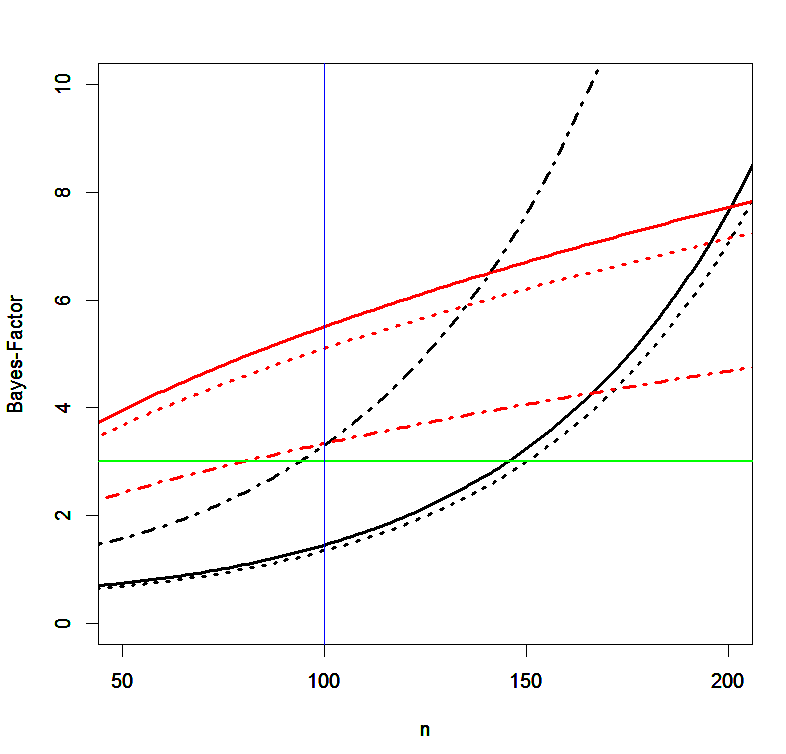
Dienes provided an online app to compute Bayes-Factors for these prior distributions. I used the posted r-code by John Christie to create the following figure. It shows Bayes-Factors for three a priori uniform distributions. Solid lines show Bayes-Factors for effect sizes in the range from 0 to 1. Dotted lines show effect sizes in the range from 0 to .5. The dot-line pattern shows Bayes-Factors for effect sizes in the range from .1 to .3. The most noteworthy observation is that prior distributions that are not centered over zero can actually provide evidence for a small effect with Bem’s (2011) sample sizes. The second observation is that these priors can also favor the null-hypothesis when the true effect size is zero (red lines). Bayes-Factors become more conclusive for more precisely formulate alternative hypotheses. The strongest evidence is obtained by contrasting the null-hypothesis with a narrow interval of possible effect sizes in the .1 to .3 range. The reason is that in this comparison weak effects below .1 clearly favor the null-hypothesis. For an expected effect size of d = .2, a range of values from 0 to .5 seems reasonable and can produce Bayes-Factors that exceed a value of 3 in studies with 100 to 200 participants. Thus, this is a reasonable prior for Bem’s studies.

WagF3

It is also possible to formulate alternative hypotheses with normal distributions around an a priori effect size. Dienes recommends setting the mean to 0 and to set the standard deviation of the expected effect size. The problem with this approach is again that the alternative hypothesis is centered over 0 (in a two-tailed test).   Moreover, the true effect size is not known. Like the scaling factor in the Cauchy distribution, using a higher value leads to a wider spread of alternative effect sizes and makes it harder to show evidence for small effects and easier to find evidence in favor of H0.   However, the r-code also allows specifying non-null means for the alternative hypothesis.   The next figure shows Bayes-Factors for three normally distributed alternative hypotheses. The solid lines show Bayes-Factors with mean = 0 and SD = .2. The dotted line shows Bayes-Factors for d = .2 (a small effect and the effect predicted by Bem) and a relatively wide standard deviation of .5. This means 95% of effect sizes are in the range from -.8 to 1.2. The broken (dot/dash) line shows Bayes-Factors with a mean of d = .2 and a narrower SD of d = .2. The 95% CI still covers a rather wide range of effect sizes from -.2 to .6, but due to the normal distribution effect sizes close to the expected effect size of d = .2 are weighted more heavily.

WagF4

The first observation is that centering the normal distribution over 0 leads to the same problem as the Cauchy-distribution. When the effect size is really 0, Bayes-Factors provide clear support for the null-hypothesis. However, when the effect size is small, d = .2, Bayes-Factors fail to provide support for the presence for samples with fewer than 150 participants (this is a ones-sample design, the equivalent sample size for between-subject designs is N = 600). The dotted line shows that simply moving the mean from d = 0 to d = .2 has relatively little effect on Bayes-Factors. Due to the wide range of effect sizes, a small effect is not sufficient to produce Bayes-Factors greater than 3 in small samples. The broken line shows more promising results. With d = .2 and SD = .2, Bayes-Factors in small samples with less than 100 participants are inconclusive. For sample sizes of more than 100 participants, both lines are above the criterion value of 3. This means, a Bayes-Factor of 3 or more can support the null-hypothesis when it is true and it can show that a small effect is present when an effect is present.

Another way to specify the alternative hypothesis is to use a one-tailed alternative hypothesis (a half-normal).   The mode (the center of the normal-distribution) of the distribution is 0. The solid line shows a standard deviation of .8. The dotted line shows results with standard deviation = .5 and the broken line shows results for a standard deviation of d = .2. The solid line favors the null-hypothesis and it requires sample sizes of more than 130 participants before an effect size of d = .2 produces a Bayes-Factor of 3 or more. In contrast, the broken line discriminates against the null-hypothesis and practically never supports the null-hypothesis when it is true. The dotted line with a standard deviation of .5 works best. It always shows support for the null-hypothesis when it is true and it can produce Bayes-Factors greater than 3 with a bit more than 100 participants.

WagF5

In conclusion, the simulations show that Bayes-Factors depend on the specification of the prior distribution and sample size. This has two implications. Unreasonable priors will lower the sensitivity/power of Bayes-Factors to support either the null-hypothesis or the alternative hypothesis when these hypotheses are true. Unreasonable priors will also bias the results in favor of one of the two hypotheses. As a result, researchers need to justify the choice of their priors and they need to be careful when they interpret results. It is particularly difficult to interpret Bayes-Factors when the alternative hypothesis is diffuse and the null-hypothesis is supported. In this case, the evidence merely shows that the null-hypothesis fits the data better than the alternative, but the alternative is a composite of many effect sizes and some of these effect sizes may fit the data better than the null-hypothesis.

Comparison of Different Prior Distributions with Bem’s (2011) ESP Experiments

To examine the influence of prior distributions on Bayes-Factors, I computed Bayes-Factors using several prior distributions. I used a d~Cauchy(1) distribution because this distribution was used by Wagenmakers et al. (2011). I used three uniform prior distributions with ranges of effect sizes from 0 to 1, 0 to .5, and .1 to .3. Based on Dienes recommendation, I also used a normal distribution centered on zero with the expected effect size as the standard deviation. I used both two-tailed and one-tailed (half-normal) distributions. Based on a twitter-recommendation by Alexander Etz, I also centered the normal distribution on the effect size, d = .2, with a standard deviation of d = .2.

Wag1 Table

The d~Cauchy(1) prior used by Wagenmakers et al. (2011) gives the weakest support for an effect. The table also includes the product of Bayes-Factors. The results confirm that the product is not a meaningful statistic that can be used to conduct a meta-analysis with Bayes-Factors. The last column shows Bayes-Factors based on a traditional fixed-effect meta-analysis of effect sizes in all 10 studies. Even the d~Cauchy(1) prior now shows strong support for the presence of an effect even though it often favored the null-hypotheses for individual studies. This finding shows that inferences about small effects in small samples cannot be trusted as evidence that the null-hypothesis is correct.

Table 1 also shows that all other prior distributions tend to favor the presence of an effect even in individual studies. Thus, these priors show consistent results for individual studies and for a meta-analysis of all studies. The strength of evidence for an effect is predictable from the precision of the alternative hypothesis. The uniform distribution with a wide range of effect sizes from 0 to 1, gives the weakest support, but it still supports the presence of an effect. This further emphasizes how unrealistic the Cauchy-distribution with a scaling factor of 1 is for most studies in psychology. For most studies in psychology effect sizes greater than 1 are rare. Moreover, effect sizes greater than one do not need fancy statistics. A simple visual inspection of a scatter plot is sufficient to reject the null-hypothesis. The strongest support for an effect is obtained for the uniform distribution with a range of effect sizes from .1 to .3. The advantage of this range is that the lower bound is not 0. Thus, effect sizes below the lower bound provide evidence for H0 and effect sizes above the lower bound provide evidence for an effect. The lower bound can be set by a meaningful consideration of what effect sizes might be theoretically or practically so small that they would be rather uninteresting even if they are real. Personally, I find uniform distributions appealing because they best express uncertainty about an effect size. Most theories in psychology do not make predictions about effect sizes. Thus, it seems impossible to say that an effect is expected to be small (d = .2) or moderate (d = .5). It seems easier to say that an effect is expected to be small (d = .1 to .3) or moderate (.3 to .6) or large (.6 to 1). Cohen used fixed values only because power analysis requires a single value. As Bayesian statistics allows the specification of ranges, it makes sense to specify a range of values with the need to make predictions which values in this range are more likely. However, results for the normal distribution provide similar results. Again, the strength of evidence of an effect increases with the precision of the predicted effect. The weakest support for an effect is obtained with a normal distribution centered over 0 and a two-tailed test. This specification is similar to a Cauchy distribution but it uses the normal distribution. However, by setting the standard deviation to the expected effect sizes, Bayes-Factors show evidence for an effect. The evidence for an effect becomes stronger by centering the distribution over the expected effect size or by using a half-normal (one-tailed) test that makes predictions about the direction of the effect.

To summarize, the main point is that Bayes-Factors depend on the choice of the alternative distribution. Bayesian statisticians are of course well aware of this fact. However, in practical applications of Bayesian statistics, the importance of the prior distribution is often ignored, especially when Bayes-Factors favor the null-hypothesis. Although this finding only means that the data support the null-hypothesis more than the alternative hypothesis, the alternative hypothesis is often described in vague terms as a hypothesis that predicted an effect. However, the alternative hypothesis does not just predict that there is an effect. It makes predictions about the strength of effects and it is always possible to specify an alternative that predicts an effect that is still consistent with the data by choosing a small effect size. Thus, Bayesian statistics can only produce meaningful results if researchers specify a meaningful alternative hypothesis. It is therefore surprising how little attention Bayesian statisticians have devoted to the issue of specifying the prior distribution. The most useful advice comes from Dienes recommendation to specify the prior distribution as a normal distribution centered over 0 and to set the standard deviation to the expected effect size. If researchers are uncertain about the effect size, they could try different values for small (d = .2), moderate (d = .5), or large (d = .8) effect sizes. Researchers should be aware that the current default setting of .707 in Rouder’s online app implies an expectation of a strong effect and that this setting will make it harder to show evidence for small effects and inflates the risk of obtaining false support for the null-hypothesis.

Why Psychologists Should not Change the Way They Analyze Their Data

Wagenmakers et al. (2011) did not simply use Bayes-Factors to re-examine Bem’s claims about ESP. Like several other authors, they considered Bem’s (2011) article an example of major flaws in psychological science. Thus, they titled their article with the rather strong admonition that “Psychologists Must Change The Way They Analyze Their Data.”   They blame the use of p-values and significance tests as the root cause of all problems in psychological science. “We conclude that Bem’s p values do not indicate evidence in favor of precognition; instead, they indicate that experimental psychologists need to change the way they conduct their experiments and analyze their data” (p. 426). The crusade against p-values starts with the claim that it is easy to obtain data that reject the null-hypothesis even when the null-hypothesis is true. “These experiments highlight the relative ease with which an inventive researcher can produce significant results even when the null hypothesis is true” (p. 427). However, this statement is incorrect. The probability of getting significant results is clearly specified by the type-I error rate. When the null-hypothesis is true, a significant result will emerge only 5% of the time; that is in 1 out of 20 studies. The probability of making a type-I error repeatedly decrease exponentially. For two studies, the probability to obtain two type-I errors is only p = .0025 or 1 out of 400 (20 * 20 studies).   If some non-significant results are obtained, the binomial probability gives the probability that the frequency of significant results that could have been obtained if the null-hypothesis were true. Bem obtained 9 out of 10 significant results. With a probability of p = .05, the binomial probability is 18e-10. Thus, there is strong evidence that Bem’s results are not type-I errors. He did not just go in his lab and run 10 studies and obtained 9 significant results by chance alone. P-values correctly quantify how unlikely this event is in a single study and how this probability decrease as the number of studies increases. The table also shows that all Bayes-Factors confirm this conclusion when the results of all studies are combined in a meta-analysis.   It is hard to see how p-values can be misleading when they lead to the same conclusion as Bayes-Factors. The combined evidence presented by Bem cannot be explained by random sampling error. The data are inconsistent with the null-hypothesis. The only misleading statistic is provided by a Bayes-Factor with an unreasonable prior distribution of effect sizes in small samples. All other statistics agree that the data show an effect.

Wagenmakers et al. (2011) next argument is that p-values only consider the conditional probability when the null-hypothesis is true, but that it is also important to consider the conditional probability if the alternative hypothesis is true. They fail to mention, however, that this alternative hypothesis is equivalent to the concept of statistical power. A p-values of less than .05 means that a significant result would be obtained only 5% of the time when the null-hypothesis is true. The probability of a significant result when an effect is present depends on the size of the effect and sampling error and can be computed using standard tools for power analysis. Importantly, Bem (2011) actually carried out an a priori power analysis and planned his studies to have 80% power. In a one-sample t-test, standard error is defined as 1/sqrt(N). Thus, with 100 participants, the standard error is .1. With an effect size of d = .2, the signal-to-noise ratio is .2/.1 = 2. Using a one-tailed significance test, the criterion value for significance is 1.66. The implied power is 63%. Bem used an effect size of d = .25 to suggest that he has 80% power. Even with a conservative estimate of 50% power, the likelihood ratio of obtaining a significant is .50/.05 = 10. This likelihood ratio can be interpreted like Bayes-Factors. Thus, in a study with 50% power, it is 10 times more likely to obtain a significant result when an effect is present than when the null-hypothesis is true. Thus, even in studies with modest power, favors the alternative hypothesis much more than the null-hypothesis. To argue that p-values provide weak evidence for an effect implies that a study had very low power to show an effect. For example, if a study has only 10% power, the likelihood ratio is only 2 in favor of an effect being present. Importantly, low power cannot explain Bem’s results because low power would imply that most studies produced non-significant results. However, he obtained 9 significant results in 10 studies. This success rate is itself an estimate of power and would suggest that Bem had 90% power in his studies. With 90% power, the likelihood ratio is .90/.05 = 18. The Bayesian argument against p-values is only valid for the interpretation of p-values in a single study in the absence of any information about power. Not surprisingly, Bayesians often focus on Fisher’s use of p-values. However, Neyman-Pearson emphasized the need to also consider type-II error rates and Cohen has emphasized the need to conduct power analysis to ensure that small effects can be detected. In recent years, there has been an encouraging trend to increase power of studies. One important consequence of high powered studies is that significant results increase the evidential value of significant results because a significant result is much more likely to emerge when an effect is present than when it is not present. However, it is important to note that the most likely outcome in underpowered studies is a non-significant result. Thus, it is unlikely that a set of studies can produce false evidence for an effect because a meta-analysis would reveal that most studies fail to show an effect. The main reason for the replication crisis in psychology is the practice not to report non-significant results. This is not a problem of p-values, but a problem of selective reporting. However, Bayes-Factors are not immune to reporting biases. As Table 1 shows, it would have been possible to provide strong evidence for ESP using Bayes-Factors as well.

To demonstrate the virtues of Bayesian statistics, Wagenmakers et al. (2011) then presented their Bayesian analyses of Bem’s data. What is important here, is how the authors explain the choice of their priors and how the authors interpret their results in the context of the choice of their priors.   The authors state that they “computed a default Bayesian t test” (p. 430). The important word is default. This word makes it possible to present a Bayesian analysis without a justification of the prior distribution. The prior distribution is the default distribution, a one-size-fits-all prior that does not need any further elaboration. The authors do note that “more specific assumptions about the effect size of psi would result in a different test.” (p. 430). They do not mention that these different tests would also lead to different conclusions because the conclusion is always relative to the specified alternative hypothesis. Even less convincing is their claim that “we decided to first apply the default test because we did not feel qualified to make these more specific assumptions, especially not in an area as contentious as psi” (p. 430). It is true that the authors are not experts on PSI, but that is hardly necessary when Bem (2011) presented a meta-analysis and  made an a prior prediction about effect size. Moreover, they could have at least used a half-Cauchy given that Bem used one-tailed tests.

The results of the default t-test are then used to suggest that “a default Bayesian test confirms the intuition that, for large sample sizes, one-sided p values higher than .01 are not compelling” (p. 430). This statement ignores their own critique of p-values that the compelingness of p-values depends on the power of a study. A p-value of .01 in a study with 10% power is not compelling because it is very unlikely outcome no matter whether an effect is present or not. However, in a study with 50% power, a p-value of .01 is very compelling because the likelihood ratio is 50. That is, it is 50 times more likely to get a significant result at p = .01 in a study with 50% power when an effect is present than when an effect is not present.

The authors then emphasize that they “did not select priors to obtain a desired result” (p. 430). This statement can be confusing to non-Bayesian readers. What this statement means is that Bayes-Factors do not entail statements about the probability that ESP exists or does not exist. However, Bayes-Factors do require specification of a prior distribution. Thus, the authors did select a prior distribution, namely the default distribution, and Table 1 shows that their choice of the prior distribution influenced the results.

The authors do directly address the choice of the prior distribution and state “we also examined other options, however, and found that our conclusions were robust. For a wide range of different non-default prior distributions on effect sizes, the evidence for precognition is either non-existent or negligible” (p. 430). These results are reported in a supplementary document. In these materials., the authors show how the scaling factor clearly influences results and that small scaling factors suggest an effect is present whereas larger scaling factors favor the null-hypothesis. However, Bayes-Factors in favor of an effect are not very strong. The reason is that the prior distribution is centered over 0 and a two-tailed test is being used. This makes it very difficult to distinguish the null-hypothesis from the alternative hypothesis. As shown in Table 1, priors that contrast the null-hypothesis with an effect provide much stronger evidence for the presence of an effect. In their conclusion, the authors state “In sum, we conclude that our results are robust to different specifiications of the scale parameter for the effect size prior under H1 “ This statement is more correct than the statement in the article, where they claim that they considered a wide range of non-default prior distributions. They did not consider a wide range of different distributions. They considered a wide range of scaling parameters for a single distribution; a Cauchy-distribution centered over 0.   If they had considered a wide range of prior distributions, like I did in Table 1, they would have found that Bayes-Factors for some prior distributions suggest that an effect is present.

The authors then deal with the concern that Bayes-Factors depend on sample size and that larger samples might lead to different conclusions, especially when smaller samples favor the null-hypothesis. “At this point, one may wonder whether it is feasible to use the Bayesian t test and eventually obtain enough evidence against the null hypothesis to overcome the prior skepticism outlined in the previous section.” The authors claimed that they are biased against the presence of an effect by a factor of 10e-24. Thus, it would require a Bayes-Factor greater than 10e24 to sway them that ESP exists. They then point out that the default Bayesian t-test, a Cauchi(0,1) prior distribution, would produce this Bayes-Factor in a sample of 2,000 participants. They then propose that a sample size of N = 2,000 is excessive. This is not a principled robustness analysis. A much easier way to examine what would happen in a larger sample, is to conduct a meta-analysis of the 10 studies, which already included 1,196 participants. As shown in Table 1, the meta-analysis would have revealed that even the default t-test favors the presence of an effect over the null-hypothesis by a factor of 6.55e10.   This is still not sufficient to overcome prejudice against an effect of a magnitude of 10e-24, but it would have made readers wonder about the claim that Bayes-Factors are superior than p-values. There is also no need to use Bayesian statistics to be more skeptical. Skeptical researchers can also adjust the criterion value of a p-value if they want to lower the risk of a type-I error. Editors could have asked Bem to demonstrate ESP with p < .001 rather than .05 in each study, but they considered 9 out of 10 significant results at p < .05 (one-tailed) sufficient. As Bayesians provide no clear criterion values when Bayes-Factors are sufficient, Bayesian statistics does not help editors in the decision process how strong evidence has to be.

Does This Mean ESP Exists?

As I have demonstrated, even Bayes-Factors using the most unfavorable prior distribution favors the presence of an effect in a meta-analysis of Bem’s 10 studies. Thus, Bayes-Factors and p-values strongly suggest that Bem’s data are not the result of random sampling error. It is simply too improbable that 9 out of 10 studies produce significant results when the null-hypothesis is true. However, this does not mean that Bem’s data provide evidence for a real effect because there are two explanations for systematic deviations from a random pattern (Schimmack, 2012). One explanation is that a true effect is present and that a study had good statistical power to produce a signal-to-noise ratio that produces a significant outcome. The other explanation is that no true effect is present, but that the reported results were obtained with the help of questionable research practices that inflate the type-I error rate. In a multiple study article, publication bias cannot explain the result because all studies were carried out by the same researcher. Publication bias can only occur when a researcher conducts a single study and reports a significant result that was obtained by chance alone. However, if a researcher conducts multiple studies, type-I errors will not occur again and again and questionable research practices (or fraud) are the only explanation for significant results when the null-hypothesis is actually true.

There have been numerous analyses of Bem’s (2011) data that show signs of questionable research practices (Francis, 2012; Schimmack, 2012; Schimmack, 2015). Moreover, other researchers have failed to replicate Bem’s results. Thus, there is no reason to believe in ESP based on Bem’s data even though Bayes-Factors and p-values strongly reject the hypothesis that sample means are just random deviations from 0. However, the problem is not that the data were analyzed with the wrong statistical method. The reason is that the data are not credible. It would be problematic to replace the standard t-test with the default Bayesian t-test because the default Bayesian t-test gives the right answer with questionable data. The reason is that it would give the wrong answer with credible data, namely it would suggest that no effect is present when a researcher conducts 10 studies with 50% power and honestly reports 5 non-significant results. Rather than correctly inferring from this pattern of results that an effect is present, the default-Bayesian t-test, when applied to each study individually, would suggest that the evidence is inconclusive.

Conclusion

There are many ways to analyze data. There are also many ways to conduct Bayesian analysis. The stronger the empirical evidence is, the less important the statistical approach will be. When different statistical approaches produce different results, it is important to carefully examine the different assumptions of statistical tests that lead to the different conclusions based on the same data. There is no superior statistical method. Never trust a statistician who tells you that you are using the wrong statistical method. Always ask for an explanation why one statistical method produces one result and why another statistical method produces a different result. If one method seems to make more reasonable assumptions than another (data are not normally distributed, unequal variances, unreasonable assumptions about effect size), use the more reasonable statistical method. I have repeatedly asked Dr. Wagenmakers to justify his choice of the Cauchi(0,1) prior, but he has not provide any theoretical or statistical arguments for this extremely wide range of effect sizes.

So, I do not think that psychologists need to change the way they analyze their data. In studies with reasonable power (50% or more), significant results are much more likely to occur when an effect is present than when an effect is not present, and likelihood ratios will show similar results as Bayes-Factors with reasonable priors. Moreover, the probability of a type-I errors in a single study is less important for researchers and science than long-term rate of type-II errors. Researchers need to conduct many studies to build up a CV, get jobs, grants, and take care of their graduate students. Low powered studies will lead to many non-significant results that provide inconclusive results. Thus, they need to conduct powerful studies to be successful. In the past, researchers often used questionable research practices to increase power without declaring the increased risk of a type-I error. However, in part due to Bem’s (2011) infamous article, questionable research practices are becoming less acceptable and direct replication attempts more quickly reveal questionable evidence. In this new culture of open science, only researchers who carefully plan studies will be able to provide consistent empirical support for a theory because the theory actually makes correct predictions. Once researchers report all of the relevant data, it is less important how these data are analyzed. In this new world of psychological science, it will be problematic to ignore power and to use the default Bayesian t-test because it will typically show no effect. Unless researches are planning to build a career on confirming the absence of effects, they should conduct studies with high-power and control type-I error rates by replicating and extending their own work.

Bayesian Statistics in Small Samples: Replacing Prejudice against the Null-Hypothesis with Prejudice in Favor of the Null-Hypothesis

Matzke, Nieuwenhuis, van Rijn, Slagter, van der Molen, and Wagenmakers (2015) published the results of a preregistered adversarial collaboration. This article has been considered a model of conflict resolution among scientists.

The study examined the effect of eye-movements on memory. Drs. Nieuwenhuis and Slagter assume that horizontal eye-movements improve memory. Drs. Matzke, van Rijn, and Wagenmakers did not believe that horizontal-eye movements improve memory. That is, they assumed the null-hypothesis to be true. Van der Molen acted as a referee to resolve conflict about procedural questions (e.g., should some participants be excluded from analysis?).

The study was a between-subject design with three conditions: horizontal eye movements, vertical eye movements, and no eye movement.

The researchers collected data from 81 participants and agreed to exclude 2 participants, leaving 79 participants for analysis. As a result there were 27 or 26 participants per condition.

The hypothesis that horizontal eye-movements improve performance can be tested in several ways.

An overall F-test can compare the means of the three groups against the hypothesis that they are all equal. This test has low power because nobody predicted differences between vertical eye-movements and no eye-movements.

A second alternative is to compare the horizontal condition against the combined alternative groups. This can be done with a simple t-test. Given the directed hypothesis, a one-tailed test can be used.

Power analysis with the free software program GPower shows that this design has 21% power to reject the null-hypothesis with a small effect size (d = .2). Power for a moderate effect size (d = .5) is 68% and power for a large effect size (d = .8) is 95%.

Thus, the decisive study that was designed to solve the dispute only has adequate power (95%) to test Drs. Matzke et al.’s hypothesis d = 0 against the alternative hypothesis that d = .8. For all effect sizes between 0 and .8, the study was biased in favor of the null-hypothesis.

What does an effect size of d = .8 mean? It means that memory performance is boosted by .8 standard deviations. For example, if students take a multiple-choice exam with an average of 66% correct answers and a standard deviation of 15%, they could boost their performance by 12% points (15 * 0.8 = 12) from an average of 66% (C) to 78% (B+) by moving their eyes horizontally while thinking about a question.

The article makes no mention of power-analysis and the implicit assumption that the effect size has to be large to avoid biasing the experiment in favor of the critiques.

Instead the authors used Bayesian statistics; a type of statistics that most empirical psychologists understand even less than standard statistics. Bayesian statistics somehow magically appears to be able to draw inferences from small samples. The problem is that Bayesian statistics requires researchers to specify a clear alternative to the null-hypothesis. If the alternative is d = .8, small samples can be sufficient to decide whether an observed effect size is more consistent with d = 0 or d = .8. However, with more realistic assumptions about effect sizes, small samples are unable to reveal whether an observed effect size is more consistent with the null-hypothesis or a small to moderate effect.

Actual Results

So what where the actual results?

Condition                                          Mean     SD         

Horizontal Eye-Movements          10.88     4.32

Vertical Eye-Movements               12.96     5.89

No Eye Movements                       15.29     6.38      

The results provide no evidence for a benefit of horizontal eye movements. In a comparison of the two a priori theories (d = 0 vs. d > 0), the Bayes-Factor strongly favored the null-hypothesis. However, this does not mean that Bayesian statistics has magical powers. The reason was that the empirical data actually showed a strong effect in the opposite direction, in that participants in the no-eye-movement condition had better performance than in the horizontal-eye-movement condition (d = -.81).   A Bayes Factor for a two-tailed hypothesis or the reverse hypothesis would not have favored the null-hypothesis.

Conclusion

In conclusion, a small study surprisingly showed a mean difference in the opposite prediction than previous studies had shown. This finding is noteworthy and shows that the effects of eye-movements on memory retrieval are poorly understood. As such, the results of this study are simply one more example of the replicability crisis in psychology.

However, it is unfortunate that this study is published as a model of conflict resolution, especially as the empirical results failed to resolve the conflict. A key aspect of a decisive study is to plan a study with adequate power to detect an effect.   As such, it is essential that proponents of a theory clearly specify the effect size of their predicted effect and that the decisive experiment matches type-I and type-II error. With the common 5% Type-I error this means that a decisive experiment must have 95% power (1 – type II error). Bayesian statistics does not provide a magical solution to the problem of too much sampling error in small samples.

Bayesian statisticians may ignore power analysis because it was developed in the context of null-hypothesis testing. However, Bayesian inferences are also influenced by sample size and studies with small samples will often produce inconclusive results. Thus, it is more important that psychologists change the way they collect data than to change the way they analyze their data. It is time to allocate more resources to fewer studies with less sampling error than to waste resources on many studies with large sampling error; or as Cohen said: Less is more.