In 2011 I wrote a manuscript in response to Bem’s (2011) unbelievable and flawed evidence for extroverts’ supernatural abilities. It took nearly two years for the manuscript to get published in Psychological Methods. While I was proud to have published in this prestigious journal without formal training in statistics and a grasp of Greek notation, I now realize that Psychological Methods was not the best outlet for the article, which may explain why even some established replication revolutionaries do not know it (comment: I read your blog, but I didn’t know about this article). So, I decided to publish an abridged (it is still long), lightly edited (I have learned a few things since 2011), and commented (comments are in […]) version here.
I also learned a few things about titles. So the revised version, has a new title.
Finally, I can now disregard the request from the editor, Scott Maxwell, on behave of reviewer Daryl Bem, to change the name of my statistical index from magic index to incredibilty index. (the advantage of publishing without the credentials and censorship of peer-review).
For readers not familiar with experimental social psychology, it is also important to understand what a multiple study article is. Most science are happy with one empirical study per article. However, social psychologists didn’t trust the results of a single study with p < .05. Therefore, they wanted to see internal conceptual replications of phenomena. Magically, Bem was able to provide evidence for supernatural abilities in not just 1 or 2 or 3 studies, but 8 conceptual replication studies with 9 successful tests. The chance of a false positive result in 9 statistical tests is smaller than the chance of finding evidence for the Higgs-Bosson particle, which was a big discovery in physics. So, readers in 2011 had a difficult choice to make: either supernatural phenomena are real or multiple study articles are unreal. My article shows that the latter is likely to be true, as did an article by Greg Francis.
Aside from Alcock’s demonstration of a nearly perfect negative correlation between effect sizes and sample sizes and my demonstration of insufficient variance in Bem’s p-values, Francis’s article and my article remain the only article that question the validity of Bem’s origina findings. Other articles have shown that the results cannot be replicated, but I showed that the original results were already too good to be true. This blog post explains, how I did it.
Why most multiple-study articles are false: An Introduction to the Magic Index
(the article formerly known as “The Ironic Effect of Significant Results on the Credibility of Multiple-Study Articles”)
ABSTRACT
Cohen (1962) pointed out the importance of statistical power for psychology as a science, but statistical power of studies has not increased, while the number of studies in a single article has increased. It has been overlooked that multiple studies with modest power have a high probability of producing nonsignificant results because power decreases as a function of the number of statistical tests that are being conducted (Maxwell, 2004). The discrepancy between the expected number of significant results and the actual number of significant results in multiple-study articles undermines the credibility of the reported
results, and it is likely that questionable research practices have contributed to the reporting of too many significant results (Sterling, 1959). The problem of low power in multiple-study articles is illustrated using Bem’s (2011) article on extrasensory perception and Gailliot et al.’s (2007) article on glucose and self-regulation. I conclude with several recommendations that can increase the credibility of scientific evidence in psychological journals. One major recommendation is to pay more attention to the power of studies to produce positive results without the help of questionable research practices and to request that authors justify sample sizes with a priori predictions of effect sizes. It is also important to publish replication studies with nonsignificant results if these studies have high power to replicate a published finding.
Keywords: power, publication bias, significance, credibility, sample size
INTRODUCTION
Less is more, except of course for sample size. (Cohen, 1990, p. 1304)
In 2011, the prestigious Journal of Personality and Social Psychology published an article that provided empirical support for extrasensory perception (ESP; Bem, 2011). The publication of this controversial article created vigorous debates in psychology
departments, the media, and science blogs. In response to this debate, the acting editor and the editor-in-chief felt compelled to write an editorial accompanying the article. The editors defended their decision to publish the article by noting that Bem’s (2011) studies were performed according to standard scientific practices in the field of experimental psychology and that it would seem inappropriate to apply a different standard to studies of ESP (Judd & Gawronski, 2011).
Others took a less sanguine view. They saw the publication of Bem’s (2011) article as a sign that the scientific standards guiding publication decisions are flawed and that Bem’s article served as a glaring example of these flaws (Wagenmakers, Wetzels, Borsboom,
& van der Maas, 2011). In a nutshell, Wagenmakers et al. (2011) argued that the standard statistical model in psychology is biased against the null hypothesis; that is, only findings that are statistically significant are submitted and accepted for publication.
This bias leads to the publication of too many positive (i.e., statistically significant) results. The observation that scientific journals, not only those in psychology,
publish too many statistically significant results is by no means novel. In a seminal article, Sterling (1959) noted that selective reporting of statistically significant results can produce literatures that “consist in substantial part of false conclusions” (p.
30).
Three decades later, Sterling, Rosenbaum, and Weinkam (1995) observed that the “practice leading to publication bias have [sic] not changed over a period of 30 years” (p. 108). Recent articles indicate that publication bias remains a problem in psychological
journals (Fiedler, 2011; John, Loewenstein, & Prelec, 2012; Kerr, 1998; Simmons, Nelson, & Simonsohn, 2011; Strube, 2006; Vul, Harris, Winkielman, & Pashler, 2009; Yarkoni, 2010).
Other sciences have the same problem (Yong, 2012). For example, medical journals have seen an increase in the percentage of retracted articles (Steen, 2011a, 2011b), and there is the concern that a vast number of published findings may be false (Ioannidis,
2005).
However, a recent comparison of different scientific disciplines suggested that the bias is stronger in psychology than in some of the older and harder scientific disciplines at the top of a hierarchy of sciences (Fanelli, 2010).
It is important that psychologists use the current crisis as an opportunity to fix problems in the way research is being conducted and reported. The proliferation of eye-catching claims based on biased or fake data can have severe negative consequences for a
science. A New Yorker article warned the public that “all sorts of well-established, multiply confirmed findings have started to look increasingly uncertain. It’s as if our facts were losing their truth: claims that have been enshrined in textbooks are suddenly unprovable” (Lehrer, 2010, p. 1).
If students who read psychology textbooks and the general public lose trust in the credibility of psychological science, psychology loses its relevance because
objective empirical data are the only feature that distinguishes psychological science from other approaches to the understanding of human nature and behavior. It is therefore hard to exaggerate the seriousness of doubts about the credibility of research findings published in psychological journals.
In an influential article, Kerr (1998) discussed one source of bias, namely, hypothesizing after the results are known (HARKing). The practice of HARKing may be attributed to the
high costs of conducting a study that produces a nonsignificant result that cannot be published. To avoid this negative outcome, researchers can design more complex studies that test multiple hypotheses. Chances increase that at least one of the hypotheses
will be supported, if only because Type I error increases (Maxwell, 2004). As noted by Wagenmakers et al. (2011), generations of graduate students were explicitly advised that this questionable research practice is how they should write scientific manuscripts
(Bem, 2000).
It is possible that Kerr’s (1998) article undermined the credibility of single-study articles and added to the appeal of multiple-study articles (Diener, 1998; Ledgerwood & Sherman, 2012). After all, it is difficult to generate predictions for significant effects
that are inconsistent across studies. Another advantage is that the requirement of multiple significant results essentially lowers the chances of a Type I error, that is, the probability of falsely rejecting the null hypothesis. For a set of five independent studies,
the requirement to demonstrate five significant replications essentially shifts the probability of a Type I error from p < .05 for a single study to p < .0000003 (i.e., .05^5) for a set of five studies.
This is approximately the same stringent criterion that is being used in particle physics to claim a true discovery (Castelvecchi, 2011). It has been overlooked, however, that researchers have to pay a price to meet more stringent criteria of credibility. To demonstrate significance at a more stringent criterion of significance, it is
necessary to increase sample sizes to reduce the probability of making a Type II error (failing to reject the null hypothesis). This probability is called beta. The inverse probability (1 – beta) is called power. Thus, to maintain high statistical power to demonstrate an effect with a more stringent alpha level requires an
increase in sample sizes, just as physicists had to build a bigger collider to have a chance to find evidence for smaller particles like the Higgs boson particle.
Yet there is no evidence that psychologists are using bigger samples to meet more stringent demands of replicability (Cohen, 1992; Maxwell, 2004; Rossi, 1990; Sedlmeier & Gigerenzer, 1989). This raises the question of how researchers are able to replicate findings in multiple-study articles despite modest power to demonstrate significant effects even within a single study. Researchers can use questionable research
practices (e.g., snooping, not reporting failed studies, dropping dependent variables, etc.; Simmons et al., 2011; Strube, 2006) to dramatically increase the chances of obtaining a false-positive result. Moreover, a survey of researchers indicated that these
practices are common (John et al., 2012), and the prevalence of these practices has raised concerns about the credibility of psychology as a science (Yong, 2012).
An implicit assumption in the field appears to be that the solution to these problems is to further increase the number of positive replication studies that need to be presented to ensure scientific credibility (Ledgerwood & Sherman, 2012). However, the assumption that many replications with significant results provide strong evidence for a hypothesis is an illusion that is akin to the Texas sharpshooter fallacy (Milloy, 1995). Imagine a Texan farmer named Joe. One day he invites you to his farm and shows you a target with nine shots in the bull’s-eye and one shot just outside the bull’s-eye. You are impressed by his shooting abilities until you find out that he cannot repeat this performance when you challenge him to do it again.
[So far, well-known Texan sharpshooters in experimental social psychology have carefully avoided demonstrating their sharp shooting abilities in open replication studies to avoid the embarrassment of not being able to do it again].
Over some beers, Joe tells you that he first fired 10 shots at the barn and then drew the targets after the shots were fired. One problem in science is that reading a research
article is a bit like visiting Joe’s farm. Readers only see the final results, without knowing how the final results were created. Is Joe a sharpshooter who drew a target and then fired 10 shots at the target? Or was the target drawn after the fact? The reason why multiple-study articles are akin to a Texan sharpshooter is that psychological studies have modest power (Cohen, 1962; Rossi, 1990; Sedlmeier & Gigerenzer, 1989). Assuming
60% power for a single study, the probability of obtaining 10 significant results in 10 studies is less than 1% (.6^10 = 0.6%).
I call the probability to obtain only significant results in a set of studies total power. Total power parallels Maxwell’s (2004) concept of all-pair power for multiple comparisons in analysis-of variance designs. Figure 1 illustrates how total power decreases with the number of studies that are being conducted. Eventually, it becomes extremely unlikely that a set of studies produces only significant results. This is especially true if a single study has modest power. When total power is low, it is incredible that a set
of studies yielded only significant results. To avoid the problem of incredible results, researchers would have to increase the power of studies in multiple-study articles.
Table 1 shows how the power of individual studies has to be adjusted to maintain 80% total power for a set of studies. For example, to have 80% total power for five replications, the power of each study has to increase to 96%.
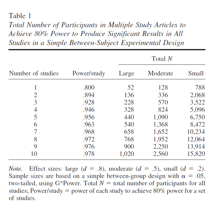
Table 1 also shows the sample sizes required to achieve 80% total power, assuming a simple between-group design, an alpha level of .05 (two-tailed), and Cohen’s
(1992) guidelines for a small (d = .2), moderate, (d = .5), and strong (d = .8) effect.
[To demonstrate a small effect 7 times would require more than 10,000 participants.]
In sum, my main proposition is that psychologists have falsely assumed that increasing the number of replications within an article increases credibility of psychological science. The problem of this practice is that a truly programmatic set of multiple studies
is very costly and few researchers are able to conduct multiple studies with adequate power to achieve significant results in all replication attempts. Thus, multiple-study articles have intensified the pressure to use questionable research methods to compensate for low total power and may have weakened rather than strengthened
the credibility of psychological science.
[I believe this is one reason why the replication crisis has hit experimental social psychology the hardest. Other psychologists could use HARKing to tell a false story about a single study, but experimental social psychologists had to manipulate the data to get significance all the time. Experimental cognitive psychologists also have multiple study articles, but they tend to use more powerful within-subject designs, which makes it more credible to get significant results multiple times. The multiple study BS design made it impossible to do so, which resulted in the publication of BS results.]
What Is the Allure of Multiple-Study Articles?
One apparent advantage of multiple-study articles is to provide stronger evidence against the null hypothesis (Ledgerwood & Sherman, 2012). However, the number of studies is irrelevant because the strength of the empirical evidence is a function of the
total sample size rather than the number of studies. The main reason why aggregation across studies reduces randomness as a possible explanation for observed mean differences (or correlations) is that p values decrease with increasing sample size. The
number of studies is mostly irrelevant. A study with 1,000 participants has as much power to reject the null hypothesis as a meta-analysis of 10 studies with 100 participants if it is reasonable to assume a common effect size for the 10 studies. If true effect sizes vary across studies, power decreases because a random-effects model may be more appropriate (Schmidt, 2010; but see Bonett, 2009). Moreover, the most logical approach to reduce concerns about Type I error is to use more stringent criteria for significance (Mudge, Baker, Edge, & Houlahan, 2012). For controversial or very important research findings, the significance level could be set to p < .001 or, as in particle physics, to p <
.0000005.
[Ironically, five years later we have a debate about p < .05 versus p < .005, without even thinking about p < .0000005 or any mention that even a pair of studies with p < .05 in each study effectively have an alpha less than p < .005, namely .0025 to be exact.]
It is therefore misleading to suggest that multiple-study articles are more credible than single-study articles. A brief report with a large sample (N = 1,000) provides more credible evidence than a multiple-study article with five small studies (N = 40, total
N = 200).
The main appeal of multiple-study articles seems to be that they can address other concerns (Ledgerwood & Sherman, 2012). For example, one advantage of multiple studies could be to test the results across samples from diverse populations (Henrich, Heine, & Norenzayan, 2010). However, many multiple-study articles are based on samples drawn from a narrowly defined population (typically, students at the local university). If researchers were concerned about generalizability across a wider range of individuals, multiple-study articles should examine different populations. However, it is not clear why it would be advantageous to conduct multiple independent studies with different populations. To compare populations, it would be preferable to use the same procedures and to analyze the data within a single statistical model with population as a potential moderating factor. Moreover, moderator tests often have low power. Thus, a single study with a large sample and moderator variables is more informative than articles that report separate analyses with small samples drawn from different populations.
Another attraction of multiple-study articles appears to be the ability to provide strong evidence for a hypothesis by means of slightly different procedures. However, even here, single studies can be as good as multiple-study articles. For example, replication across different dependent variables in different studies may mask the fact that studies included multiple dependent variables and researchers picked dependent variables that produced significant results (Simmons et al., 2011). In this case, it seems preferable to
demonstrate generalizability across dependent variables by including multiple dependent variables within a single study and reporting the results for all dependent variables.
One advantage of a multimethod assessment in a single study is that the power to
demonstrate an effect increases for two reasons. First, while some dependent variables may produce nonsignificant results in separate small studies due to low power (Maxwell, 2004), they may all show significant effects in a single study with the total sample size
of the smaller studies. Second, it is possible to increase power further by constraining coefficients for each dependent variable or by using a latent-variable measurement model to test whether the effect is significant across dependent variables rather than for each one independently.
Multiple-study articles are most common in experimental psychology to demonstrate the robustness of a phenomenon using slightly different experimental manipulations. For example, Bem (2011) used a variety of paradigms to examine ESP. Demonstrating
a phenomenon in several different ways can show that a finding is not limited to very specific experimental conditions. Analogously, if Joe can hit the bull’s-eye nine times from different angles, with different guns, and in different light conditions, Joe
truly must be a sharpshooter. However, the variation of experimental procedures also introduces more opportunities for biases (Ioannidis, 2005).
[This is my take down of social psychologists’ claim that multiple conceptual replications test theories, Stroebe & Strack, 2004]
The reason is that variation of experimental procedures allows researchers to discount null findings. Namely, it is possible to attribute nonsignificant results to problems with the experimental procedure rather than to the absence of an effect. In this way, empirical studies no longer test theoretical hypotheses because they can only produce two results: Either they support the theory (p < .05) or the manipulation did not work (p > .05). It is therefore worrisome that Bem noted that “like most social psychological experiments, the experiments reported here required extensive pilot testing” (Bem, 2011, p. 421). If Joe is a sharpshooter, who can hit the bull’s-eye from different angles and with different guns, why does he need extensive training before he can perform the critical shot?
The freedom of researchers to discount null findings leads to the paradox that conceptual replications across multiple studies give the impression that an effect is robust followed by warnings that experimental findings may not replicate because they depend “on subtle and unknown factors” (Bem, 2011, p. 422).
If experimental results were highly context dependent, it would be difficult to explain how studies reported in research articles nearly always produce the expected results. One possible explanation for this paradox is that sampling error in small samples creates the illusion that effect sizes vary systematically, although most of the variation is random. Researchers then pick studies that randomly produced inflated effect sizes and may further inflate them by using questionable research methods to achieve significance (Simmons et al., 2011).
[I was polite when I said “may”. This appears to be exactly what Bem did to get his supernatural effects.]
The final set of studies that worked is then published and gives a false sense of the effect size and replicability of the effect (you should see the other side of Joe’s barn). This may explain why research findings initially seem so impressive, but when other researchers try to build on these seemingly robust findings, it becomes increasingly uncertain whether a phenomenon exists at all (Ioannidis, 2005; Lehrer, 2010).
At this point, a lot of resources have been wasted without providing credible evidence for an effect.
[And then Stroebe and Strack in 2014 suggest that real replication studies that let the data determine the outcome are a waste of resources.]
To increase the credibility of reported findings, it would be better to use all of the resources for one powerful study. For example, the main dependent variable in Bem’s (2011) study of ESP was the percentage of correct predictions of future events.
Rather than testing this ability 10 times with N = 100 participants, it would have been possible to test the main effect of ESP in a single study with 10 variations of experimental procedures and use the experimental conditions as a moderating factor. By testing one
main effect of ESP in a single study with N = 1,000, power would be greater than 99.9% to demonstrate an effect with Bem’s a priori effect size.
At the same time, the power to demonstrate significant moderating effects would be much lower. Thus, the study would lead to the conclusion that ESP does exist but that it is unclear whether the effect size varies as a function of the actual experimental
paradigm. This question could then be examined in follow-up studies with more powerful tests of moderating factors.
In conclusion, it is true that a programmatic set of studies is superior to a brief article that reports a single study if both articles have the same total power to produce significant results (Ledgerwood & Sherman, 2012). However, once researchers use questionable research practices to make up for insufficient total power, multiple-study articles lose their main advantage over single-study articles, namely, to demonstrate generalizability across different experimental manipulations or other extraneous factors.
Moreover, the demand for multiple studies counteracts the demand for more
powerful studies (Cohen, 1962; Maxwell, 2004; Rossi, 1990) because limited resources (e.g., subject pool of PSY100 students) can only be used to increase sample size in one study or to conduct more studies with small samples.
It is therefore likely that the demand for multiple studies within a single article has eroded rather than strengthened the credibility of published research findings
(Steen, 2011a, 2011b), and it is problematic to suggest that multiple-study articles solve the problem that journals publish too many positive results (Ledgerwood & Sherman, 2012). Ironically, the reverse may be true because multiple-study articles provide a
false sense of credibility.
Joe the Magician: How Many Significant Results Are Too Many?
Most people enjoy a good magic show. It is fascinating to see something and to know at the same time that it cannot be real. Imagine that Joe is a well-known magician. In front of a large audience, he fires nine shots from impossible angles, blindfolded, and seemingly through the body of an assistant, who miraculously does not bleed. You cannot figure out how Joe pulled off the stunt, but you know it was a stunt. Similarly, seeing Joe hit the bull’s-eye 1,000 times in a row raises concerns about his abilities as a sharpshooter and suggests that some magic is contributing to this miraculous performance. Magic is fun, but it is not science.
[Before Bem’s article appeared, Steve Heine gave a talk at the University of Toront where he presented multiple studies with manipulations of absurdity (absurdity like Monty Python’s “Biggles: Pioneer Air Fighter; cf. Proulx, Heine, & Vohs, PSPB, 2010). Each absurd manipulation was successful. I didn’t have my magic index then, but I did understand the logic of Sterling et al.’s (1995) argument. So, I did ask whether there were also manipulations that did not work and the answer was affirmative. It was rude at the time to ask about a file drawer before 2011, but a recent twitter discussion suggests that it wouldn’t be rude in 2018. Times are changing.]
The problem is that some articles in psychological journals appear to be more magical than one would expect on the basis of the normative model of science (Kerr, 1998). To increase the credibility of published results, it would be desirable to have a diagnostic tool that can distinguish between credible research findings and those that are likely to be based on questionable research practices. Such a tool would also help to
counteract the illusion that multiple-study articles are superior to single-study articles without leading to the erroneous reverse conclusion that single-study articles are more trustworthy.
[I need to explain why I targeted multiple-study articles in particular. Even the personality section of JPSP started to demand multiple studies because they created the illusion of being more rigorous, e.g., the crazy glucose article was published in that section. At that time, I was still trying to publish as many articles as possible in JPSP and I was not able to compete with crazy science.]
Articles should be evaluated on the basis of their total power to demonstrate consistent evidence for an effect. As such, a single-study article with 80% (total) power is superior to a multiple-study article with 20% total power, but a multiple-study article with 80% total power is superior to a single-study article with 80% power.
The Magic Index (formerly known as the Incredibility Index)
The idea to use power analysis to examine bias in favor of theoretically predicted effects and against the null hypothesis was introduced by Sterling et al. (1995). Ioannidis and Trikalinos (2007) provided a more detailed discussion of this approach for the detection of bias in meta-analyses. Ioannidis and Trikalinos’s exploratory test estimates the probability of the number of reported significant results given the average power of the reported studies. Low p values suggest that there are too many significant results, suggesting that questionable research methods contributed to the reported results. In contrast, the inverse inference is not justified because high p values do not justify the inference that questionable research practices did not contribute to the results. To emphasize this asymmetry in inferential strength, I suggest reversing the exploratory test, focusing on the probability of obtaining more nonsignificant results than were reported in a multiple-study article and calling this index the magic index.
Higher values indicate that there is a surprising lack of nonsignificant results (a.k.a., shots that missed the bull’s eye). The higher the magic index is, the more incredible the observed outcome becomes.
Too many significant results could be due to faking, fudging, or fortune. Thus, the statistical demonstration that a set of reported findings is magical does not prove that questionable research methods contributed to the results in a multiple-study article. However, even when questionable research methods did not contribute to the results, the published results are still likely to be biased because fortune helped to inflate effect sizes and produce more significant results than total power justifies.
Computation of the Incredibility Index
To understand the basic logic of the M-index, it is helpful to consider a concrete example. Imagine a multiple-study article with 10 studies with an average observed effect size of d = .5 and 84 participants in each study (42 in two conditions, total N = 840) and all studies producing a significant result. At first sight, these 10 studies seem to provide strong support against the null hypothesis. However, a post hoc power analysis with the average effect size of d = .5 as estimate of the true effect size reveals that each study had
only 60% power to obtain a significant result. That is, even if the true effect size were d = .5, only six out of 10 studies should have produced a significant result.
The M-index quantifies the probability of the actual outcome (10 out of 10 significant results) given the expected value (six out of 10 significant results) using binomial
probability theory. From the perspective of binomial probability theory, the scenario
is analogous to an urn problem with replacement with six green balls (significant) and four red balls (nonsignificant). The binomial probability to draw at least one red ball in 10 independent draws is 99.4%. (Stat Trek, 2012).
That is, 994 out of 1,000 multiple-study articles with 10 studies and 60% average power
should have produced at least one nonsignificant result in one of the 10 studies. It is therefore incredible if an article reports 10 significant results because only six out of 1,000 attempts would have produced this outcome simply due to chance alone.
[I now realize that observed power of 60% would imply that the null-hypothesis is true because observed power is also inflated by selecting for significance. As 50% observed poewr is needed to achieve significance and chance cannot produce the same observed power each time, the minimum observed power is 62%!]
One of the main problems for power analysis in general and the computation of the IC-index in particular is that the true effect size is unknown and has to be estimated. There are three basic approaches to the estimation of true effect sizes. In rare cases, researchers provide explicit a priori assumptions about effect sizes (Bem, 2011). In this situation, it seems most appropriate to use an author’s stated assumptions about effect sizes to compute power with the sample sizes of each study. A second approach is to average reported effect sizes either by simply computing the mean value or by weighting effect sizes by their sample sizes. Averaging of effect sizes has the advantage that post hoc effect size estimates of single studies tend to have large confidence intervals. The confidence intervals shrink when effect sizes are aggregated across
studies. However, this approach has two drawbacks. First, averaging of effect sizes makes strong assumptions about the sampling of studies and the distribution of effect sizes (Bonett, 2009). Second, this approach assumes that all studies have the same effect
size, which is unlikely if a set of studies used different manipulations and dependent variables to demonstrate the generalizability of an effect. Ioannidis and Trikalinos (2007) were careful to warn readers that “genuine heterogeneity may be mistaken for bias” (p.
252).
[I did not know about Ioannidis and Trikalinos’s (2007) article when I wrote the first draft. Maybe that is a good thing because I might have followed their approach. However, my approach is different from their approach and solves the problem of pooling effect sizes. Claiming that my method is the same as Trikalinos’s method is like confusing random effects meta-analysis with fixed-effect meta-analysis]
To avoid the problems of average effect sizes, it is promising to consider a third option. Rather than pooling effect sizes, it is possible to conduct post hoc power analysis for each study. Although each post hoc power estimate is associated with considerable sampling error, sampling errors tend to cancel each other out, and the M-index for a set of studies becomes more accurate without having to assume equal effect sizes in all studies.
Unfortunately, this does not guarantee that the M-index is unbiased because power is a nonlinear function of effect sizes. Yuan and Maxwell (2005) examined the implications of this nonlinear relationship. They found that the M-index may provide inflated estimates of average power, especially in small samples where observed effect sizes vary widely around the true effect size. Thus, the M-index is conservative when power is low and magic had to be used to create significant results.
In sum, it is possible to use reported effect sizes to compute post hoc power and to use post hoc power estimates to determine the probability of obtaining a significant result. The post hoc power values can be averaged and used as the probability for a successful
outcome. It is then possible to use binomial probability theory to determine the probability that a set of studies would have produced equal or more nonsignificant results than were actually reported. This probability is [now] called the M-index.
[Meanwhile, I have learned that it is much easier to compute observed power based on reported test statistics like t, F, and chi-square values because observed power is determined by these statistics.]
Example 1: Extrasensory Perception (Bem, 2011)
I use Bem’s (2011) article as an example because it may have been a tipping point for the current scientific paradigm in psychology (Wagenmakers et al., 2011).
[I am still waiting for EJ to return the favor and cite my work.]
The editors explicitly justified the publication of Bem’s article on the grounds that it was subjected to a rigorous review process, suggesting that it met current standards of scientific practice (Judd & Gawronski, 2011). In addition, the editors hoped that the publication of Bem’s article and Wagenmakers et al.’s (2011) critique would stimulate “critical further thoughts about appropriate methods in research on social cognition and attitudes” (Judd & Gawronski, 2011, p. 406).
A first step in the computation of the M-index is to define the set of effects that are being examined. This may seem trivial when the M-index is used to evaluate the credibility of results in a single article, but multiple-study articles contain many results and it is not always obvious that all results should be included in the analysis (Maxwell, 2004).
[Same here. Maxwell accepted my article, but apparently doesn’t think it is useful to cite when he writes about the replication crisis.]
[deleted minute details about Bem’s study here.]
Another decision concerns the number of hypotheses that should be examined. Just as multiple studies reduce total power, tests of multiple hypotheses within a single study also reduce total power (Maxwell, 2004). Francis (2012b) decided to focus only on the
hypothesis that ESP exists, that is, that the average individual can foresee the future. However, Bem (2011) also made predictions about individual differences in ESP. Therefore, I used all 19 effects reported in Table 7 (11 ESP effects and eight personality effects).
[I deleted the section that explains alternative approaches that rely on effect sizes rather than observed power here.]
I used G*Power 3.1.2 to obtain post hoc power on the basis of effect sizes and sample sizes (Faul, Erdfelder, Buchner, & Lang, 2009).
The M-index is more powerful when a set of studies contains only significant results. In this special case, the M-index is the inverse probability of total power.
[An article by Fabrigar and Wegener misrepresents my article and confuses the M-Index with total power. When articles do report non-significant result and honestly report them as failures to reject the null-hypothesis (not marginal significance), it is necessary to compute the binomial probability to get the M-Index.]
[Again, I deleted minute computations for Bem’s results.]
Using the highest magic estimates produces a total Magic-Index of 99.97% for Bem’s 17 results. Thus, it is unlikely that Bem (2011) conducted 10 studies, ran 19 statistical tests of planned hypotheses, and obtained 14 statisstically significant results.
Yet the editors felt compelled to publish the manuscript because “we can only take the author at his word that his data are in fact genuine and that the reported findings have not been taken from a larger set of unpublished studies showing null effects” (Judd & Gawronski, 2011, p. 406).
[It is well known that authors excluded disconfirming evidence and that editors sometimes even asked authors to engage in this questionable research practice. However, this quote implies that the editors asked Bem about failed studies and that he assured them that there are no failed studies, which may have been necessary to publish these magical results in JPSP. If Bem did not disclose failed studies on request and these studies exist, it would violate even the lax ethical standards of the time that mostly operated on a “don’t ask don’t tell” basis. ]
The M-index provides quantitative information about the credibility of this assumption and would have provided the editors with objective information to guide their decision. More importantly, awareness about total power could have helped Bem to plan fewer studies with higher total power to provide more credible evidence for his hypotheses.
Example 2: Sugar High—When Rewards Undermine Self-Control
Bem’s (2011) article is exceptional in that it examined a controversial phenomenon. I used another nine-study article that was published in the prestigious Journal of Personality and Social Psychology to demonstrate that low total power is also a problem
for articles that elicit less skepticism because they investigate less controversial hypotheses. Gailliot et al. (2007) examined the relation between blood glucose levels and self-regulation. I chose this article because it has attracted a lot of attention (142 citations in Web of Science as of May 2012; an average of 24 citations per year) and it is possible to evaluate the replicability of the original findings on the basis of subsequent studies by other researchers (Dvorak & Simons, 2009; Kurzban, 2010).
[If anybody needs evidence that citation counts are a silly indicator of quality, here it is: the article has been cited 80 times in 2014, 64 times in 2015, 63 times in 2016, and 61 times in 2017. A good reason to retract it, if JPSP and APA cares about science and not just impact factors.]
Sample sizes were modest, ranging from N = 12 to 102. Four studies had sample sizes of N < 20, which Simmons et al. (2011) considered to require special justification. The total N is 359 participants. Table 1 shows that this total sample
size is sufficient to have 80% total power for four large effects or two moderate effects and is insufficient to demonstrate a [single] small effect. Notably, Table 4 shows that all nine reported studies produced significant results.
The M-Index for these 9 studies was greater than 99%. This indicates that from a statistical point of view, Bem’s (2011) evidence for ESP is more credible
than Gailliot et al.’s (2007) evidence for a role of blood glucose in
self-regulation.
A more powerful replication study with N = 180 participants provides more conclusive evidence (Dvorak & Simons, 2009). This study actually replicated Gailliot et al.’s (1997) findings in Study 1. At the same time, the study failed to replicate the results for Studies 3–6 in the original article. Dvorak and Simons (2009) did not report the correlation, but the authors were kind enough to provide this information. The correlation was not significant in the experimental group, r(90) = .10, and the control group, r(90) =
.03. Even in the total sample, it did not reach significance, r(180) = .11. It is therefore extremely likely that the original correlations were inflated because a study with a sample of N = 90 has 99.9% power to produce a significant effect if the true effect
size is r = .5. Thus, Dvorak and Simons’s results confirm the prediction of the M-index that the strong correlations in the original article are incredible.
In conclusion, Gailliot et al. (2007) had limited resources to examine the role of blood glucose in self-regulation. By attempting replications in nine studies, they did not provide strong evidence for their theory. Rather, the results are incredible and difficult to replicate, presumably because the original studies yielded inflated effect sizes. A better solution would have been to test the three hypotheses in a single study with a large sample. This approach also makes it possible to test additional hypotheses, such as mediation (Dvorak & Simons, 2009). Thus, Example 2 illustrates that
a single powerful study is more informative than several small studies.
General Discussion
Fifty years ago, Cohen (1962) made a fundamental contribution to psychology by emphasizing the importance of statistical power to produce strong evidence for theoretically predicted effects. He also noted that most studies at that time had only sufficient power to provide evidence for strong effects. Fifty years later, power
analysis remains neglected. The prevalence of studies with insufficient power hampers scientific progress in two ways. First, there are too many Type II errors that are often falsely interpreted as evidence for the null hypothesis (Maxwell, 2004). Second, there
are too many false-positive results (Sterling, 1959; Sterling et al., 1995). Replication across multiple studies within a single article has been considered a solution to these problems (Ledgerwood & Sherman, 2012). The main contribution of this article is to point
out that multiple-study articles do not provide more credible evidence simply because they report more statistically significant results. Given the modest power of individual studies, it is even less credible that researchers were able to replicate results repeatedly in a series of studies than that they obtained a significant effect in a single study.
The demonstration that multiple-study articles often report incredible results might help to reduce the allure of multiple-study articles (Francis, 2012a, 2012b). This is not to say that multiple-study articles are intrinsically flawed or that single-study articles are superior. However, more studies are only superior if total power is held constant, yet limited resources create a trade-off between the number of studies and total power of a set of studies.
To maintain credibility, it is better to maximize total power rather than number of studies. In this regard, it is encouraging that some editors no longer consider number ofstudies as a selection criterion for publication (Smith, 2012).
[Over the past years, I have been disappointed by many psychologists that I admired or respected. I loved ER Smith’s work on exemplar models that influenced my dissertation work on frequency estimation of emotion. In 2012, I was hopeful that he would make real changes, but my replicability rankings show that nothing changed during his term as editor of the JPSP section that published Bem’s article. Five wasted years and nobody can say he couldn’t have known better.]
Subsequently, I first discuss the puzzling question of why power continues to be ignored despite the crucial importance of power to obtain significant results without the help of questionable research methods. I then discuss the importance of paying more attention to total power to increase the credibility of psychology as a science. Due to space limitations, I will not repeat many other valuable suggestions that have been made to improve the current scientific model (Schooler, 2011; Simmons et al., 2011; Spellman, 2012; Wagenmakers et al., 2011).
In my discussion, I will refer to Bem’s (2011) and Gailliot et al.’s (2007) articles, but it should be clear that these articles merely exemplify flaws of the current scientific
paradigm in psychology.
Why Do Researchers Continue to Ignore Power?
Maxwell (2004) proposed that researchers ignore power because they can use a shotgun approach. That is, if Joe sprays the barn with bullets, he is likely to hit the bull’s-eye at least once. For example, experimental psychologists may use complex factorial
designs that test multiple main effects and interactions to obtain at
least one significant effect (Maxwell, 2004).
Psychologists who work with many variables can test a large number of correlations
to find a significant one (Kerr, 1998). Although studies with small samples have modest power to detect all significant effects (low total power), they have high power to detect at least one significant effect (Maxwell, 2004).
The shotgun model is unlikely to explain incredible results in multiple-study articles because the pattern of results in a set of studies has to be consistent. This has been seen as the main strength of multiple-study articles (Ledgerwood & Sherman, 2012).
However, low total power in multiple-study articles makes it improbable that all studies produce significant results and increases the pressure on researchers to use questionable research methods to comply with the questionable selection criterion that
manuscripts should report only significant results.
A simple solution to this problem would be to increase total power to avoid
having to use questionable research methods. It is therefore even more puzzling why the requirement of multiple studies has not resulted in an increase in power.
One possible explanation is that researchers do not care about effect sizes. Researchers may not consider it unethical to use questionable research methods that inflate effect sizes as long as they are convinced that the sign of the reported effect is consistent
with the sign of the true effect. For example, the theory that implicit attitudes are malleable is supported by a positive effect of experimental manipulations on the implicit association test, no matter whether the effect size is d = .8 (Dasgupta & Greenwald,
2001) or d = .08 (Joy-Gaba & Nosek, 2010), and the influence of blood glucose levels on self-control is supported by a strong correlation of r = .6 (Gailliot et al., 2007) and a weak correlation of r = .1 (Dvorak & Simons, 2009).
The problem is that in the real world, effect sizes matter. For example, it matters whether exercising for 20 minutes twice a week leads to a weight loss of one
pound or 10 pounds. Unbiased estimates of effect sizes are also important for the integrity of the field. Initial publications with stunning and inflated effect sizes produce underpowered replication studies even if subsequent researchers use a priori power analysis.
As failed replications are difficult to publish, inflated effect sizes are persistent and can bias estimates of true effect sizes in meta-analyses. Failed replication studies in file drawers also waste valuable resources (Spellman, 2012).
In comparison to one small (N = 40) published study with an inflated effect size and
nine replication studies with nonsignificant replications in file drawers (N = 360), it would have been better to pool the resources of all 10 studies for one strong test of an important hypothesis (N = 400).
A related explanation is that true effect sizes are often likely to be small to moderate and that researchers may not have sufficient resources for unbiased tests of their hypotheses. As a result, they have to rely on fortune (Wegner, 1992) or questionable research
methods (Simmons et al., 2011; Vul et al., 2009) to report inflated observed effect sizes that reach statistical significance in small samples.
Another explanation is that researchers prefer small samples to large samples because small samples have less power. When publications do not report effect sizes, sample sizes become an imperfect indicator of effect sizes because only strong effects
reach significance in small samples. This has led to the flawed perception that effect sizes in large samples have no practical significance because even effects without practical significance can reach statistical significance (cf. Royall, 1986). This line of
reasoning is fundamentally flawed and confounds credibility of scientific evidence with effect sizes.
The most probable and banal explanation for ignoring power is poor statistical training at the undergraduate and graduate levels. Discussions with colleagues and graduate students suggest that power analysis is mentioned, but without a sense of importance.
[I have been preaching about power for years in my department and it became a running joke for students to mention power in their presentation without having any effect on research practices until 2011. Fortunately, Bem unintentionally made it able to convince some colleagues that power is important.]
Research articles also reinforce the impression that power analysis is not important as sample sizes vary seemingly at random from study to study or article to article. As a result, most researchers probably do not know how risky their studies are and how lucky they are when they do get significant and inflated effects.
I hope that this article will change this and that readers take total power into account when they read the next article with five or more studies and 10 or more significant results and wonder whether they have witnessed a sharpshooter or have seen a magic show.
Finally, it is possible that researchers ignore power simply because they follow current practices in the field. Few scientists are surprised that published findings are too good to be true. Indeed, a common response to presentations of this work has been that the M-index only shows the obvious. Everybody knows that researchers use a number of questionable research practices to increase their chances of reporting significant results, and a high percentage of researchers admit to using these practices, presumably
because they do not consider them to be questionable (John et al., 2012).
[Even in 2014, Stroebe and Strack claim that it is not clear which practices should be considered questionable, whereas my undergraduate students have no problem realizing that hiding failed studies undermines the purpose of doing an empirical study in the first place.]
The benign view of current practices is that successful studies provide all of the relevant information. Nobody wants to know about all the failed attempts of alchemists to turn base metals into gold, but everybody would want to know about a process that
actually achieves this goal. However, this logic rests on the assumption that successful studies were really successful and that unsuccessful studies were really flawed. Given the modest power of studies, this conclusion is rarely justified (Maxwell, 2004).
To improve the status of psychological science, it will be important to elevate the scientific standards of the field. Rather than pointing to limited resources as an excuse,
researchers should allocate resources more wisely (spend less money on underpowered studies) and conduct more relevant research that can attract more funding. I think it would be a mistake to excuse the use of questionable research practices by pointing out that false discoveries in psychological research have less dramatic consequences than drugs with little benefits, huge costs, and potential side effects.
Therefore, I disagree with Bem’s (2000) view that psychologists should “err on the side of discovery” (p. 5).
[Yup, he wrote that in a chapter that was used to train graduate students in social psychology in the art of magic.]
Recommendations for Improvement
Use Power in the Evaluation of Manuscripts
Granting agencies often ask that researchers plan studies with adequate power (Fritz & MacKinnon, 2007). However, power analysis is ignored when researchers report their results. The reason is probably that (a priori) power analysis is only seen as a way to ensure that a study produces a significant result. Once a significant finding has been found, low power no longer seems to be a problem. After all, a significant effect was found (in one condition, for male participants, after excluding two outliers, p =
.07, one-tailed).
One way to improve psychological science is to require researchers to justify sample sizes in the method section. For multiple-study articles, researchers should be asked to compute total power.
[This is something nobody has even started to discuss. Although there are more and more (often questionable) a priori power calculations in articles, they tend to aim for 80% power for a single hypothesis test, but these articles often report multiple studies or multiple hypothesis tests in a single article. The power to get two significant results with 80-% for each test is only 64%. ]
If a study has 80% total power, researchers should also explain how they would deal with the possible outcome of a nonsignificant result. Maybe it would change the perception of research contributions when a research article reports 10 significant
results, although power was only sufficient to obtain six. Implementing this policy would be simple. Thus, it is up to editors to realize the importance of statistical power and to make power an evaluation criterion in the review process (Cohen, 1992).
Implementing this policy could change the hierarchy of psychological
journals. Top journals would no longer be the journals with the most inflated effect sizes but, rather, the journals with the most powerful studies and the most credible scientific evidence.
[Based on this idea, I started developing my replicability rankings of journals. And they show that impact factors still do not take replicability into account.]
Reward Effort Rather Than Number of Significant Results
Another recommendation is to pay more attention to the total effort that went into an empirical study rather than the number of significant p values. The requirement to have multiple studies with no guidelines about power encourages a frantic empiricism in
which researchers will conduct as many cheap and easy studies as possible to find a set of significant results.
[And if power is taken into account, researchers now do six cheap Mturk studies. Although this is better than six questionable studies, it does not correct the problem that good research often requires a lot of resources.]
It is simply too costly for researchers to invest in studies with observation of real behaviors, high ecological validity, or longitudinal assessments that take
time and may produce a nonsignificant result.
Given the current environmental pressures, a low-quality/high-quantity strategy is
more adaptive and will ensure survival (publish or perish) and reproductive success (more graduate students who pursue a lowquality/ high-quantity strategy).
[It doesn’t help to become a meta-psychologists. Which smart undergraduate student would risk the prospect of a career by becoming a meta-psychologist?]
A common misperception is that multiple-study articles should be rewarded because they required more effort than a single study. However, the number of studies is often a function of the difficulty of conducting research. It is therefore extremely problematic to
assume that multiple studies are more valuable than single studies.
A single longitudinal study can be costly but can answer questions that multiple cross-sectional studies cannot answer. For example, one of the most important developments in psychological measurement has been the development of the implicit association test
(Greenwald, McGhee, & Schwartz, 1998). A widespread belief about the implicit association test is that it measures implicit attitudes that are more stable than explicit attitudes (Gawronski, 2009), but there exist hardly any longitudinal studies of the stability of implicit attitudes.
[I haven’t checked but I don’t think this has changed much. Cross-sectional Mturk studies can still produce sexier results than a study that simply estimates the stability of the same measure over time. Social psychologists tend to be impatient creatures (e.g., Bem)]
A simple way to change the incentive structure in the field is to undermine the false belief that multiple-study articles are better than single-study articles. Often multiple studies are better combined into a single study. For example, one article published four studies that were identical “except that the exposure duration—suboptimal (4 ms)
or optimal (1 s)—of both the initial exposure phase and the subsequent priming phase was orthogonally varied” (Murphy, Zajonc, & Monahan, 1995, p. 589). In other words, the four studies were four conditions of a 2 x 2 design. It would have been more efficient and
informative to combine the information of all studies in a single study. In fact, after reporting each study individually, the authors reported the results of a combined analysis. “When all four studies are entered into a single analysis, a clear pattern emerges” (Murphy et al., 1995, p. 600). Although this article may be the most extreme example of unnecessary multiplicity, other multiple-study articles could also be more informative by reducing the number of studies in a single article.
Apparently, readers of scientific articles are aware of the limited information gain provided by multiple-study articles because citation counts show that multiple-study articles do not have more impact than single-study articles (Haslam et al., 2008). Thus, editors should avoid using number of studies as a criterion for accepting articles.
Allow Publication of Nonsignificant Results
The main point of the M-index is to alert researchers, reviewers, editors, and readers of scientific articles that a series of studies that produced only significant results is neither a cause for celebration nor strong evidence for the demonstration of a scientific discovery; at least not without a power analysis that shows the results are credible.
Given the typical power of psychological studies, nonsignificant findings should be obtained regularly, and the absence of nonsignificant results raises concerns about the credibility of published research findings.
Most of the time, biases may be benign and simply produce inflated effect sizes, but occasionally, it is possible that biases may have more serious consequences (e.g.,
demonstrate phenomena that do not exist).
A perfectly planned set of five studies, where each study has 80% power, is expected to produce one nonsignificant result. It is not clear why editors sometimes ask researchers to remove studies with nonsignificant results. Science is not a beauty contest, and a
nonsignificant result is not a blemish.
This wisdom is captured in the Japanese concept of wabi-sabi, in which beautiful objects are designed to have a superficial imperfection as a reminder that nothing is perfect. On the basis of this conception of beauty, a truly perfect set of studies is one that echoes the imperfection of reality by including failed studies or studies that did not produce significant results.
Even if these studies are not reported in great detail, it might be useful to describe failed studies and explain how they informed the development of studies that produced significant results. Another possibility is to honestly report that a study failed to produce a significant result with a sample size that provided 80% power and that the researcher then added more participants to increase power to 95%. This is different from snooping (looking at the data until a significant result has been found), especially if it is stated clearly that the sample size was increased because the effect was not significant with the originally planned sample size and the significance test has been adjusted to take into account that two significance tests were performed.
The M-index rewards honest reporting of results because reporting of null findings renders the number of significant results more consistent with the total power of the studies. In contrast, a high M-index can undermine the allure of articles that report more significant results than the power of the studies warrants. In this
way, post-hoc power analysis could have the beneficial effect that researchers finally start paying more attention to a priori power.
Limited resources may make it difficult to achieve high total power. When total power is modest, it becomes important to report nonsignificant results. One way to report nonsignificant results would be to limit detailed discussion to successful studies but to
include studies with nonsignificant results in a meta-analysis. For example, Bem (2011) reported a meta-analysis of all studies covered in the article. However, he also mentioned several pilot studies and a smaller study that failed to produce a significant
result. To reduce bias and increase credibility, pilot studies or other failed studies could be included in a meta-analysis at the end of a multiple-study article. The meta-analysis could show that the effect is significant across an unbiased sample of studies that produced significant and nonsignificant results.
This overall effect is functionally equivalent to the test of the hypothesis in a single
study with high power. Importantly, the meta-analysis is only credible if it includes nonsignificant results.
[Since then, several articles have proposed meta-analyses and given tutorials on mini-meta-analysis without citing my article and without clarifying that these meta-analysis are only useful if all evidence is included and without clarifying that bias tests like the M-Index can reveal whether all relevant evidence was included.]
It is also important that top journals publish failed replication studies. The reason is that top journals are partially responsible for the contribution of questionable research practices to published research findings. These journals look for novel and groundbreaking studies that will garner many citations to solidify their position
as top journals. As everywhere else (e.g., investing), the higher payoff comes with a higher risk. In this case, the risk is publishing false results. Moreover, the incentives for researchers to get published in top journals or get tenure at Ivy League universities
increases the probability that questionable research practices contribute
to articles in the top journals (Ledford, 2010). Stapel faked data to get a publication in Science, not to get a publication in Psychological Reports.
There are positive signs that some journal editors are recognizing their responsibility for publication bias (Dirnagl & Lauritzen, 2010). The medical journal Journal of Cerebral Blood Flow and Metabolism created a section that allows researchers to publish studies with disconfirmatory evidence so that this evidence is published in the same journal. One major advantage of having this section in top journals is that it may change the evaluation criteria of journal editors toward a more careful assessment of Type I error when they accept a manuscript for publication. After all, it would be quite embarrassing to publish numerous articles that erred on the side of discovery if subsequent issues reveal that these discoveries were illusory.
[After some pressure from social media, JPSP did publish failed replications of Bem, and it now has a replication section (online only). Maybe somebody can dig up some failed replications of glucose studies, I know they exist, or do one more study to publish in JPSP that, just like ESP, glucose is a myth.]
It could also reduce the use of questionable research practices by researchers eager to publish in prestigious journals if there was a higher likelihood that the same journal will publish failed replications by independent researchers. It might also motivate more researchers to conduct rigorous replication studies if they can bet against a finding and hope to get a publication in a prestigious journal.
The M-index can be helpful in putting pressure on editors and journals to curb the proliferation of false-positive results because it can be used to evaluate editors and journals in terms of the credibility of the results that are published in these journals.
As everybody knows, the value of a brand rests on trust, and it is easy to destroy this value when consumers lose that trust. Journals that continue to publish incredible results and suppress contradictory replication studies are not going to survive, especially given the fact that the Internet provides an opportunity for authors of repressed replication studies to get their findings out (Spellman, 2012).
[I wrote this in the third revision when I thought the editor would not want to see the manuscript again.]
[I deleted the section where I pick on Ritchie’s failed replications of Bem because three studies with small studies of N = 50 are underpowered and can be dismissed as false positives. Replication studies should have at least the sample size of original studies which was N = 100 for most of Bem’s studies.]
Another solution would be to ignore p values altogether and to focus more on effect sizes and confidence intervals (Cumming & Finch, 2001). Although it is impossible to demonstrate that the true effect size is exactly zero, it is possible to estimate
true effect sizes with very narrow confidence intervals. For example, a sample of N = 1,100 participants would be sufficient to demonstrate that the true effect size of ESP is zero with a narrow confidence interval of plus or minus .05.
If an even more stringent criterion is required to claim a null effect, sample sizes would have to increase further, but there is no theoretical limit to the precision of effect size estimates. No matter whether the focus is on p values or confidence intervals, Cohen’s recommendation that bigger is better, at least for sample sizes, remains true because large samples are needed to obtain narrow confidence intervals (Goodman & Berlin, 1994).
Conclusion
Changing paradigms is a slow process. It took decades to unsettle the stronghold of behaviorism as the main paradigm in psychology. Despite Cohen’s (1962) important contribution to the field 50 years ago and repeated warnings about the problems of underpowered studies, power analysis remains neglected (Maxwell, 2004; Rossi, 1990; Sedlmeier & Gigerenzer, 1989). I hope the M-index can make a small contribution toward the goal of improving the scientific standards of psychology as a science.
Bem’s (2011) article is not going to be a dagger in the heart of questionable research practices, but it may become the historic marker of a paradigm shift.
There are positive signs in the literature on meta-analysis (Sutton & Higgins, 2008), the search for better statistical methods (Wagenmakers, 2007)*, the call for more
open access to data (Schooler, 2011), changes in publication practices of journals (Dirnagl & Lauritzen, 2010), and increasing awareness of the damage caused by questionable research practices (Francis, 2012a, 2012b; John et al., 2012; Kerr, 1998; Simmons
et al., 2011) to be hopeful that a paradigm shift may be underway.
[Another sad story. I did not understand Wagenmaker’s use of Bayesian methods at the time and I honestly thought this work might make a positive contribution. However, in retrospect I realize that Wagenmakers is more interested in selling his statistical approach at any cost and disregards criticisms of his approach that have become evident in recent years. And, yes, I do understand how the method works and why it will not solve the replication crisis (see commentary by Carlsson et al., 2017, in Psychological Science).]
Even the Stapel debacle (Heatherton, 2010), where a prominent psychologist admitted to faking data, may have a healthy effect on the field.
[Heaterton emailed me and I thought he was going to congratulate me on my nice article or thank me for citing him, but he was mainly concerned that quoting him in the context of Stapel might give the impression that he committed fraud.]
After all, faking increases Type I error by 100% and is clearly considered unethical. If questionable research practices can increase Type I error by up to 60% (Simmons et al., 2011), it becomes difficult to maintain that these widely used practices are questionable but not unethical.
[I guess I was a bit optimistic here. Apparently, you can hide as many studies as you want, but you cannot change one data point because that is fraud.]
During the reign of a paradigm, it is hard to imagine that things will ever change. However, for most contemporary psychologists, it is also hard to imagine that there was a time when psychology was dominated by animal research and reinforcement schedules. Older psychologists may have learned that the only constant in life is change.
[Again, too optimistic. Apparently, many old social psychologists still believe things will remain the same as they always were. Insert head in the sand cartoon here.]
I have been fortunate enough to witness historic moments of change such as the falling of the Berlin Wall in 1989 and the end of behaviorism when Skinner gave his last speech at the convention of the American Psychological Association in 1990. In front of a packed auditorium, Skinner compared cognitivism to creationism. There was dead silence, made more audible by a handful of grey-haired members in the audience who applauded
him.
[Only I didn’t realize that research in 1990 had other problems. Nowadays I still think that Skinner was just another professor with a big ego and some published #me_too allegations to his name, but he was right in his concerns about (social) cognitivism as not much more scientific than creationism.]
I can only hope to live long enough to see the time when Cohen’s valuable contribution to psychological science will gain the prominence that it deserves. A better understanding of the need for power will not solve all problems, but it will go a long way toward improving the quality of empirical studies and the credibility of results published in psychological journals. Learning about power not only empowers researchers to conduct studies that can show real effects without the help of questionable research practices but also empowers them to be critical consumers of published research findings.
Knowledge about power is power.
References
Bem, D. J. (2000). Writing an empirical article. In R. J. Sternberg (Ed.), Guide
to publishing in psychological journals (pp. 3–16). Cambridge, England:
Cambridge University Press. doi:10.1017/CBO9780511807862.002
Bem, D. J. (2011). Feeling the future: Experimental evidence for anomalous
retroactive influences on cognition and affect. Journal of Personality
and Social Psychology, 100, 407–425. doi:10.1037/a0021524
Bonett, D. G. (2009). Meta-analytic interval estimation for standardized
and unstandardized mean differences. Psychological Methods, 14, 225–
238. doi:10.1037/a0016619
Castelvecchi, D. (2011). Has the Higgs been discovered? Physicists gear up
for watershed announcement. Scientific American. Retrieved from http://
http://www.scientificamerican.com/article.cfm?id_higgs-lhc
Cohen, J. (1962). Statistical power of abnormal–social psychological research:
A review. Journal of Abnormal and Social Psychology, 65,
145–153. doi:10.1037/h0045186
Cohen, J. (1990). Things I have learned (so far). American Psychologist,
45, 1304–1312. doi:10.1037/0003-066X.45.12.1304
Cohen, J. (1992). A power primer. Psychological Bulletin, 112, 155–159.
doi:10.1037/0033-2909.112.1.155
Dasgupta, N., & Greenwald, A. G. (2001). On the malleability of automatic
attitudes: Combating automatic prejudice with images of admired and
disliked individuals. Journal of Personality and Social Psychology, 81,
800–814. doi:10.1037/0022-3514.81.5.800
Diener, E. (1998). Editorial. Journal of Personality and Social Psychology,
74, 5–6. doi:10.1037/h0092824
Dirnagl, U., & Lauritzen, M. (2010). Fighting publication bias: Introducing
the Negative Results section. Journal of Cerebral Blood Flow and
Metabolism, 30, 1263–1264. doi:10.1038/jcbfm.2010.51
Dvorak, R. D., & Simons, J. S. (2009). Moderation of resource depletion
in the self-control strength model: Differing effects of two modes of
self-control. Personality and Social Psychology Bulletin, 35, 572–583.
doi:10.1177/0146167208330855
Erdfelder, E., Faul, F., & Buchner, A. (1996). GPOWER: A general power
analysis program. Behavior Research Methods, 28, 1–11. doi:10.3758/
BF03203630
Fanelli, D. (2010). “Positive” results increase down the hierarchy of the
sciences. PLoS One, 5, Article e10068. doi:10.1371/journal.pone
.0010068
Faul, F., Erdfelder, E., Buchner, A., & Lang, A. G. (2009). Statistical
power analyses using G*Power 3.1: Tests for correlation and regression
analyses. Behavior Research Methods, 41, 1149–1160. doi:10.3758/
BRM.41.4.1149
Faul, F., Erdfelder, E., Lang, A. G., & Buchner, A. (2007). G*Power 3: A
flexible statistical power analysis program for the social, behavioral, and
biomedical sciences. Behavior Research Methods, 39, 175–191. doi:
10.3758/BF03193146
Fiedler, K. (2011). Voodoo correlations are everywhere—not only in
neuroscience. Perspectives on Psychological Science, 6, 163–171. doi:
10.1177/1745691611400237
Francis, G. (2012a). The same old New Look: Publication bias in a study
of wishful seeing. i-Perception, 3, 176–178. doi:10.1068/i0519ic
Francis, G. (2012b). Too good to be true: Publication bias in two prominent
studies from experimental psychology. Psychonomic Bulletin & Review,
19, 151–156. doi:10.3758/s13423-012-0227-9
Fritz, M. S., & MacKinnon, D. P. (2007). Required sample size to detect
the mediated effect. Psychological Science, 18, 233–239. doi:10.1111/
j.1467-9280.2007.01882.x
Gailliot, M. T., Baumeister, R. F., DeWall, C. N., Maner, J. K., Plant,
E. A., Tice, D. M., & Schmeichel, B. J. (2007). Self-control relies on
glucose as a limited energy source: Willpower is more than a metaphor.
Journal of Personality and Social Psychology, 92, 325–336. doi:
10.1037/0022-3514.92.2.325
Gawronski, B. (2009). Ten frequently asked questions about implicit
measures and their frequently supposed, but not entirely correct answers.
Canadian Psychology/Psychologie canadienne, 50, 141–150. doi:
10.1037/a0013848
Goodman, S. N., & Berlin, J. A. (1994). The use of predicted confidence
intervals when planning experiments and the misuse of power when
interpreting results. Annals of Internal Medicine, 121, 200–206.
Greenwald, A. G., McGhee, D. E., & Schwartz, J. L. K. (1998). Measuring
individual differences in implicit cognition: The implicit association test.
Journal of Personality and Social Psychology, 74, 1464–1480. doi:
10.1037/0022-3514.74.6.1464
Haslam, N., Ban, L., Kaufmann, L., Loughnan, S., Peters, K., Whelan, J.,
& Wilson, S. (2008). What makes an article influential? Predicting
impact in social and personality psychology. Scientometrics, 76, 169–
185. doi:10.1007/s11192-007-1892-8
Heatherton, T. (2010). Official SPSP communique´ on the Diederik Stapel
debacle. Retrieved from http://danaleighton.edublogs.org/2011/09/13/
official-spsp-communique-on-the-diederik-stapel-debacle/
Henrich, J., Heine, S. J., & Norenzayan, A. (2010). The weirdest people in
the world? Behavioral and Brain Sciences, 33, 61–83. doi:10.1017/
S0140525X0999152X
Ioannidis, J. P. A. (2005). Why most published research findings are false.
PLoS Medicine, 2(8), Article e124. doi:10.1371/journal.pmed.0020124
Ioannidis, J. P. A., & Trikali nos, T. A. (2007). An exploratory test for an
excess of significant findings. Clinical Trials, 4, 245–253. doi:10.1177/
1740774507079441
John, L. K., Loewenstein, G., & Prelec, D. (2012). Measuring the prevalence
of questionable research practices with incentives for truth telling.
Psychological Science, 23, 524–532. doi:10.1177/0956797611430953
Joy-Gaba, J. A., & Nosek, B. A. (2010). The surprisingly limited malleability
of implicit racial evaluations. Social Psychology, 41, 137–146.
doi:10.1027/1864-9335/a000020
Judd, C. M., & Gawronski, B. (2011). Editorial comment. Journal of
Personality and Social Psychology, 100, 406. doi:10.1037/0022789
Kerr, N. L. (1998). HARKing: Hypothezising after the results are known.
Personality and Social Psychology Review, 2, 196–217. doi:10.1207/
s15327957pspr0203_4
Kurzban, R. (2010). Does the brain consume additional glucose during
self-control tasks? Evolutionary Psychology, 8, 244–259.
Ledford, H. (2010, August 17). Harvard probe kept under wraps. Nature,
466, 908–909. doi:10.1038/466908a
Ledgerwood, A., & Sherman, J. W. (2012). Short, sweet, and problematic?
The rise of the short report in psychological science. Perspectives on Psychological Science, 7, 60–66. doi:10.1177/1745691611427304
Lehrer, J. (2010). The truth wears off. The New Yorker. Retrieved from
http://www.newyorker.com/reporting/2010/12/13/101213fa_fact_lehrer
Maxwell, S. E. (2004). The persistence of underpowered studies in psychological
research: Causes, consequences, and remedies. Psychological Methods, 9, 147–163. doi:10.1037/1082-989X.9.2.147
Milloy, J. S. (1995). Science without sense: The risky business of public
health research. Washington, DC: Cato Institute.
Mudge, J. F., Baker, L. F., Edge, C. B., & Houlahan, J. E. (2012). Setting
an optimal that minimizes errors in null hypothesis significance tests.
PLoS One, 7(2), Article e32734. doi:10.1371/journal.pone.0032734
Murphy, S. T., Zajonc, R. B., & Monahan, J. L. (1995). Additivity of
nonconscious affect: Combined effects of priming and exposure. Journal
of Personality and Social Psychology, 69, 589–602. doi:10.1037/0022-
3514.69.4.589
Ritchie, S. J., Wiseman, R., & French, C. C. (2012a). Failing the future:
Three unsuccessful attempts to replicate Bem’s “retroactive facilitation
of recall” effect. PLoS One, 7(3), Article e33423. doi:10.1371/
journal.pone.0033423
Rossi, J. S. (1990). Statistical power of psychological research: What have
we gained in 20 years? Journal of Consulting and Clinical Psychology,
58, 646–656. doi:10.1037/0022-006X.58.5.646
Royall, R. M. (1986). The effect of sample size on the meaning of
significance tests. American Statistician, 40, 313–315. doi:10.2307/
2684616
Schmidt, F. (2010). Detecting and correcting the lies that data tell. Perspectives
on Psychological Science, 5, 233–242. doi:10.1177/
1745691610369339
Schooler, J. (2011, February 23). Unpublished results hide the decline
effect. Nature, 470, 437. doi:10.1038/470437a
Sedlmeier, P., & Gigerenzer, G. (1989). Do studies of statistical power
have an effect on the power of studies? Psychological Bulletin, 105,
309–316. doi:10.1037/0033-2909.105.2.309
Simmons, J. P., Nelson, L. D., & Simonsohn, U. (2011). False-positive
psychology: Undisclosed flexibility in data collection and analysis allows
presenting anything as significant. Psychological Science, 22,
1359–1366. doi:10.1177/0956797611417632
Smith, E. R. (2012). Editorial. Journal of Personality and Social Psychology,
102, 1–3. doi:10.1037/a0026676
Spellman, B. A. (2012). Introduction to the special section: Data, data,
everywhere . . . especially in my file drawer. Perspectives on Psychological
Science, 7, 58–59. doi:10.1177/1745691611432124
Stat Trek. (2012). Binomial calculator: Online statistical table. Retrieved
from http://stattrek.com/tables/binomial.aspx
Steen, R. G. (2011a). Retractions in the scientific literature: Do authors
deliberately commit research fraud? Journal of Medical Ethics, 37,
113–117. doi:10.1136/jme.2010.038125
Steen, R. G. (2011b). Retractions in the scientific literature: Is the incidence
of research fraud increasing? Journal of Medical Ethics, 37,
249–253. doi:10.1136/jme.2010.040923
Sterling, T. D. (1959). Publication decisions and their possible effects on
inferences drawn from tests of significance— or vice versa. Journal of
the American Statistical Association, 54(285), 30–34. doi:10.2307/
2282137
Sterling, T. D., Rosenbaum, W. L., & Weinkam, J. J. (1995). Publication
decisions revisited: The effect of the outcome of statistical tests on the
decision to publish and vice-versa. American Statistician, 49, 108–112.
doi:10.2307/2684823
Strube, M. J. (2006). SNOOP: A program for demonstrating the consequences
of premature and repeated null hypothesis testing. Behavior
Research Methods, 38, 24–27. doi:10.3758/BF03192746
Sutton, A. J., & Higgins, J. P. I. (2008). Recent developments in metaanalysis.
Statistics in Medicine, 27, 625–650. doi:10.1002/sim.2934
Vul, E., Harris, C., Winkielman, P., & Pashler, H. (2009). Puzzlingly high
correlations in fMRI studies of emotion, personality, and social cognition.
Perspectives on Psychological Science, 4, 274–290. doi:10.1111/
j.1745-6924.2009.01125.x
Wagenmakers, E. J. (2007). A practical solution to the pervasive problems
of p values. Psychonomic Bulletin & Review, 14, 779–804. doi:10.3758/
BF03194105
Wagenmakers, E. J., Wetzels, R., Borsboom, D., & van der Maas, H. L. J.
(2011). Why psychologists must change the way they analyze their data:
The case of psi: Comment on Bem (2011). Journal of Personality and
Social Psychology, 100, 426–432. doi:10.1037/a0022790
Wegner, D. M. (1992). The premature demise of the solo experiment.
Personality and Social Psychology Bulletin, 18, 504–508. doi:10.1177/
0146167292184017
Yarkoni, T. (2009). Big correlations in little studies: Inflated fMRI correlations
reflect low statistical power—Commentary on Vul et al. (2009).
Perspectives on Psychological Science, 4, 294–298. doi:10.1111/j.1745-
6924.2009.01127.x
Yong, E. (2012, May 16). Bad copy. Nature, 485, 298–300. doi:10.1038/
485298a
Yuan, K. H., & Maxwell, S. (2005). On the post hoc power in testing mean
differences. Journal of Educational and Behavioral Statistics, 30, 141–
167. doi:10.3102/10769986030002141
Received May 30, 2011
Revision received June 18, 2012
Accepted June 25, 2012
Further Revised February 18, 2018