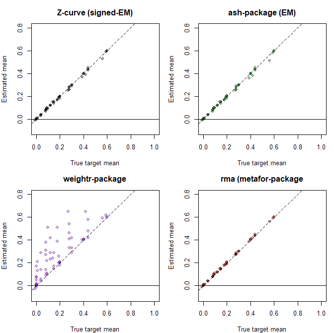
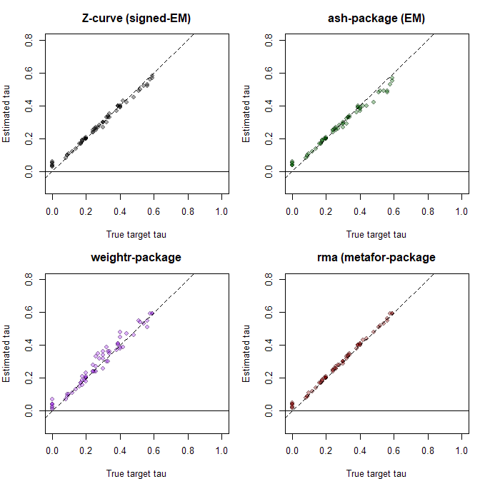
Correction (2026-07-14) The original post claimed that violations of the normality assumption biases standard random effects estimates. That finding was based on a coding error in the simulation program. The revised post shows the results for simulations with normal distributed effect sizes for H1 and mixtures of H0 and H1. In these simulations only estimates of the weight-function selection model (weightr package) are biased when the unimodal normal distribution assumption is violated.
Introduction
The main purpose of meta-analysis is to combine the results of quantitative studies. The simplest form averages the effect-size estimates of studies. The average is a better estimate of the population effect size because it draws on the combined sample size of the individual studies, and larger samples have less sampling error. A more sophisticated version takes each study’s sampling error into account, weighting studies with larger samples more heavily than those with smaller samples. This weighted average approximates the estimate one would obtain by pooling the raw data, under the assumption that all studies estimate the same effect.
These so-called fixed-effect meta-analyses assume that the samples are all drawn from the same population and that studies used interchangeable procedures, so that they all estimate a single population effect size. This assumption is defensible for a few phenomena grounded in basic sensory or cognitive architecture. Weber’s law, for instance — that the just-noticeable difference between two stimuli is a roughly constant proportion of their magnitude — reflects a property of sensory transduction and varies little across procedures and individuals. But such near-constants are the exception. Most effects in psychology vary with situational and personality factors, within and across cultures. This variation adds real differences in the true effect sizes across studies, over and above sampling error.
In recognition of this true variation, statisticians developed random-effects models (DerSimonian & Laird, 1986). To model the variation in population effect sizes, it is necessary to select a model that describes the unobserved variation in population effect sizes. From a statistical perspective, the easiest model assumes that population effect sizes have a normal distribution. The symmetry of this assumption implies that the estimate obtained from a set of studies is an unbiased estimate of the true average because positive and negative deviations from the average population effect size cancel each other out, just like random sampling errors cancel each other out.
Distribution Assumptions
From a theoretical perspective, it is unlikely that population effect sizes are normally distributed, particularly when the mean effect is small relative to the between-study heterogeneity. The reason is that effects are typically coded so that positive values are consistent with a directional theoretical prediction (e.g., conflicting colors produce slower responses in the Stroop task). While the size of the effect may vary across studies, it is often implausible that the true effect in some studies would be reversed (that conflicting colors would genuinely speed responses). A normal distribution, however, has support over the entire range of effect sizes and therefore always assigns some probability to negative true effects — an implication that is difficult to justify for a directionally predicted effect. When the mean is small relative to the heterogeneity, a normal distribution implies that a non-trivial proportion of true effects are negative, which is often theoretically implausible.
In practice, however, when heterogeneity is small, violations of the normality assumption have small and often negligible effects on meta-analytic estimates of the average effect (Hedges & Vevea, 1996). This helps explain why widely used random-effects models share the assumption that population effect sizes are normally distributed, including standard random-effects meta-analysis (DerSimonian & Laird, 1986) as implemented in commonly used software (Viechtbauer, 2010), selection-model approaches (Vevea & Hedges, 1995; Vevea & Woods, 2005), and the random-effects components of Bayesian model-averaging methods (Bartoš et al., 2023; Maier et al., 2023).
Necessary and Unnecessary Assumptions
It is useful to distinguish between necessary and unnecessary assumptions. All statistical methods require some assumptions to reduce the complex information in data to an interpretable statistic. However, not all assumptions of a model are necessary. In general, models with fewer unnecessary assumptions are preferable because they are robust to violations of these unnecessary assumptions by design. For example, the Pearson correlation coefficient assumes normal distribution of the two variables, whereas rank-order correlations do not. This makes rank-order correlations robust to violations of the normal distribution assumption and it is common practice to prefer rank-order correlations when variables’ distributions are not normal.
In meta-analyses, the assumption that population effect sizes are normally distributed is an unnecessary assumption. The idea of estimating the distribution of effects without assuming a parametric form is not new. Laird (1978) and Lindsay (1983) showed that the mixing distribution in a mixture model can be estimated nonparametrically by maximum likelihood, and that the resulting estimate takes the form of a discrete distribution on a finite set of support points. This provided, in principle, a fully flexible way to model heterogeneity without assuming normality. In practice, however, fitting these models was computationally demanding at the time.
Advances in optimization and computing have since removed these hurdles. Efficient algorithms for estimating mixture models — including modern convex-optimization methods (Koenker & Mizera, 2014; Kim et al., 2020) — now make it possible to fit flexible mixtures quickly and reliably. These developments led to the widespread adoption of nonparametric and empirical-Bayes mixture models in fields that analyze large numbers of effects, most notably genomics (Efron, 2010; Stephens, 2017), where the goal is to characterize the distribution of effects across thousands of tests and to identify which are likely to be real. Similar approaches have been applied in astronomy, education, and other areas that deal with many parallel estimates.
Heterogeneity of Population Effect Sizes
Meta-analysis, however, did not adopt these models, and continued to rely on the normal random-effects model. One reason is that the goal of most meta-analyses has been to estimate a single average effect, for which the shape of the effect-size distribution is largely irrelevant. The additional information provided by a flexible mixture — the structure of the heterogeneity itself — was not part of the question being asked.
This has changed with growing recognition of the distinction between direct and conceptual replication (Zwaan et al., 2018). Experimental psychologists rarely repeat a procedure exactly. Instead, they typically vary paradigms across studies in the belief that this is good scientific practice — probing moderators, boundary conditions, and the generalizability of an effect. As a result, the studies combined in a meta-analysis often estimate genuinely different population effects, and meta-analyses of such conceptual replications frequently show high estimates of heterogeneity (van Erp et al., 2017). In these cases the average effect size is of relatively minor interest, because it merely centers a wide distribution of different population effect sizes — an average across paradigm variants that no single study actually instantiates. The scientifically interesting question is not the average, but how and why the effects differ.
Mixture Models
Mixture models have another advantage over random effects models for meta-analysis. In standard meta-analytic models the population distribution of effect sizes is characterized by the mean and standard deviation of a normal distribution. Importantly, this information is removed from the observed data. It is therefore not possible to use this information to make sense of the heterogeneity in the observed effect size estimates in the data. A large effect size in the data may correspond to a small population effect size because it was inflated by sampling error and vice versa. This explains why heterogeneity often plays a minor role in the interpretation of meta-analyses. Heterogeneity exists, but it cannot be explained.
In contrast, mixture models combined with statistical tools that correct for regression to the mean make it possible to obtain estimates of the population effect size of individual studies. Often these effect size estimates for single studies have large uncertainty (wide confidence intervals), but they can be averaged to identify subgroups of studies with large effect sizes. This makes it possible to explore the heterogeneity in observed studies.
Simulation Study
To demonstrate the capabilities and advantages of mixture models over traditional random-effects models, I conducted a simulation study. To isolate the effect of the distributional assumption, the simulation used unbiased data (no publication selection). This removes selection as a confound and allows inclusion of the adaptive-shrinkage mixture model ash (Stephens, 2017), which was developed for genomics and assumes complete, unselected data. The other two models — the weight-function selection model (Vevea & Woods, 2005) and z-curve — model publication bias but reduce to unbiased estimation when no selection is present.
Z-curve is a meta-analytic mixture model (Brunner & Schimmack, 2020; Bartoš & Schimmack, 2022). Version 1 used the noncentrality parameters (ncp) of significant results to estimate the expected replication rate for direct replication studies. Version 2 used the ncp distribution across all studies to estimate the expected discovery rate. Version 3 adds an empirical-Bayes function that estimates population effect sizes by multiplying ncp estimates by their corresponding sampling errors, recovering effects from the latent distribution of noncentrality parameters.
The simulation used fixed sample sizes across studies, which ensures that mixture models fit in the effect-size metric and in the ncp metric produce identical results. Each condition contained k = 1,000 studies; the large k yields small sampling error in the estimates, making systematic biases more visible. The design crossed 4 means and 4 standard deviations of the population effect-size distribution with 4 proportions of true null hypotheses, producing 64 conditions. The population effect sizes when H1 is true were drawn from a normal distribution. However, mixing true H0 and H1 produces non-normal, bimodal distributions. This violates the distribution assumption of standard meta-analytic methods and could produce biased estimates.
These results for the mixture models (z-curve, ash) are not surprising. The models make no distribution assumptions and estimates of the mean closely match the simulated true values (z-curve RMSE = .009; ash RMSE = .010). The weight-function selection model had worse fit (RMSE = .138), but the random effects model fit as well as the mixture models (RMA RMSE = .003).
The results for the estimate of heterogeneity (tau) showed that all models estimated heterogeneity well, (z-curve RMSE = .018, ash RMSE = .027, weightr RMSE = .030, RMA RMSE = .013).
The present results show that the random effects model is robust to violations of the normality assumption even when heterogeneity is large and distributions are bimodal. The same cannot be said for the selection model with a normal assumption (weightr). Here the weight parameters to model selection bias can be biased to fit a normal distribution to non-normal observed data. The main implication is that it is possible to improve the performance of selection models by avoiding the normality assumption and modeling the distribution of population effect sizes with a flexible mixture model.
Implications
The present simulation showed that the random-effects model estimates the mean effect well when data are unbiased, even when its distributional assumptions are violated. This is consistent with a substantial prior literature. Simulation studies have repeatedly found that the pooled mean from the normal random-effects model is robust to non-normal random-effects distributions, including skewed and mixture distributions (Yamaguchi et al., 2017; Rubio-Aparicio et al., 2023; Baur et al., 2025). The robustness follows from the estimator itself: the pooled mean is an inverse-variance weighted average, which is consistent for the population mean regardless of the shape of the effect distribution. Large numbers of studies further protect against non-normality (Rubio-Aparicio et al., 2023), and with k = 1,000 the present simulation is in this favorable regime.
Where the normality assumption does matter is not the mean but the characterization of the distribution around it. The same literature finds that non-normality degrades the coverage of confidence and prediction intervals far more than it biases the mean (Baur et al., 2025), and that a symmetric normal model produces a wrongly symmetric prediction interval and a misleading heterogeneity summary when the true distribution is skewed (Yamaguchi et al., 2017). The recognized advantage of flexible mixture and semi-parametric models is therefore not lower bias on the mean but their ability to reveal latent structure — clusters and subgroups of studies — that the mean and a single heterogeneity parameter discard (Baur et al., 2025).
These are real but secondary limitations. The more fundamental problem is one that no distributional flexibility can address: the random-effects model, and the adaptive-shrinkage mixture model (ash) alike, assume that the observed studies are an unbiased sample of the population. In many literatures this assumption is untenable. In psychology, studies with significant results are far more likely to be published; the proportion of significant results often exceeds 90% (Sterling et al., 1995). Such publication bias inflates effect-size estimates, and correcting for it requires modeling the selection process — something neither the random-effects model nor ash attempts. A flexible distribution alone is not enough; what is needed is a model that combines distributional flexibility with a model of selection.
Z-curve occupies this niche: it combines a selection model, which corrects for publication bias, with a flexible mixture model, which captures heterogeneity without a distributional assumption. This is why z-curve outperforms weight-function models when studies are both heterogeneous and affected by publication bias (Schimmack, 2026).
References:
Bartoš, F., Maier, M., Wagenmakers, E.-J., Doucouliagos, H., & Stanley, T. D. (2023). Robust Bayesian meta-analysis: Model-averaging across complementary publication bias adjustment methods. Research Synthesis Methods, 14(1), 99–116.
Böhning, D. (2000). Computer-assisted analysis of mixtures and applications: Meta-analysis, disease mapping and others. Chapman & Hall/CRC.
DerSimonian, R., & Laird, N. (1986). Meta-analysis in clinical trials. Controlled Clinical Trials, 7(3), 177–188.
Hedges, L. V., & Vevea, J. L. (1996). Estimating effect size under publication bias: Small sample properties and robustness of a random effects selection model. Journal of Educational and Behavioral Statistics, 21(4), 299–332.
Laird, N. (1978). Nonparametric maximum likelihood estimation of a mixing distribution. Journal of the American Statistical Association, 73(364), 805–811.
Lindsay, B. G. (1983). The geometry of mixture likelihoods: A general theory. The Annals of Statistics, 11(1), 86–94.
Maier, M., Bartoš, F., & Wagenmakers, E.-J. (2023). Robust Bayesian meta-analysis: Addressing publication bias with model-averaging. Psychological Methods, 28(1), 107–122.
Stephens, M. (2017). False discovery rates: A new deal. Biostatistics, 18(2), 275–294.
Vevea, J. L., & Hedges, L. V. (1995). A general linear model for estimating effect size in the presence of publication bias. Psychometrika, 60(3), 419–435.
Vevea, J. L., & Woods, C. M. (2005). Publication bias in research synthesis: Sensitivity analysis using a priori weight functions. Psychological Methods, 10(4), 428–443.
Viechtbauer, W. (2010). Conducting meta-analyses in R with the metafor package. Journal of Statistical Software, 36(3), 1–48.
Efron, B. (2010). Large-scale inference: Empirical Bayes methods for estimation, testing, and prediction. Cambridge University Press.
Kim, Y., Carbonetto, P., Stephens, M., & Koenker, R. (2020). A fast algorithm for maximum likelihood estimation of mixture proportions using sequential quadratic programming. Journal of Computational and Graphical Statistics, 29(2), 261–273.
Koenker, R., & Mizera, I. (2014). Convex optimization, shape constraints, compound decisions, and empirical Bayes rules. Journal of the American Statistical Association, 109(506), 674–685.
Laird, N. (1978). Nonparametric maximum likelihood estimation of a mixing distribution. Journal of the American Statistical Association, 73(364), 805–811.
Lindsay, B. G. (1983). The geometry of mixture likelihoods: A general theory. The Annals of Statistics, 11(1), 86–94.
The pattern is now familiar. I received another anonymous review by Reviewer 2 from a z-curve article that repeated Pek’s concerns about the performance of z-curve. To deal with biased reviewers, journals allow authors to mention potentially biased reviewers. I suggest doing so for Pek. I also suggest sharing a manuscript with me to ensure proper interpretation of results and to make it “reviewer-safe.”
To justify the claim that Pek is biased, researchers can use this rebuttal of Pek’s unscientific claims about z-curve.
Reviewer 2
Reviewer Report:
The manuscript “A review and z-curve analysis of research on the palliative association of system justification” (Manuscript ID 1598066) extends the work of Sotola and Credé (2022), who used Z-curve analysis to evaluate the evidential value of findings related to system justification theory (SJT). The present paper similarly reports estimates of publication bias, questionable research practices (QRPs), and replication rates in the SJT literature using Z-curve. Evaluating how scientific evidence accumulates in the published literature is unquestionably important.
However, there is growing concern about the performance of meta-analytic forensic tools such as p-curve (Simonsohn, Nelson, & Simmons, 2014; see Morey & Davis-Stober, 2025 for a critique) and Z-curve (Brunner & Schimmack, 2020; Bartoš & Schimmack, 2022; see Pek et al., in press for a critique). Independent simulation studies increasingly suggest that these methods may perform poorly under realistic conditions, potentially yielding misleading results.
Justification for a theory or method typically requires subjecting it to a severe test (Mayo, 2019) – that is, assuming the opposite of what one seeks to establish (e.g., a null hypothesis of no effect) and demonstrating that this assumption leads to contradiction. In contrast, the simulation work used to support Z-curve (Brunner & Schimmack, 2020; Bartoš & Schimmack, 2022) relies on affirming belief through confirmation, a well-documented cognitive bias.
Findings from Pek et al. (in press) show that when selection bias is presented in published p-values — the very scenario Z-curve was intended to be applied — estimates of the expected discovery rate (EDR), expected replication rate (ERR), and Sorić’s False Discovery Risk (FDR) are themselves biased.
The magnitude and direction of this bias depend on multiple factors (e.g., number of p-values, selection mechanism of p-values) and cannot be corrected or detected from empirical data alone. The manuscript’s main contribution rests on the assumption that Z-curve yields reasonable estimates of the “reliability of published studies,” operationalized as a high ERR, and that the difference between the observed discovery rate (ODR) and EDR quantifies the extent of QRPs and publication bias.
The paper reports an ERR of .76, 95% CI [.53, .91] and concludes that research on the palliative hypothesis may be more reliable than findings in many other areas of psychology. There are several issues with this claim. First, the assertion that Sotola (2023) validated ERR estimates from the Z-curve reflects confirmation bias – I have not read Röseler (2023) and cannot comment on the argument made in it. The argument rests solely on the descriptive similarly between the ERR produced by Z-curve and the replication rate reported by the Open Science Collaboration (2015). However, no formal test of equivalence was conducted, and no consideration was given to estimate imprecision, potential bias in the estimates, or the conditions under which such agreement might occur by chance.
At minimum, if Z-curve estimates are treated as predicted values, some form of cross-validation or prediction interval should be used to quantify prediction uncertainty. More broadly, because ERR estimates produced by Z-curve are themselves likely biased (as shown in Pek et al., in press), and because the magnitude and direction of this bias are unknown, comparisons about ERR values across literatures do not provide a strong evidential basis for claims about the relative reliability of research areas.
Furthermore, the width of the 95% CI spans roughly half of the bounded parameter space of [0, 1], indicating substantial imprecision. Any claims based on these estimates should thus be contextualized with appropriate caution.
Another key result concerns the comparison of EDR = .52, 95% CO [.14, .92], and ODR = .81, 95% CI = [.69, .90]. The manuscript states that “When these two estimates are highly discrepant, this is consistent with the presence of questionable research practices (QRPS) and publication bias in this area of research (Brunner & Schimmack, 2020).
But in this case, the 95% CIs for the EDR and ODR in this work overlapped quite a bit, meaning that they may not be significantly different…” (p. 22). There are several issues with such a claim. First, Z curve results cannot directly support claims about the presence of QRPs.
The EDR reflects the proportion of significant p values expected under no selection bias, but it does not identify the source of selection bias (e.g., QRPs, fraud, editorial decisions). Using Z curve requires accepting its assumed missing data mechanism—a strong assumption that cannot be empirically validated.
Second, a descriptive comparison between two estimates cannot be interpreted as a formal test of difference (e.g., eyeballing two estimates of means as different does not tell us whether this difference is not driven by sampling variability). Means can be significantly different even if their confidence intervals overlap (Cumming & Finch, 2005).
A formal test of the difference is required. Third, EDR estimates can be biased. Even under ideal conditions, convergence to the population values requires extremely large numbers of studies (e.g., > 3000, see Figure 1 of Pek et al., in press).
The current study only has 64 tests. Thus, even if a formal test of the difference of ODR – EDR was conducted, little confidence could be placed on the result if the EDR estimate is biased and does not reflect the true population value.
Although I am critical of the outputs of Z curve analysis due to its poor statistical performance under realistic conditions, the manuscript has several strengths. These include adherence to good meta analytic practices such as providing a PRISMA flow chart, clearly stating inclusion and exclusion criteria, and verifying the calculation of p values. These aspects could be further strengthened by reporting test–retest reliability (given that a single author coded all studies) and by explicitly defining the population of selected p values. Because there appears to be heterogeneity in the results, a random effects meta analysis may be appropriate, and study level variables (e.g., type of hypothesis or analysis) could be used to explain between study variability. Additionally, the independence of p values has not been clearly addressed; p values may be correlated within articles or across studies. Minor points: The “reliability” of studies should be explicitly defined. The work by Manapat et al. (2022) should be cited in relation to Nagy et al. (2025). The findings of Simmons et al. (2011) applies only to single studies.
However, most research is published in multi-study sets, and follow-up simulations by Wegener at al. (2024) indicate that the Type I error rate is well-controlled when methodological constraints (e.g., same test, same design, same measures) are applied consistently across multiple studies – thus, the concerns of Simmons et al. (2011) pertain to a very small number of published results.
I could not find the reference to Schimmack and Brunner (2023) cited on p. 17.
Rebuttal to Core Claims in Recent Critiques of z-Curve
1. Claim: z-curve “performs poorly under realistic conditions”
Rebuttal
The claim that z-curve “performs poorly under realistic conditions” is not supported by the full body of available evidence. While recent critiques demonstrate that z-curve estimates—particularly EDR—can be biased under specific data-generating and selection mechanisms, these findings do not justify a general conclusion of poor performance.
Z-curve has been evaluated in extensive simulation studies that examined a wide range of empirically plausible scenarios, including heterogeneous power distributions, mixtures of low- and high-powered studies, varying false-positive rates, different degrees of selection for significance, and multiple shapes of observed z-value distributions (e.g., unimodal, right-skewed, and multimodal distributions). These simulations explicitly included sample sizes as low as k ≈ 100, which is typical for applied meta-research in psychology.
Across these conditions, z-curve demonstrated reasonable statistical properties conditional on its assumptions, including interpretable ERR and EDR estimates and confidence intervals with acceptable coverage in most realistic regimes. Importantly, these studies also identified conditions under which estimation becomes less informative—such as when the observed z-value distribution provides little information about missing nonsignificant results—thereby documenting diagnosable scope limits rather than undifferentiated poor performance.
Recent critiques rely primarily on selective adversarial scenarios and extrapolate from these to broad claims about “realistic conditions,” while not engaging with the earlier simulation literature that systematically evaluated z-curve across a much broader parameter space. A balanced scientific assessment therefore supports a more limited conclusion: z-curve has identifiable limitations and scope conditions, but existing simulation evidence does not support the claim that it generally performs poorly under realistic conditions.
2. Claim: Bias in EDR or ERR renders these estimates uninterpretable or misleading
Rebuttal
The critique conflates the possibility of bias with a lack of inferential value. All methods used to evaluate published literatures under selection—including effect-size meta-analysis, selection models, and Bayesian hierarchical approaches—are biased under some violations of their assumptions. The existence of bias therefore does not imply that an estimator is uninformative.
Z-curve explicitly reports uncertainty through bootstrap confidence intervals, which quantify sampling variability and model uncertainty given the observed data. No evidence is presented that z-curve confidence intervals systematically fail to achieve nominal coverage under conditions relevant to applied analyses. The appropriate conclusion is that z-curve estimates must be interpreted conditionally and cautiously, not that they lack statistical meaning.
This claim overgeneralizes results from specific, highly constrained simulation scenarios. The cited sample sizes correspond to conditions in which the observed data provide little identifying information, not to a general requirement for statistical validity.
In applied statistics, consistency in the limit does not imply that estimates at smaller sample sizes are meaningless; it implies that uncertainty must be acknowledged. In the present application, this uncertainty is explicitly reflected in wide confidence intervals. Small sample sizes therefore affect precision, not validity, and do not justify dismissing the estimates outright.
4. Claim: Differences between ODR and EDR cannot support inferences about selection or questionable research practices
Rebuttal
It is correct that differences between ODR and EDR do not identify the source of selection (e.g., QRPs, editorial decisions, or other mechanisms). However, the critique goes further by implying that such differences lack diagnostic value altogether.
Under the z-curve framework, ODR–EDR discrepancies are interpreted as evidence of selection, not of specific researcher behaviors. This inference is explicitly conditional and does not rely on attributing intent or mechanism. Rejecting this interpretation would require demonstrating that ODR–EDR differences are uninformative even under monotonic selection on statistical significance, which has not been shown.
5. Claim: ERR comparisons across literatures lack evidential basis because bias direction is unknown
Rebuttal
The critique asserts that because ERR estimates may be biased with unknown direction, comparisons across literatures lack evidential value. This conclusion does not follow.
Bias does not eliminate comparative information unless it is shown to be large, variable, and systematically distorting rankings across plausible conditions. No evidence is provided that ERR estimates reverse ordering across literatures or are less informative than alternative metrics. While comparative claims should be interpreted cautiously, caution does not imply the absence of evidential content.
6. Claim: z-curve validation relies on “affirming belief through confirmation”
Rebuttal
This characterization misrepresents the role of simulation studies in statistical methodology. Simulation-based evaluation of estimators under known data-generating processes is the standard approach for assessing bias, variance, and coverage across frequentist and Bayesian methods alike.
Characterizing simulation-based validation as epistemically deficient would apply equally to conventional meta-analysis, selection models, and hierarchical Bayesian approaches. No alternative validation framework is proposed that would avoid reliance on model-based simulation.
7. Implicit claim: Effect-size meta-analysis provides a firmer basis for credibility assessment
Rebuttal
Effect-size meta-analysis addresses a different inferential target. It presupposes that studies estimate commensurable effects of a common hypothesis. In heterogeneous literatures, pooled effect sizes represent averages over substantively distinct estimands and may lack clear interpretation.
Moreover, effect-size meta-analysis does not estimate discovery rates, replication probabilities, or false-positive risk, nor does it model selection unless explicitly extended. No evidence is provided that effect-size meta-analysis offers superior performance for evaluating evidential credibility under selective reporting.
Summary
The critiques correctly identify that z-curve is a model-based method with assumptions and scope conditions. However, they systematically extend these points beyond what the evidence supports by:
extrapolating from selective adversarial simulations,
conflating potential bias with lack of inferential value,
overgeneralizing small-sample limitations,
and applying asymmetrical standards relative to conventional methods.
A scientifically justified conclusion is that z-curve provides conditionally informative estimates with quantifiable uncertainty, not that it lacks statistical validity or evidential relevance.
This is the final version of our response to Pek et al.’s criticism of z-curve in Cognition and Emotion that is now accepted for publication. I share it here as the actual response is hidden behind a paywall. To cite this content, use the following official citation:
Schimmack, U., & Soto, M. D. (2026). A response to Pek et al.’s commentary on Z-curve: clarifying the assumptions of selection models. Cognition and Emotion, 1–5. https://doi.org/10.1080/02699931.2026.2678998
Abstract
Pek et al. (2026) comment on Soto and Schimmack (2025) and raise concerns about the use of z-curve to evaluate the credibility of emotion research. Their central criticism is based on simulations showing that z-curve can overestimate the expected discovery rate when selection operates not only at the level of statistical significance but also within the set of significant results as a function of effect size. This point is correct: if researchers selectively publish larger significant effects while suppressing smaller significant ones, selection models that assume threshold-based filtering can be biased. However, this limitation is not unique to z-curve and applies equally to other selection models used in meta-analysis. More importantly, there is currently little empirical evidence for effect-size bias, while there is ample evidence of selection based on significance. Under these more realistic conditions, z-curve provides informative estimates of (a) selection bias, (b) the expected replication rate, and (c) the false positive risk. Our results also demonstrate substantial inflation of effect size estimates in traditional meta-analyses that ignore selection processes. For these reasons, we reject the recommendation to rely solely on standard meta-analytic approaches and advocate for the use of selection models to obtain more realistic estimates.
The z-curve analysis of results in this journal shows (a) that many published results are based on studies with low to modest power, (b) selection for significance inflates effect size estimates and the discovery rate of reported results, and (c) there is no evidence that research practices have changed over the past decade. Readers should be careful when they interpret results and recognize that reported effect sizes are likely to overestimate real effect sizes, and that replication studies with the same sample size may fail to produce a significant result again. To avoid misleading inferences, I suggest using alpha = .005 as a criterion for valid rejections of the null-hypothesis. Using this criterion, the risk of a false positive result is below 2%. I also recommend computing a 99% confidence interval rather than the traditional 95% confidence interval for the interpretation of effect size estimates.
Given the low power of many studies, readers also need to avoid the fallacy to report non-significant results as evidence for the absence of an effect. With 50% power, the results can easily switch in a replication study so that a significant result becomes non-significant and a non-significant result becomes significant. However, selection for significance will make it more likely that significant results become non-significant than observing a change in the opposite direction.
The average power of studies in a heterogeneous journal like Frontiers of Psychology provides only circumstantial evidence for the evaluation of results. When other information is available (e.g., z-curve analysis of a discipline, author, or topic, it may be more appropriate to use this information).
Report
Frontiers of Psychology was created in 2010 as a new online-only journal for psychology. It covers many different areas of psychology, although some areas have specialized Frontiers journals like Frontiers in Behavioral Neuroscience.
The business model of Frontiers journals relies on publishing fees of authors, while published articles are freely available to readers.
The number of articles in Frontiers of Psychology has increased quickly from 131 articles in 2010 to 8,072 articles in 2022 (source Web of Science). With over 8,000 published articles Frontiers of Psychology is an important outlet for psychological researchers to publish their work. Many specialized, print-journals publish fewer than 100 articles a year. Thus, Frontiers of Psychology offers a broad and large sample of psychological research that is equivalent to a composite of 80 or more specialized journals.
Another advantage of Frontiers of Psychology is that it has a relatively low rejection rate compared to specialized journals that have limited journal space. While high rejection rates may allow journals to prioritize exceptionally good research, articles published in Frontiers of Psychology are more likely to reflect the common research practices of psychologists.
To examine the replicability of research published in Frontiers of Psychology, I downloaded all published articles as PDF files, converted PDF files to text files, and extracted test-statistics (F, t, and z-tests) from published articles. Although this method does not capture all published results, there is no a priori reason that results reported in this format differ from other results. More importantly, changes in research practices such as higher power due to larger samples would be reflected in all statistical tests.
As Frontiers of Psychology only started shortly before the replication crisis in psychology increased awareness about the problem of low statistical power and selection for significance (publication bias), I was not able to examine replicability before 2011. I also found little evidence of changes in the years from 2010 to 2015. Therefore, I use this time period as the starting point and benchmark for future years.
Figure 1 shows a z-curve plot of results published from 2010 to 2014. All test-statistics are converted into z-scores. Z-scores greater than 1.96 (the solid red line) are statistically significant at alpha = .05 (two-sided) and typically used to claim a discovery (rejection of the null-hypothesis). Sometimes even z-scores between 1.65 (the dotted red line) and 1.96 are used to reject the null-hypothesis either as a one-sided test or as marginal significance. Using alpha = .05, the plot shows 71% significant results, which is called the observed discovery rate (ODR).
Visual inspection of the plot shows a peak of the distribution right at the significance criterion. It also shows that z-scores drop sharply on the left side of the peak when the results do not reach the criterion for significance. This wonky distribution cannot be explained with sampling error. Rather it shows a selective bias to publish significant results by means of questionable practices such as not reporting failed replication studies or inflating effect sizes by means of statistical tricks. To quantify the amount of selection bias, z-curve fits a model to the distribution of significant results and estimates the distribution of non-significant (i.e., the grey curve in the range of non-significant results). The discrepancy between the observed distribution and the expected distribution shows the file-drawer of missing non-significant results. Z-curve estimates that the reported significant results are only 31% of the estimated distribution. This is called the expected discovery rate (EDR). Thus, there are more than twice as many significant results as the statistical power of studies justifies (71% vs. 31%). Confidence intervals around these estimates show that the discrepancy is not just due to chance, but active selection for significance.
Using a formula developed by Soric (1989), it is possible to estimate the false discovery risk (FDR). That is, the probability that a significant result was obtained without a real effect (a type-I error). The estimated FDR is 12%. This may not be alarming, but the risk varies as a function of the strength of evidence (the magnitude of the z-score). Z-scores that correspond to p-values close to p =.05 have a higher false positive risk and large z-scores have a smaller false positive risk. Moreover, even true results are unlikely to replicate when significance was obtained with inflated effect sizes. The most optimistic estimate of replicability is the expected replication rate (ERR) of 69%. This estimate, however, assumes that a study can be replicated exactly, including the same sample size. Actual replication rates are often lower than the ERR and tend to fall between the EDR and ERR. Thus, the predicted replication rate is around 50%. This is slightly higher than the replication rate in the Open Science Collaboration replication of 100 studies which was 37%.
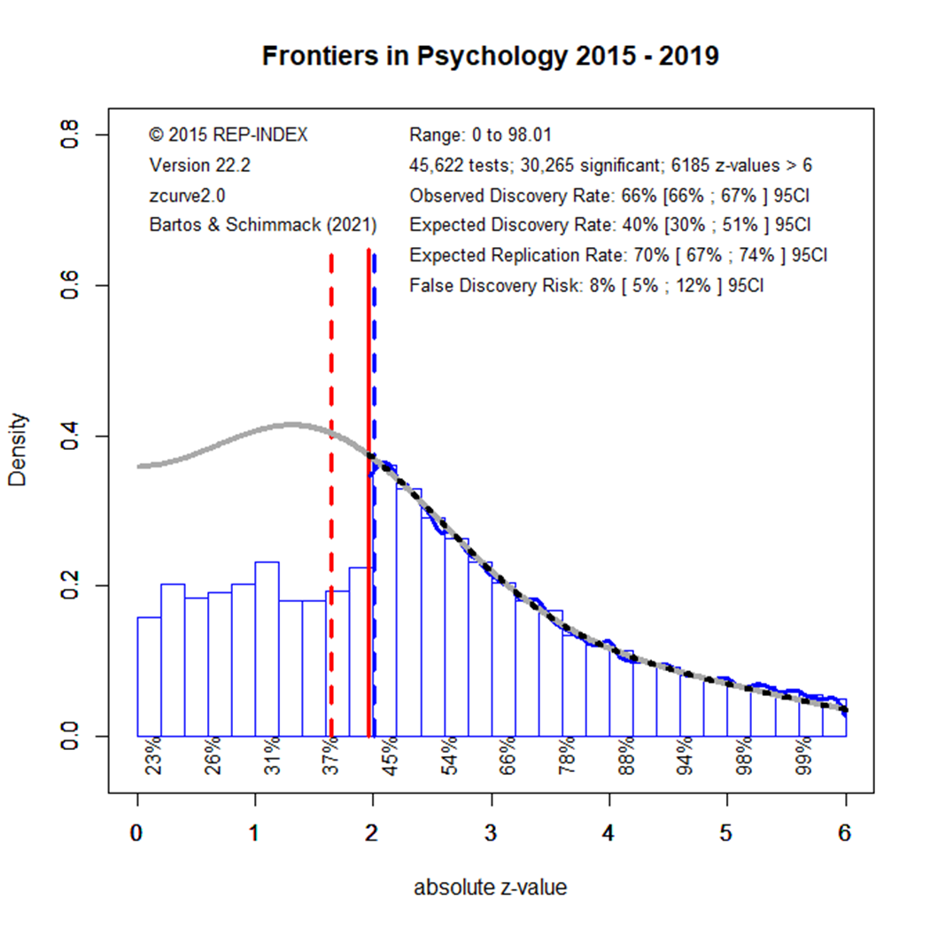
Figure 2 examines how things have changed in the next five years.
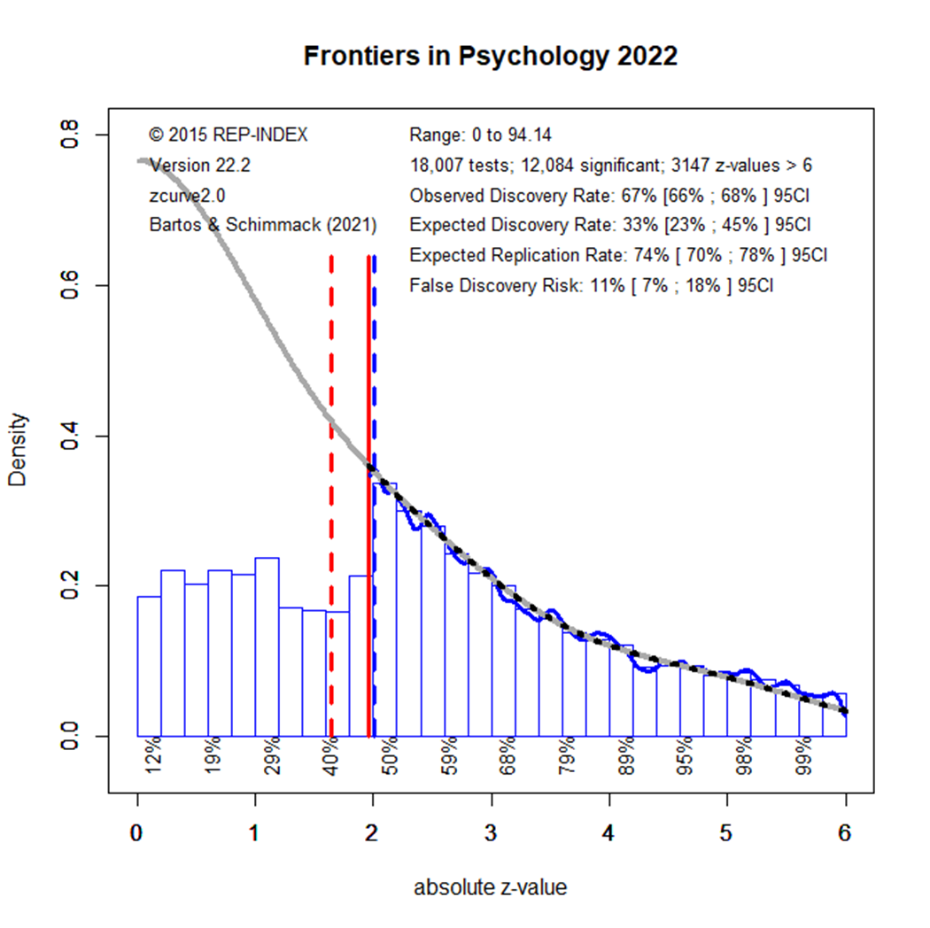
The observed discovery rate decreased slightly, but statistically significantly, from 71% to 66%. This shows that researchers reported more non-significant results. The expected discovery rate increased from 31% to 40%, but the overlapping confidence intervals imply that this is not a statistically significant increase at the alpha = .01 level. (if two 95%CI do not overlap, the difference is significant at around alpha = .01). Although smaller, the difference between the ODR of 60% and the EDR of 40% is statistically significant and shows that selection for significance continues. The ERR estimate did not change, indicating that significant results are not obtained with more power. Overall, these results show only modest improvements, suggesting that most researchers who publish in Frontiers in Psychology continue to conduct research in the same way as they did before, despite ample discussions about the need for methodological reforms such as a priori power analysis and reporting of non-significant results.
The results for 2020 show that the increase in the EDR was a statistical fluke rather than a trend. The EDR returned to the level of 2010-2015 (29% vs. 31), but the ODR remained lower than in the beginning, showing slightly more reporting of non-significant results. The size of the file drawer remains large with an ODR of 66% and an EDR of 72%.
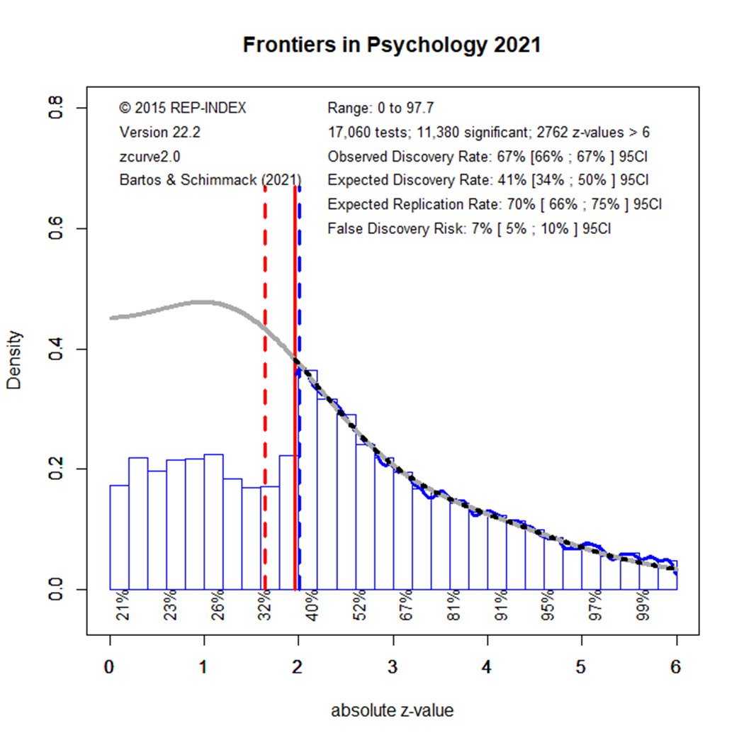
The EDR results for 2021 look again better, but the difference to 2020 is not statistically significant. Moreover, the results in 2022 show a lower EDR that matches the EDR in the beginning.
Overall, these results show that results published in Frontiers in Psychology are selected for significance. While the observed discovery rate is in the upper 60%s, the expected discovery rate is around 35%. Thus, the ODR is nearly twice the rate of the power of studies to produce these results. Most concerning is that a decade of meta-psychological discussions about research practices has not produced any notable changes in the amount of selection bias or the power of studies to produce replicable results.
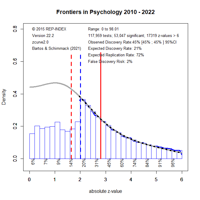
How should readers of Frontiers in Psychology articles deal with this evidence that some published results were obtained with low power and inflated effect sizes that will not replicate? One solution is to retrospectively change the significance criterion. Comparisons of the evidence in original studies and replication outcomes suggest that studies with a p-value below .005 tend to replicate at a rate of 80%, whereas studies with just significant p-values (.050 to .005) replicate at a much lower rate (Schimmack, 2022). Demanding stronger evidence also reduces the false positive risk. This is illustrated in the last figure that uses results from all years, given the lack of any time trend.
In the Figure the red solid line moved to z = 2.8; the value that corresponds to p = .005, two-sided. Using this more stringent criterion for significance, only 45% of the z-scores are significant. Another 25% were significant with alpha = .05, but are no longer significant with alpha = .005. As power decreases when alpha is set to more stringent, lower, levels, the EDR is also reduced to only 21%. Thus, there is still selection for significance. However, the more effective significance filter also selects for more studies with high power and the ERR remains at 72%, even with alpha = .005 for the replication study. If the replication study used the traditional alpha level of .05, the ERR would be even higher, which explains the finding that the actual replication rate for studies with p < .005 is about 80%.
The lower alpha also reduces the risk of false positive results, even though the EDR is reduced. The FDR is only 2%. Thus, the null-hypothesis is unlikely to be true. The caveat is that the standard null-hypothesis in psychology is the nil-hypothesis and that the population effect size might be too small to be of practical significance. Thus, readers who interpret results with p-values below .005 should also evaluate the confidence interval around the reported effect size, using the more conservative 99% confidence interval that correspondence to alpha = .005 rather than the traditional 95% confidence interval. In many cases, this confidence interval is likely to be wide and provide insufficient information about the strength of an effect.
Citation and link to the actual article: Bartoš, F. & Schimmack, U. (2022). Z‑curve 2.0: Estimating replication rates and discovery rates. Meta‑Psychology, Volume 6, Issue 4, Article MP.2021.2720. Published September 1, 2022. DOI:https://doi.org/10.15626/MP.2021.2720
Update July 14, 2021
After trying several traditional journals that are falsely considered to be prestigious because they have high impact factors, we are proud to announce that our manuscript “Z-curve 2.0: : Estimating Replication Rates and Discovery Rates” has been accepted for publication in Meta-Psychology. We received the most critical and constructive comments of our manuscript during the review process at Meta-Psychology and are grateful for many helpful suggestions that improved the clarity of the final version. Moreover, the entire review process is open and transparent and can be followed when the article is published. Moreover, the article is freely available to anybody interested in Z-Curve.2.0, including users of the zcurve package (https://cran.r-project.org/web/packages/zcurve/index.html).
Although the article will be freely available on the Meta-Psychology website, the latest version of the manuscript is posted here as a blog post. Supplementary materials can be found on OSF (https://osf.io/r6ewt/)
Z-curve 2.0: Estimating Replication and Discovery Rates
František Bartoš1,2,*, Ulrich Schimmack3 1 University of Amsterdam 2 Faculty of Arts, Charles University 3 University of Toronto, Mississauga
Correspondence concerning this article should be addressed to: František Bartoš, University of Amsterdam, Department of Psychological Methods, Nieuwe Achtergracht 129-B, 1018 VZ Amsterdam, The Netherlands, fbartos96@gmail.com
Submitted to Meta-Psychology. Participate in open peer review by commenting through hypothes.is directly on this preprint. The full editorial process of all articles under review at Meta-Psychology can be found following this link: https://tinyurl.com/mp-submissions
You will find this preprint by searching for the first authors name.
Abstract
Selection for statistical significance is a well-known factor that distorts the published literature and challenges the cumulative progress in science. Recent replication failures have fueled concerns that many published results are false-positives. Brunner and Schimmack (2020) developed z-curve, a method for estimating the expected replication rate (ERR) – the predicted success rate of exact replication studies based on the mean power after selection for significance. This article introduces an extension of this method, z-curve 2.0. The main extension is an estimate of the expected discovery rate (EDR) – the estimate of a proportion that the reported statistically significant results constitute from all conducted statistical tests. This information can be used to detect and quantify the amount of selection bias by comparing the EDR to the observed discovery rate (ODR; observed proportion of statistically significant results). In addition, we examined the performance of bootstrapped confidence intervals in simulation studies. Based on these results, we created robust confidence intervals with good coverage across a wide range of scenarios to provide information about the uncertainty in EDR and ERR estimates. We implemented the method in the zcurve R package (Bartoš & Schimmack, 2020).
It has been known for decades that the published record in scientific journals is not representative of all studies that are conducted. For a number of reasons, most published studies are selected because they reported a theoretically interesting result that is statistically significant; p < .05 (Rosenthal & Gaito, 1964; Scheel, Schijen, & Lakens, 2021; Sterling, 1959; Sterling et al., 1995). This selective publishing of statistically significant results introduces a bias in the published literature. At the very least, published effect sizes are inflated. In the most extreme cases, a false-positive result is supported by a large number of statistically significant results (Rosenthal, 1979).
Some sciences (e.g., experimental psychology) tried to reduce the risk of false-positive results by demanding replication studies in multiple-study articles (cf. Wegner, 1992). However, internal replication studies provided a false sense of replicability because researchers used questionable research practices to produce successful internal replications (Francis, 2014; John, Lowenstein, & Prelec, 2012; Schimmack, 2012). The pervasive presence of publication bias at least partially explains replication failures in social psychology (Open Science Collaboration, 2015; Pashler & Wagenmakers, 2012, Schimmack, 2020); medicine (Begley & Ellis, 2012; Prinz, Schlange, & Asadullah 2011), and economics (Camerer et al., 2016; Chang & Li, 2015).
In meta-analyses, the problem of publication bias is usually addressed by one of the different methods for its detection and a subsequent adjustment of effect size estimates. However, many of them (Egger, Smith, Schneider, & Minder, 1997; Ioannidis and Trikalinos, 2007; Schimmack, 2012) perform poorly under conditions of heterogeneity (Renkewitz & Keiner, 2019), whereas others employ a meta-analytic model assuming that the studies are conducted on a single phenomenon (e.g., Hedges, 1992; Vevea & Hedges, 1995; Maier, Bartoš & Wagenmakers, in press). Moreover, while the aforementioned methods test for publication bias (return a p-value or a Bayes factor), they usually do not provide a quantitative estimate of selection bias. An exception would be the publication probabilities/ratios estimates from selection models (e.g., Hedges, 1992). Maximum likelihood selection models work well when the distribution of effect sizes is consistent with model assumptions, but can be biased when the distribution when the actual distribution does not match the expected distribution (e.g., Brunner & Schimmack, 2020; Hedges, 1992; Vevea & Hedges, 1995). Brunner and Schimmack (2020) introduced a new method that does not require a priori assumption about the distribution of effect sizes. The z-curve method uses a finite mixture model to correct for selection bias. We extended z-curve to also provide information about the amount of selection bias. To distinguish between the new and old z-curve methods, we refer to the old z-curve as z-curve 1.0 and the new z-curve as z-curve 2.0. Z-curve 2.0 has been implemented in the open statistic program R as the zcurve package that can be downloaded from CRAN (Bartoš & Schimmack, 2020).
Before we introduce z-curve 2.0, we would like to introduce some key statistical terms. We assume that readers are familiar with the basic concepts of statistical significance testing; normal distribution, null-hypothesis, alpha, type-I error, and false-positive result (see Bartoš & Maier, in press, for discussion of some of those concepts and their relation).
Glossary
Power is defined as the long-run relative frequency of statistically significant results in a series of exact replication studies with the same sample size when the null-hypothesis is false. For example, in a study with two groups (n = 50), a population effect size of Cohen’s d = 0.4 has 50.8% power to produce a statistically significant result. Thus, 100 replications of this study are expected to produce approximately 50 statistically significant results. The actual frequency will approach 50.8% as the study is repeated infinitely.
Unconditional power extends the concept of power to studies where the null-hypothesis is true. Typically, power is a conditional probability assuming a non-zero effect size (i.e., the null-hypothesis is false). However, the long-run relative frequency of statistically significant results is also known when the null-hypothesis is true. In this case, the long-run relative frequency is determined by the significance criterion, alpha. With alpha = 5%, we expect that 5 out of 100 studies will produce a statistically significant result. We use the term unconditional power to refer to the long-run frequency of statistically significant results without conditioning on a true effect. When the effect size is zero and alpha is 5%, unconditional power is 5%. As we only consider unconditional power in this article, we will use the term power to refer to unconditional power, just like Canadians use the term hockey to refer to ice hockey.
Mean (unconditional) power is a summary statistic of studies that vary in power. Mean power is simply the arithmetic mean of the power of individual studies. For example, two studies with power = .4 and power = .6, have a mean power of .5.
Discovery rate is a relative frequency of statistically significant results. Following Soric (1989), we call statistically significant results discoveries. For example, if 100 studies produce 36 statistically significant results, the discovery rate is 36%. Importantly, the discovery rate does not distinguish between true or false discoveries. If only false-positive results were reported, the discovery rate would be 100%, but none of the discoveries would reflect a true effect (Rosenthal, 1979).
Selection bias is a process that favors the publication of statistically significant results. Consequently, the published literature has a higher percentage of statistically significant results than was among the actually conducted studies. It results from significance testing that creates two classes of studies separated by the significance criterion alpha. Those with a statistically significant result, p < .05, where the null-hypothesis is rejected, and those with a statistically non-significant result, where the null-hypothesis is not rejected, p > .05. Selection for statistical significance limits the population of all studies that were conducted to the population of studies with statistically significant results. For example, if two studies produce p-values of .20 and .01, only the study with the p-value .01 is retained. Selection bias is often called publication bias. Studies show that authors are more likely to submit findings for publication when the results are statistically significant (Franco, Malhotra & Simonovits, 2014).
Observed discovery rate (ODR) is the percentage of statistically significant results in an observed set of studies. For example, if 100 published studies have 80 statistically significant results, the observed discovery rate is 80%. The observed discovery rate is higher than the true discovery rate when selection bias is present.
Expected discovery rate (EDR) is the mean power before selection for significance; in other words, the mean power of all conducted studies with statistically significant and non-significant results. As power is the long-run relative frequency of statistically significant results, the mean power before selection for significance is the expected relative frequency of statistically significant results. As we call statistically significant results discoveries, we refer to the expected percentage of statistically significant results as the expected discovery rate. For example, if we have two studies with power of .05 and .95, we are expecting 1 statistically significant result and an EDR of 50%, (.95 + .05)/2 = .5.
Expected replication rate (ERR) is the mean power after selection for significance, in other words, the mean power of only the statistically significant studies. Furthermore, since most people would declare a replication successful only if it produces a result in the same direction, we base ERR on the power to obtain a statistically significant result in the same direction. Using the prior example, we assume that the study with 5% power produced a statistically non-significant result and the study with 95% power produced a statistically significant result. In this case, we end up with only one statistically significant result with 95% power. Subsequently, the mean power after selection for significance is 95% (there is almost zero chance that a study with 95% power would produce replication with an outcome in the opposite direction). Based on this estimate, we would predict that 95% of exact replications of this study with the same sample size, and therefore with 95% power, will be statistically significant in the same direction.
As mean power after selection for significance predicts the relative frequency of statistically significant results in replication studies, we call it the expected replication rate. The ERR also corresponds to the “aggregate replication probability” discussed by Miller (2009).
Numerical Example
Before introducing the formal model, we illustrate the concepts with a fictional example. In the example, researchers test 100 true hypotheses with 100% power (i.e., every test of a true hypothesis produces p < .05) and 100 false hypotheses (H0 is true) with 5% power which is determined by alpha = .05. Consequently, the researchers obtain 100 true positive results and 5 false-positive results, for a total of 105 statistically significant results.[1] The expected discovery rate is (1 × 100 + 0.05 × 100)/(100 + 100) = 105/200 = 52.5% which corresponds to the observed discovery rate when all conducted studies are reported.
So far, we have assumed that there is no selection bias. However, let us now assume that 50 of the 95 statistically non-significant results are not reported. In this case, the observed discovery rate increased from 105/200 to 105/150 = 70%. The discrepancy between the EDR, 52.5%, and the ODR, 70%, provides quantitative information about the amount of selection bias.
As shown, the EDR provides valuable information about the typical power of studies and about the presence of selection bias. However, it does not provide information about the replicability of the statistically significant results. The reason is that studies with higher power are more likely to produce a statistically significant result in replications (Brunner & Schimmack, 2020; Miller, 2009). The main purpose of z-curve 1.0 was to estimate the mean power after selection for significance to predict the outcome of exact replication studies. In the example, only 5 of the 100 false hypotheses were statistically significant. In contrast, all 100 tests of the true hypothesis were statistically significant. This means that the mean power after selection for significance is (5 × .025 + 100 × 1)/(5 + 100) = 100.125/105 ≈ 95.4%, which is the expected replication rate.
Formal Introduction
Unfortunately, there is no standard symbol for power, which is usually denoted as 1 – β, with β being the probability of a type-II error. We propose to use epsilon, ε, as a Greek symbol for power because one Greek word for power starts with this letter (εξουσία). We further add subscript 1 or 2, depending on whether the direction of the outcome is relevant or not. Therefore, denotes power of a study regardless of the direction of the outcome and denotes power of a study in a specified direction.
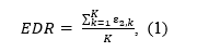
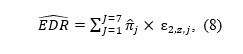
The EDR,
is defined as the mean power (ε2) of a set of K studies, independent on the outcome direction.
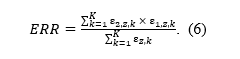
Following Brunner and Schimmack (2020), the expected replication rate (ERR) is defined as the ratio of mean squared power and mean power of all studies, statistically significant and non-significant ones. We modify the definition here by taking the direction of the replication study into account.[2] The mean square power in the nominator is used because we are computing the expected relative frequency of statistically significant studies produced by a set of already statistically significant studies – if a study produces a statistically significant result with probability equal to its power, the chance that the same study will again be significant is power squared. The mean power in the denominator is used because we are restricting our selection to only already statistically significant studies which are produced at the rate corresponding to their power (see also Miller, 2009). The ratio simplifies by omitting division by K in both the nominator and denominator to:
which can also be read as a weighted mean power, where each power is weighted by itself. The weights originate from the fact that studies with higher power are more likely to produce statistically significant results. The weighted mean power of all studies is therefore equal to the unweighted mean power of the studies selected for significance (ksig; cf. Brunner & Schimmack, 2020).
If we have a set of studies with the same power (e.g., set of exact replications with the same sample size) that test for an effect with a z-test, the p-values converted to z-statistics follow a normal distribution with mean and a standard deviation equal to 1. Using an alpha level α, the power is the tail area of a standard normal distribution (Φ) centered over a mean, (μz) on the left and right side of the z-scores corresponding to alpha, -1.96 and 1.96 (with the usual alpha = .05),
or the tail area on the right side of the z-score corresponding to alpha, when we are also considering whether the directionality of the effect,
Two-sided p-values do not preserve the direction of the deviation from null and we cannot know whether a z-statistic comes from the lower or upper tail of the distribution. Therefore, we work with absolute values of z-statistics, changing their distribution from normal to folded normal distribution (Elandt, 1961; Leone, Nelson, & Nottingham, 1961).
Figure 1 illustrates the key concepts of z-curve with various examples. The first three density plots in the first row show the sampling distributions for studies with low (ε = 0.3), medium (ε = 0.5), and high (ε = .8) power, respectively. The last density plots illustrate the distribution that is obtained for a mixture of studies with low, medium, and high power with equal frequency (33.3% each). It is noteworthy that all four density distributions have different shapes. While Figure 1 illustrates how differences in power produce differences in the shape of the distributions, z-curve works backward and uses the shape of the distribution to estimate power.
Figure 1. Density (y-axis) of z-statistics (x-axis) generated by studies with different powers (columns) across different stages of the publication process (rows). The first row shows a distribution of z-statistics from z-tests homogeneous in power (the first three columns) or by their mixture (the fourth column). The second row shows only statistically significant z-statistics. The third row visualizes EDR as a proportion of statistically significant z-statistics out of all z-statistics. The fourth row shows a distribution of z-statistics from exact replications of only the statistically significant studies (dashed line for non-significant replication studies). The fifth row visualizes ERR as a proportion of statistically significant exact replications out of statistically significant studies.
Although z-curve can be used to fit the distributions in the first row, we assume that the observed distribution of all z-statistics is distorted by the selection bias. Even if some statistically non-significant p-values are reported, their distribution is subject to unknown selection effects. Therefore, by default z-curve assumes that selection bias is present and uses only the distribution of statistically significant results. This changes the distributions of z-statistics to folded normal distributions that are truncated at the z-score corresponding to the significance criterion, which is typically z = 1.96 for p = .05 (two-tailed). The second row in Figure 1 shows these truncated folded normal distributions. Importantly, studies with different levels of power produce different distributions despite the truncation. The different shapes of truncated distributions make it possible to estimate power by fitting a model to the truncated distribution. The third row of Figure 1 illustrates the EDR as a proportion of statistically significant studies from all conducted studies. We use Equation 3 to re-express EDR (Equation 2), which equals the mean unconditional power, of a set of K heterogenous studies using the means of sampling distributions of their z-statistics, μz,k,
Z-curve makes it possible to estimate the shape of the distribution in the region of statistically non-significant results on the basis of the observed distribution of statistically significant results. That is, after fitting a model to the grey area of the curve, it extrapolates the full distribution.
The fourth row of Figure 1 visualizes a distribution of expected z-statistics if the statistically significant studies were to be exactly replicated (not depicting the small proportion of results in the opposite direction than the original, significant, result). The full line highlights the portion of studies that would produce a statistically significant result, with the distribution of statistically non-significant studies drawn using the dashed line. An exact replication with the same sample size of the studies in the grey area in the second row is not expected to reproduce the truncated distribution again because truncation is a selection process. The replication distribution is not truncated and produces statistically significant and non-significant results. By modeling the selection process, z-curve predicts the non-truncated distributions in the fourth row from the truncated distributions in the second row.
The fifth row of Figure 1 visualizes ERR as a proportion of statistically significant exact replications in the expected direction from a set of the previously statistically significant studies. The ERR (Equation 1) of a set ofheterogeneous studies can be again re-expressed using Equations 3 and 4 with the means of sampling distributions of their z-statistics,
Z-curve 2.0
Z-curve is a finite mixture model (Brunner & Schimmack, 2020). Finite mixture models leverage the fact that an observed distribution of statistically significant z-statistics is a mixture of K truncated folded normal distribution with means and standard deviations 1. Instead of trying to estimate of every single observed z-statistic, a finite mixture model approximates the observed distribution based on K studies with a smaller set of J truncated folded normal distributions, , with J < K components,
Each mixture component j approximates a proportion of observed z-statistics with a probability density function, , of truncated folded normal distribution with parameters – a mean and standard deviation equal to 1. For example, while actual studies may vary in power from 40% to 60%, a mixture model may represent all of these studies with a single component with 50% power.
Z-curve 1.0 used three components with varying means. Extensive testing showed that varying means produced poor estimates of the EDR. Therefore, we switched to models with fixed means and increased the number of components to seven. The seven components are equally spaced by one standard deviation from z = 0 (power = alpha) to 6 (power ~ 1). As power for z-scores greater than 6 is essentially 1, it is not necessary to model the distribution of z-scores greater than 6, and all z-scores greater than 6 are assigned a power value of 1 (Brunner & Schimmack, 2020). The power values implied by the 7 components are .05, .17, .50, .85, .98, .999, .99997. We also tried a model with equal spacing of power, and we tried models with fewer or more components, but neither did improve performance in simulation studies.
We use the model parameter estimates to compute the estimated the EDR and ERR as the weighted average of seven truncated folded normal distributions centered over z = 0 to 6,
Curve Fitting
Z-curve 1.0 used an unorthodox approach to find the best fitting model that required fitting a truncated kernel-density distribution to the statistically significant z-statistics (Brunner & Schimmack, 2020). This is a non-trivial step that may produce some systematic bias in estimates. Z-curve 2.0 makes it possible to fit the model directly to the observed z-statistics using the well-established expectation maximization (EM) algorithm that is commonly used to fit mixture models (Dempster, Laird, & Rubin, 1977, Lee & Scott, 2012). Using the EM algorithm has the advantage that it is a well-validated method to fit mixture models. It is beyond the scope of this article to explain the mechanics of the EM algorithm (cf. Bishop, 2006), but it is important to point out some of its potential limitations. The main limitation is that it may terminate the search for the best fit before the best fitting model has been found. In order to prevent this, we run 20 searches with randomly selected starting values and terminate the algorithm in the first 100 iterations, or if the criterion falls below 1e-3. We then select the outcome with the highest likelihood value and continue until 1000 iterations or a criterion value of 1e-5 is reached. To speed up the fitting process, we optimized the procedure using Rcpp (Eddelbuettel et al., 2011).
Information about point estimates should be accompanied by information about uncertainty whenever possible. The most common way to do so is by providing confidence intervals. We followed the common practice of using bootstrapping to obtain confidence intervals for mixture models (Ujeh et al., 2016). As bootstrapping is a resource-intensive process, we used 500 samples for the simulation studies. Users of the z-curve package can use more iterations to analyze actual data.
Simulations
Brunner and Schimmack (2020) compared several methods for estimating mean power and found that z-curve performed better than three competing methods. However, these simulations were limited to the estimation of the ERR. Here we present new simulation studies to examine the performance of z-curve as a method to estimate the EDR as well. One simulation directly simulated power distributions, the other one simulated t-tests. We report the detailed results of both simulation studies in a Supplement. For the sake of brevity, we focus on the simulation of t-tests because readers can more easily evaluate the realism of these simulations. Moreover, most tests in psychology are t-tests or F-tests and Bruner and Schimmack (2020) already showed that the numerator degrees of freedom of F-tests do not influence results. Thus, the results for t-tests can be generalized to F-tests and z-tests.
The simulation was a complex 4 x 4 x 4 x 3 x 3 design with 576 cells. The first factor of the design that was manipulated was the mean effect size with Cohen’s ds ranging from 0 to 0.6 (0, 0.2, 0.4., 0.6). The second factor in the design was heterogeneity in effect sizes was simulated with a normal distribution around the mean effect size with SDs ranging from 0 to 0.6 (0, 0.2, 0.4., 0.6). Preliminary analysis with skewed distributions showed no influence of skew. The third factor of the design was sample size for between-subject design with N = 50, 100, and 200. The fourth factor of the design was the percentage of true null-hypotheses that ranged from 0 to 60% (0%, 20%, 40%, 60%). The last factor of the design was the number of studies with sets of k = 100, 300, and 1,000 statistically significant studies.
Each cell of the design was run 100 times for a total of 57,600 simulations. For the main effects of this design there were 57,600 / 4 = 14,400 or 57,600 / 3 = 19,200 simulations. Even for two-way interaction effects, the number of simulations is sufficient, 57,600 / 16 = 3,600. For higher interactions the design may be underpowered to detect smaller effects. Thus, our simulation study meets recommendations for sample sizes in simulation studies for main effects and two-way interactions, but not for more complex interaction effects (Morris, White, & Crowther, 2019). The code for the simulations is accessible at https://osf.io/r6ewt/.
Evaluation
For a comprehensive evaluation of z-curve 2.0 estimates, we report bias (i.e., mean distance between estimated and true values), root mean square error (RMSE; quantifying the error variance of the estimator), and confidence interval coverage (Morris et al. 2019).[3] To check the performance of the z-curve across different simulation settings, we analyzed the results of the factorial design using analyses of variance (ANOVAs) for continuous measures and logistic regression for the evaluation of confidence intervals (0 = true value not in the interval, 1 = true value in the interval). The analysis scripts and results are accessible at https://osf.io/r6ewt/.
Results
We start with the ERR because it is essentially a conceptual replication study of Brunner and Schimmack’s (2020) simulation studies with z-curve 1.0.
ERR
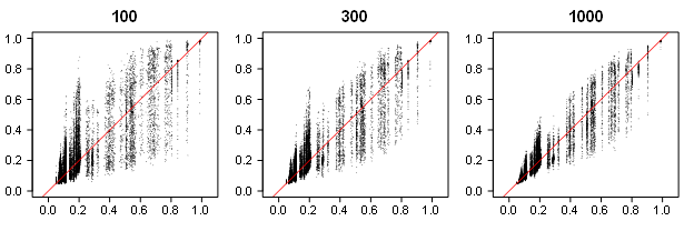
Visual inspection of the z-curves ERR estimates plotted against the true ERR values did not show any pathological behavior due to the approximation by a finite mixture model (Figure 3).
Figure 3. Estimated (y-axis) vs. true (x-axis) ERR in simulation U across a different number of studies.
Figure 3 shows that even with k = 100 studies, z-curve estimates are clustered close enough to the true values to provide useful predictions about the replicability of sets of studies. Overall bias was less than one percentage point, -0.88 (SEMCMC = 0.04). This confirms that z-curve has high large-sample accuracy (Brunner & Schimmack, 2020). RMSE decreased from 5.14 (SEMCMC = 0.03) percentage points with k = 100 to 2.21 (SEMCMC = 0.01) percentage points with k = 1,000. Thus, even with relatively small sample sizes of 100 studies, z-curve can provide useful information about the ERR.
The Analysis of Variance (ANOVA) showed no statistically significant 5-way interaction or 4-way interactions. A strong three-way interaction was found for effect size, heterogeneity of effect sizes, and sample size, z = 9.42. Despite the high statistical significance, effect sizes were small. Out of the 36 cells of the 4 x 3 x 3 design, 32 cells showed less than one percentage point bias. Larger biases were found when effect sizes were large, heterogeneity was low, and sample sizes were small. The largest bias was found for Cohen’s d = 0.6, SD = 0, and N = 50. In this condition, ERR was 4.41 (SEMCMC = 0.11) percentage points lower than the true replication rate. The finding that z-curve performs worse with low heterogeneity replicates findings by Brunner and Schimmack (2002). One reason could be that a model with seven components can easily be biased when most parameters are zero. The fixed components may also create a problem when true power is between two fixed levels. Although a bias of 4 percentage points is not ideal, it also does not undermine the value of a model that has very little bias across a wide range of scenarios.
The number of studies had a two-way interaction with effect size, z = 3.8, but bias in the 12 cells of the 4 x 3 design was always less than 2 percentage points. Overall, these results confirm the fairly good large sample accuracy of the ERR estimates.
We used logistic regression to examine patterns in the coverage of the 95% confidence intervals. This time a statistically significant four-way interaction emerged for effect size, heterogeneity of effect sizes, sample size, and the percentage of true null-hypotheses, z = 10.94. Problems mirrored the results for bias. Coverage was low when there were no true null-hypotheses, no heterogeneity in effect sizes, large effects, and small sample sizes. Coverage was only 31.3% (SEMCMC = 2.68) when the percentage of true H0 was 0, heterogeneity of effect sizes was 0, the effect size was Cohen’s d = 0.6, and the sample size was N = 50.
In statistics, it is common to replace confidence intervals that fail to show adequate coverage with confidence intervals that provide good coverage with real data; these confidence intervals are often called robust confidence intervals (Royall, 1996). We suspected that low coverage was related to systematic bias. When confidence intervals are drawn around systematically biased estimates, they are likely to miss the true effect size by the amount of systematic bias, when sampling error pushes estimates in the same direction as the systematic bias. To increase coverage, it is therefore necessary to take systematic bias into account. We created robust confidence intervals by adding three percentage points on each side. This is very conservative because the bias analysis would suggest that only adjustment in one direction is needed.
The logistic regression analysis still showed some statistically significant variation in coverage. The most notable finding was a 2-way interaction for effect size and sample size, z = 4.68. However, coverage was at 95% or higher for all 12 cells of the design. Further inspection showed that the main problem remained scenarios with high effect sizes (d = 0.6) and no heterogeneity (SD = 0), but even with small heterogeneity, SD = 0.2, this problem disappeared. We therefore recommend extending confidence intervals by three percentage points. This is the default setting in the z-curve package, but the package allows researchers to change these settings. Moreover, in meta-analyses of studies with low heterogeneity, alternative methods that are more appropriate for homogeneous methods (e.g., selection models; Hedges, 1992) may be used or the number of components could be reduced.
EDR
Visual inspection of EDRs plotted against the true discovery rates (Figure 4) showed a noticeable increase in uncertainty. This is to be expected as EDR estimates require estimation of the distribution for statistically non-significant z-statistics solely on the basis of the distribution of statistically significant results.
Figure 4. Estimated (y-axis) vs. true (x-axis) EDR across a different number of studies.
Despite the high variability in estimates, they can be useful. With the observed discovery rate in psychology being often over 90% (Sterling, 1959), many of these estimates would alert readers that selection bias is present. A bigger problem is that the highly variable EDR estimates might lack the power to detect selection bias in small sets of studies.
Across all studies, systematic bias was small, 1.42 (SEMCMC = 0.08) for 100 studies, 0.57 (SEMCMC = 0.06) for 300 studies, 0.16 (SEMCMC = 0.05) percentage points for 1000 studies. This shows that the shape of the distribution of statistically significant results does provide valid information about the shape of the full distribution. Consistent with Figure 4, RMSE values were large and remained fairly large even with larger number of studies, 11.70 (SEMCMC = 0.11) for 100 studies, 8.88 (SEMCMC = 0.08) for 300 studies, 6.49 (SEMCMC = 0.07) percentage points for 1000 studies. These results show how costly selection bias is because more precise estimates of the discovery rate would be available without selection bias.
The main consequence of high RMSE is that confidence intervals are expected to be wide. The next analysis examined whether confidence intervals have adequate coverage. This was not the case; coverage = 87.3% (SEMCMC = 0.14). We next used logistic regression to examine patterns in coverage in our simulation design. A notable 3-way interaction between effect size, sample size, and percentage of true H0 was present, z = 3.83. While the pattern was complex, not a single cell of the design showed coverage over 95%.
As before, we created robust confidence intervals by extending the interval. We settled for an extension by five percentage points. The 3-way interaction remained statistically significant, z = 3.36. Now 43 of the 48 cells showed coverage over 95%. For reasons that are not clear to us, the main problem occurred for an effect size of Cohen’s d = 0.4 and no true H0, independent of sample size. While improving the performance of z-curve remains an important goal and future research might find better approaches to address this problem, for now, we recommend using z-curve 2.0 with these robust confidence intervals, but users can specify more conservative adjustments.
Application to Real Data
It is not easy to evaluate the performance of z-curve 2.0 estimates with actual data because selection bias is ubiquitous and direct replication studies are fairly rare (Zwaan, Etz, Lucas, & Donnellan, 2018). A notable exception is the Open Science Collaboration project that replicated 100 studies from three psychology journals (Open Science Collaboration, 2015). This unprecedented effort has attracted attention within and outside of psychological science and the article has already been cited over 1,000 times. The key finding was that out of 97 statistically significant results, including marginally significant ones, only 36 replication studies (37%) reproduced a statistically significant result in the replication attempts.
This finding has produced a wide range of reactions. Often the results are cited as evidence for a replication crisis in psychological science, especially social psychology (Schimmack, 2020). Others argue that the replication studies were poorly carried out and that many of the original results are robust findings (Bressan, 2019). This debate mirrors other disputes about failures to replicate original results. The interpretation of replication studies is often strongly influenced by researchers’ a priori beliefs. Thus, they rarely settle academic disputes. Z-curve analysis can provide valuable information to determine whether an original or a replication study is more trustworthy. If a z-curve analysis shows no evidence for selection bias and a high ERR, it is likely that the original result is credible and the replication failure is a false negative result or the replication study failed to reproduce the original experiment. On the other hand, if there is evidence for selection bias and the ERR is low, replication failures are expected because the original results were obtained with questionable research practices.
Another advantage of z-curve analyses of published results is that it is easier to obtain large representative samples of studies than to conduct actual replication studies. To illustrate the usefulness of z-curve analyses, we focus on social psychology because this field has received the most attention from meta-psychologists (Schimmack, 2020). We fitted z-curve 2.0 to two studies of published test statistics from social psychology and compared these results to the actual success rate in the Open Science Collaboration project (k = 55).
One sample is based on Motyl et al.’s (2017) assessment of the replicability of social psychology (k = 678). The other sample is based on the coding of the most highly cited articles by social psychologists with a high H-Index (k = 2,208; Schimmack, 2021). The ERR estimates were 44%, 95% CI [35, 52]%, and 51%, 95% CI [45, 56]%. The two estimates do not differ significantly from each other, but both estimates are considerably higher than the actual discovery rate in the OSC replication project, 25%, 95% CI [13, 37]%. We postpone the discussion of this discrepancy to the discussion section.
The EDRs estimates were 16%, 95% CI [5, 32]%, and 14%, 95% CI [7, 23]%. Again, both of the estimates overlap and do not significantly differ. At the same time, the EDR estimates are much lower than the ODRs in these two data sets (90%, 89%). The z-curve analysis of published results in social psychology shows a strong selection bias that explains replication failures in actual replication attempts. Thus, the z-curve analysis reveals that replication failures cannot be attributed to problems of the replication attempts. Instead, the low EDR estimates show that many non-significant original results are missing from the published record.
Discussion
A previous article introduced z-curve as a viable method to estimate mean power after selection for significance (Brunner & Schimmack, 2020). This is a useful statistic because it predicts the success rate of exact replication studies. We therefore call this statistic the expected replication rate. Studies with a high replication rate provide credible evidence for a phenomenon. In contrast, studies with a low replication rate are untrustworthy and require additional evidence.
We extended z-curve 1.0 in two ways. First, we implemented the expectation maximization algorithm to fit the mixture model to the observed distribution of z-statistics. This is a more conventional method to fit mixture models. We found that this method produces good estimates, but it did not eliminate some of the systematic biases that were observed with z-curve 1.0. More important, we extended z-curve to estimate the mean power before selection for significance. We call this statistic the expected discovery rate because mean power predicts the percentage of statistically significant results for a set of studies. We found that EDR estimates have satisfactory large sample accuracy, but vary widely in smaller sets of studies. This limits the usefulness for meta-analysis of small sets of studies, but as we demonstrated with actual data, the results are useful when a large set of studies is available. The comparison of the EDR and ODR can also be used to assess the amount of selection bias. A low EDR can also help researchers to realize that they test too many false hypotheses or test true hypotheses with insufficient power.
In contrast to Miller (2009), who stipulates that estimating the ERR (“aggregated replication probability”) is unattainable due to selection processes, Schimmack and Brunner’s (2020) z-curve 1.0 addresses the issue by modeling the selection for significance.
Finally, we examined the performance of bootstrapped confidence intervals in simulation studies. We found that coverage for 95% confidence intervals was sometimes below 95%. To improve the coverage of confidence intervals, we created robust confidence intervals that added three percentage points to the confidence interval of the ERR and five percentage points to the confidence interval of the EDR.
We demonstrate the usefulness of the EDR and confidence intervals with an example from social psychology. We find that ERR overestimates the actual replicability in social psychology. We also find clear evidence that power in social psychology is low and that high success rates are mostly due to selection for significance. It is noteworthy that while the Motyl et al.’s (2017) dataset is representative for social psychology, Schimmack’s (2021) dataset sampled highly influential articles. The fact that both sampling procedures produced similar results suggests that studies by eminent researchers or studies with high citation rates are no more replicable than other studies published in social psychology.
Z-curve 2.0 does provide additional valuable information that was not provided by z-curve 1.0. Moreover, z-curve 2.0 is available as an R-package, making it easier for researchers to conduct z-curve analyses (Bartoš & Schimmack, 2020). This article provides the theoretical background for the use of the z-curve package. Subsequently, we discuss some potential limitations of z-curve 2.0 analysis and compare z-curve 2.0 to other methods that aim to estimate selection bias or power of studies.
Bias Detection Methods
In theory, bias detection is as old as meta-analysis. The first bias test showed that Mendel’s genetic experiments with peas had less sampling error than a statistical model would predict (Pires & Branco, 2010). However, when meta-analysis emerged as a widely used tool to integrate research findings, selection bias was often ignored. Psychologists focused on fail-safe N (Rosenthal, 1979), which did not test for the presence of bias and often led to false conclusions about the credibility of a result (Ferguson & Heene, 2012). The most common tools to detect bias rely on correlations between effect sizes and sample size. A key problem with this approach is that it often has low power and that results are not trustworthy under conditions of heterogeneity (Inzlicht, Gervais, & Berkman, 2015; Renkewitz & Keiner, 2019). The tests are also not useful for meta-analysis of heterogeneous sets of studies where researchers use larger samples to study smaller effects, which also introduces a correlation between effect sizes and sample sizes. Due to these limitations, evidence of bias has been dismissed as inconclusive (Cunningham & Baumeister, 2016; Inzlicht & Friese; 2019).
It is harder to dismiss evidence of bias when a set of published studies has more statistically significant results than the power of the studies warrants; that is, the ODR exceeds the EDR (Sterling et al., 1995). Aside from z-curve 2.0, there are two other bias tests that rely on a comparison of the ODR and EDR to evaluate the presence of selection bias, namely the Test of Excessive Significance (TES, Ioannidis & Trikalinos, 2005) and the Incredibility Test (IT; Schimmack, 2012).
Z-curve 2.0 has several advantages over the existing methods. First, TES was explicitly designed for meta-analysis with little heterogeneity and may produce biased results when heterogeneity is present (Renkewitz & Keiner, 2019). Second, both the TES and the IT take observed power at face value. As observed power is inflated by selection for significance, the tests have low power to detect selection for significance, unless the selection bias is large. Finally, TES and IT rely on p-values to provide information about bias. As a result, they do not provide information about the amount of selection bias.
Z-curve 2.0 overcomes these problems by correcting the power estimate for selection bias, providing quantitative evidence about the amount of bias by comparing the ODR and EDR, and by providing evidence about statistical significance by means of a confidence interval around the EDR estimate. Thus, z-curve 2.0 is a valuable tool for meta-analysts, especially when analyzing a large sample of heterogenous studies that vary widely in designs and effect sizes. As we demonstrated with our example, the EDR of social psychology studies is very low. This information is useful because it alerts readers to the fact that not all p-values below .05 reveal a true and replicable finding.
Nevertheless, z-curve has some limitations. One limitation is that it does not distinguish between significant results with opposite signs. In the presence of multiple tests of the same hypothesis with opposite signs, researchers can exclude inconsistent significant results and estimate z-curve on the basis of significant results with the correct sign. However, the selection of tests by the meta-analyst introduces additional selection bias, which has to be taken into account in the comparison of the EDR and ODR. Another limitation is the assumption that all studies used the same alpha criterion (.05) to select for significance. This possibility can be explored by conducting multiple z-curve analyses with different selection criteria (e.g., .05, .01). The use of lower selection criteria is also useful because some questionable research practices produce a cluster of just significant results. However, all statistical methods can only produce estimates that come with some uncertainty. When severe selection bias is present, new studies are needed to provide credible evidence for a phenomenon.
Predicting Replication Outcomes
Since 2011, many psychologists have learned that published significant results can have a low replication probability (Open Science Collaboration, 2015). This makes it difficult to trust the published literature, especially older articles that report results from studies with small samples that were not pre-registered. Should these results be disregarded because they might have been obtained with questionable research practices? Should results only be trusted if they have been replicated in a new, ideally pre-registered, replication study? Or should we simply assume that most published results are probably true and continue to treat every p-value below .05 as a true discovery?
The appeal of z-curve is that we can use the published evidence to distinguish between credible and “incredible” (biased) statistically significant results. If a meta-analysis shows low selection bias and a high replication rate, the results are credible. If a meta-analysis shows high selection bias and a low replication rate, the results are incredible and require independent verification.
As appealing as this sounds, every method needs to be validated before it can be applied to answer substantive questions. This is also true for z-curve 2.0. We used the results from the OSC replicability project for this purpose. The results suggest that z-curve predictions of replication rates may be overly optimistic. While the expected replication rate was between 44% and 51% (35% – 56% CI range), the actual success rate was only 25%, 95% CI [13, 37]%. Thus, it is important to examine why z-curve estimates are higher than the actual replication rate in the OSC project.
One possible explanation is that there is a problem with the replication studies. Social psychologists quickly criticized the quality of the replication studies (Gilbert, King, Pettigrew, & Wilson, 2016). In response, the replication team conducted the new replications of contested replication studies. Based on the effect sizes in these much larger replication studies, not a single original study would have produced statistically significant results (Ebersole et al., 2020). It is therefore unlikely that the quality of replication studies explains the low success rate of replication studies in social psychology.
A more interesting explanation is that social psychological phenomena are not as stable as boiling distilled water under tightly controlled laboratory conditions. Rather, effect sizes vary across populations, experimenters, times of day, and a myriad of other factors that are difficult to control (Stroebe & Strack, 2014). In this case, selection for significance produces additional regression to the mean because statistically significant results were obtained with the help of favorable hidden moderators that produced larger effect sizes that are unlikely to be present again in a direct replication study.
The worst-case scenario is that studies that were selected for significance are no more powerful than studies that produced statistically non-significant results. In this case, the EDR predicts the outcome of actual replication studies. Consistent with this explanation, the actual replication rate of 25%, 95% CI [13, 37]%, was highly consistent with the EDR estimates of 16%, 95% CI [5, 32]%, and 14%, 95% CI [7, 23]%. More research is needed once more replication studies become available to see how closely actual replication rates are to the EDR and the ERR. For now, they should be considered the worst and the best possible scenarios and actual replication rates are expected to fall somewhere between these two estimates.
A third possibility for the discrepancy is that questionable research practices change the shape of the z-curve in ways that are different from a simple selection model. For example, if researchers have several statistically significant results and pick the highest one, the selection model underestimates the amount of selection that occurred. This can bias z-curve estimates and inflate the ERR and EDR estimates. Unfortunately, it is also possible that questionable research practices have the opposite effect and that ERR and EDR estimates underestimate the true values. This uncertainty does not undermine the usefulness of z-curve analyses. Rather it shows how questionable research practices undermine the credibility of published results. Z-curve 2.0 does not alleviate the need to reform research practices and to ensure that all researchers report their results honestly.
Conclusion
Z-curve 1.0 made it possible to estimate the replication rate of a set of studies on the basis of published test results. Z-curve 2.0 makes it possible to also estimate the expected discovery rate; that is, how many tests were conducted to produce the statistically significant results. The EDR can be used to evaluate the presence and amount of selection bias. Although there are many methods that have the same purpose, z-curve 2.0 has several advantages over these methods. Most importantly, it quantifies the amount of selection bias. This information is particularly useful when meta-analyses report effect sizes based on methods that do not consider the presence of selection bias.
Author Contributions
Most of the ideas in the manuscript were developed jointly. The main idea behind the z-curve method and its density version was developed by Dr. Schimmack. Mr. Bartoš implemented the EM version of the method and conducted the extensive simulation studies.
Acknowledgments
Access to computing and storage facilities owned by parties and projects contributing to the National Grid Infrastructure MetaCentrum provided under the program “Projects of Large Research, Development, and Innovations Infrastructures” (CESNET LM2015042), is greatly appreciated. We would like to thank Maximilian Maier, Erik W. van Zwet, and Leonardo Tozzi for valuable comments on a draft of this manuscript.
No conflict of interest to report. This work was not supported by a specific grant.
References
Bartoš, F., & Maier, M. (in press). Power or alpha? The better way of decreasing the false discovery rate. Meta-Psychology. https://doi.org/10.31234/osf.io/ev29a
Bartoš, F., & Schimmack, U. (2020). “zcurve: An R Package for Fitting Z-curves.” R package version 1.0.0
Begley, C. G., & Ellis, L. M. (2012). Raise standards for preclinical cancer research. Nature, 483(7391), 531–533. https://doi.org/10.1038/483531a
Bishop, C. M. (2006). Pattern recognition and machine learning. Springer.
Boos, D. D., & Stefanski, L. A. (2011). P-value precision and reproducibility. The American Statistician, 65(4), 213-221. https://doi.org/10.1198/tas.2011.10129
Brunner, J. & Schimmack, U. (2020). Estimating population mean power under conditions of heterogeneity and selection for significance. Meta-Psychology, 4, https://doi.org/10.15626/MP.2018.874
Camerer, C. F., Dreber, A., Forsell, E., Ho, T. H., Huber, J., Johannesson, M., … & Heikensten, E. (2016). Evaluating replicability of laboratory experiments in economics. Science, 351(6280). https://doi.org/10.1126/science.aaf0918
Chang, Andrew C., and Phillip Li (2015). Is economics research replicable? Sixty published papers from thirteen journals say ”usually not”, Finance and Economics Discussion Series 2015-083. Washington: Board of Governors of the Federal Reserve System. http://dx.doi.org/10.17016/FEDS.2015.083.
Chase, L. J., & Chase, R. B. (1976). Statistical power analysis of applied psychological research. Journal of Applied Psychology, 61(2), 234–237. https://doi.org/10.1037/0021-9010.61.2.234
Cunningham, M. R., & Baumeister, R. F. (2016). How to make nothing out of something: Analyses of the impact of study sampling and statistical interpretation in misleading meta-analytic conclusions. Frontiers in Psychology, 7, 1639. https://doi.org/10.3389/fpsyg.2016.01639
Dempster, A. P., Laird, N. M., & Rubin, D. B. (1977). Maximum likelihood from incomplete data via the EM algorithm. Journal of the Royal Statistical Society: Series B (Methodological), 39(1), 1–22. https://doi.org/10.1111/j.2517-6161.1977.tb01600.x
Ebersole, C. R., Mathur, M. B., Baranski, E., Bart-Plange, D.-J., Buttrick, N. R., Chartier, C. R., Corker, K. S., Corley, M., Hartshorne, J. K., IJzerman, H., Lazarević, L. B., Rabagliati, H., Ropovik, I., Aczel, B., Aeschbach, L. F., Andrighetto, L., Arnal, J. D., Arrow, H., Babincak, P., … Nosek, B. A. (2020). Many Labs 5: Testing pre-data-collection peer review as an intervention to increase replicability. Advances in Methods and Practices in Psychological Science, 3(3), 309–331. https://doi.org/10.1177/2515245920958687
Egger, M., Smith, G. D., Schneider, M., & Minder, C. (1997). Bias in meta-analysis detected by a simple, graphical test. BMJ,315(7109), 629-634. https://doi.org/10.1136/bmj.315.7109.629
Eddelbuettel, D., François, R., Allaire, J., Ushey, K., Kou, Q., Russel, N., … Bates, D. (2011). Rcpp: Seamless R and C++ integration. Journal of Statistical Software, 40(8), 1–18. https://doi.org/10.18637/jss.v040.i08
Elandt, R. C. (1961). The folded normal distribution: Two methods of estimating parameters from moments. Technometrics, 3(4), 551–562. https://doi.org/10.2307/1266561
Ferguson, C. J., & Heene, M. (2012). A vast graveyard of undead theories: Publication bias and psychological science’s aversion to the null. Perspectives on Psychological Science, 7(6), 555–561. https://doi.org/10.1177/1745691612459059
Francis G., (2014). The frequency of excess success for articles in Psychological Science. Psychonomic Bulletin and Review, 21, 1180–1187. https://doi.org/10.3758/s13423-014-0601-x
Franco, A., Malhotra, N., & Simonovits, G. (2014). Publication bias in the social sciences: Unlocking the file drawer. Science, 345(6203), 1502-1505. . https://doi.org/10.1126/science.1255484
Gilbert, D. T., King, G., Pettigrew, S., & Wilson, T. D. (2016). Comment on “Estimating the reproducibility of psychological science.” Science,351, 1037–1103. http://dx.doi.org/10.1126/science.aad7243
Hedges, L. V. (1992). Modeling publication selection effects in meta-analysis. Statistical Science,7(2), 246–255. https://doi.org/10.1214/ss/1177011364
Inzlicht, M., Gervais, W., & Berkman, E. (2015). Bias-correction techniques alone cannot determine whether ego depletion is different from zero: Commentary on Carter, Kofler, Forster, & McCullough, 2015. Kofler, Forster, & McCullough. http://dx.doi.org/10.2139/ssrn.2659409
Ioannidis, J. P., & Trikalinos, T. A. (2007). An exploratory test for an excess of significant findings. Clinical Trials, 4(3), 245–253. https://doi.org/10.1177/1740774507079441
John, L. K., Lowenstein, G., & Prelec, D. (2012). Measuring the prevalence of questionable research practices with incentives for truth telling. Psychological Science, 23, 517–523. https://doi.org/10.1177/0956797611430953
Lee, G., & Scott, C. (2012). EM algorithms for multivariate Gaussian mixture models with truncated and censored data. Computational Statistics & Data Analysis, 56(9), 2816–2829. https://doi.org/10.1016/j.csda.2012.03.003
Maier, M., Bartoš, F., & Wagenmakers, E. (in press). Robust Bayesian meta-analysis: Addressing publication bias with model-averaging. Psychological Methods. https://doi.org/10.31234/osf.io/u4cns
Miller, J. (2009). What is the probability of replicating a statistically significant effect?. Psychonomic Bulletin & Review 16, 617–640. https://doi.org/10.3758/PBR.16.4.617
Morris, T. P., White, I. R., & Crowther, M. J. (2019). Using simulation studies to evaluate statistical methods. Statistics in Medicine, 38(11), 2074-2102. https://doi.org/10.1002/sim.8086
Motyl, M., Demos, A. P., Carsel, T. S., Hanson, B. E., Melton, Z. J., Mueller, A. B., Prims, J. P., Sun, J., Washburn, A. N., Wong, K. M., Yantis, C., & Skitka, L. J. (2017). The state of social and personality science: Rotten to the core, not so bad, getting better, or getting worse? Journal of Personality and Social Psychology, 113(1), 34–58. https://doi.org/10.1037/pspa0000084
Open Science Collaboration. (2015). Estimating the reproducibility of psychological science. Science, 349(6251), aac4716–aac4716. https://doi.org/10.1126/science.aac4716
Pashler, H., & Wagenmakers, E. J. (2012). Editors’ introduction to the special section on replicability in psychological science: A crisis of confidence? Perspectives on Psychological Science, 7(6), 528-530. https://doi.org/10.1177/1745691612465253
Pires, A. M., & Branco, J. A. (2010). A statistical model to explain the Mendel—Fisher controversy. Statistical Science, 545-565. https://doi.org/10.1214/10-STS342
Prinz, F., Schlange, T., & Asadullah, K. (2011). Believe it or not: how much can we rely on published data on potential drug targets? Nature Reviews Drug Discovery, 10(9), 712–712. https://doi.org/10.1038/nrd3439-c1
Renkewitz, F., & Keiner, M. (2019). How to detect publication bias in psychological research. Zeitschrift für Psychologie. https://doi.org/10.1027/2151-2604/a000386
Rosenthal, R., & Gaito, J. (1964). Further evidence for the cliff effect in interpretation of levels of significance. Psychological Reports 15(2), 570.https://doi.org/10.2466/pr0.1964.15.2.570
Scheel, A. M., Schijen, M. R., & Lakens, D. (2021). An excess of positive results: Comparing the standard Psychology literature with Registered Reports. Advances in Methods and Practices in Psychological Science, 4(2), https://doi.org/10.1177/25152459211007467
Schimmack, U. (2012). The ironic effect of significant results on the credibility of multiple-study articles. Psychological Methods, 17, 551–566. https://doi.org/10.1037/a0029487
Schimmack, U. (2020). A meta-psychological perspective on the decade of replication failures in social psychology. Canadian Psychology/Psychologie canadienne. 61 (4), 364-376. https://doi.org/10.1037/cap0000246
Sorić, B. (1989). Statistical “discoveries” and effect-size estimation. Journal of the American Statistical Association, 84(406), 608-610. https://doi.org/10.2307/2289950
Sterling, T. D. (1959). Publication decision and the possible effects on inferences drawn from tests of significance – or vice versa. Journal of the American Statistical Association, 54, 30–34. https://doi.org/10.2307/2282137
Sterling, T. D., Rosenbaum, W. L., & Weinkam, J. J. (1995). Publication decisions revisited: The effect of the outcome of statistical tests on the decision to publish and vice versa. The American Statistician, 49, 108–112. https://doi.org/10.2307/2684823
Stroebe, W., & Strack, F. (2014). The alleged crisis and the illusion of exact replication. Perspectives on Psychological Science, 9, 59–71. http://dx.doi.org/10.1177/1745691613514450
Vevea, J. L., & Hedges, L. V. (1995). A general linear model for estimating effect size in the presence of publication bias. Psychometrika, 60(3), 419–435. https://doi.org/10.1007/BF02294384
Wegner, D. M. (1992). The premature demise of the solo experiment. Personality and Social Psychology Bulletin, 18(4), 504-508. https://doi.org/10.1177/0146167292184017
Zwaan, R. A., Etz, A., Lucas, R. E., & Donnellan, M. B. (2018). Making replication mainstream. Behavioral and Brain Sciences, 41, Article e120. https://doi.org/10.1017/S0140525X17001972
Footnotes
[1] In reality, sampling erorr will produce an observed discovery rate that deviates slightly from the expected discovery rate. To keep things simple, we assume that the observed discovery rate matches the expected discovery rate perfectly.
[2] We thank Erik van Zwet for suggesting this modification in his review and for many other helpful comments.
[3] To compute MCMC standard errors of bias and RMSE across multiple conditions with different true ERR/EDR value, we centered the estimates by substracting the true ERR/EDR. For computing the MCMC standard error of RMSE, we used the Jackknife estimate of variance Efron & Stein (1981).
Cookie Consent
We use cookies to improve your experience on our site. By using our site, you consent to cookies.