Tag Archives: Reporting Bias

Why are Stereotype-Threat Effects on Women’s Math Performance Difficult to Replicate?

Updated on May 19, 2016
– corrected mistake in calculation of p-value for TIVA

A Replicability Analysis of Spencer, Steele, and Quinn’s seminal article on stereotype threat effects on gender differences in math performance.

Background

In a seminal article, Spencer, Steele, and Quinn (1999) proposed the concept of stereotype threat. They argued that women may experience stereotype-threat during math tests and that stereotype threat can interfere with their performance on math tests.

The original study reported three experiments.

STUDY 1

Study 1 had 56 participants (28 male and 28 female undergraduate students). The main aim was to demonstrate that stereotype-threat influences performance on difficult, but not on easy math problems.

A 2 x 2 mixed model ANOVA with sex and difficulty produced the following results.

Main effect for sex, F(1, 52) = 3.99, p = .051 (reported as p = .05), z = 1.96, observed power = 50%.

Interaction between sex and difficulty, F(1, 52) = 5.34 , p = .025, z = 2.24, observed power = 61%.

The low observed power suggests that sampling error contributed to the significant results. Assuming observed power is a reliable estimate of true power, the chance of obtaining significant results in both studies would only be 31%. Moreover, if the true power is in the range between 50% and 80% power, there is only a 32% chance that observed power to fall into this range. The chance that both observed power values fall into this range is only 10%.

Median observed power is 56%. The success rate is 100%. Thus, the success rate is inflated by 44 percentage points (100% – 56%).

The R-Index for these two results is low, Ř = 12 (56 – 44).

Empirical evidence shows that studies with low R-Indices often fail to replicate in exact replication studies.

It is even more problematic that Study 1 was supposed to demonstrate just the basic phenomenon that women perform worse on math problems than men and that the following studies were designed to move this pre-existing gender difference around with an experimental manipulation. If the actual phenomenon is in doubt, it is unlikely that experimental manipulations of the phenomenon will be successful.

STUDY 2

The main purpose of Study 2 was to demonstrate that gender differences in math performance would disappear when the test is described as gender neutral.

Study 2 recruited 54 students (30 women, 24 men). This small sample size is problematic for several reasons. Power analysis of Study 1 suggested that the authors were lucky to obtain significant results. If power is 50%, there is a 50% chance that an exact replication study with the same sample size will produce a non-significant result. Another problem is that sample sizes need to increase to demonstrate that the gender difference in math performance can be influenced experimentally.

The data were not analyzed according to this research plan because the second test was so difficult that nobody was able to solve these math problems. However, rather than repeating the experiment with a better selection of math problems, the results for the first math test were reported.

As there was no repeated performance by the two participants, this is a 2 x 2 between-subject design that crosses sex and treat-manipulation. With a total sample size of 54 students, the n per cell is 13.

The main effect for sex was significant, F(1, 50) = 5.66, p = .021, z = 2.30, observed power = 63%.

The interaction was also significant, F(1, 50) = 4.18, p = .046, z = 1.99, observed power = 51%.

Once more, median observed power is just 57%, yet the success rate is 100%. Thus, the success rate is inflated by 43% and the R-Index is low, Ř = 14%, suggesting that an exact replication study will not produce significant results.

STUDY 3

Studies 1 and 2 used highly selective samples (women in the top 10% in math performance). Study 3 aimed to replicate the results of Study 2 in a less selective sample. One might expect that stereotype-threat has a weaker effect on math performance in this sample because stereotype threat can undermine performance when ability is high, but anxiety is not a factor in performance when ability is low. Thus, Study 3 is expected to yield a weaker effect and a larger sample size would be needed to demonstrate the effect. However, sample size was approximately the same as in Study 2 (36 women, 31 men).

The ANOVA showed a main effect of sex on math performance, F(1, 63) = 6.44, p = .014, z = 2.47, observed power = 69%.

The ANOVA also showed a significant interaction between sex and stereotype-threat-assurance, F(1, 63) = 4.78, p = .033, z = 2.14, observed power = 57%.

Once more, the R-Index is low, Ř = 26 (MOP = 63%, Success Rate = 100%, Inflation Rate = 37%).

Combined Analysis

The three studies reported six statistical tests. The R-Index for the combined analysis is low Ř = 18 (MOP = 59%, Success Rate = 100%, Inflation Rate = 41%).

The probability of this event to occur by chance can be assessed with the Test of Insufficient Variance (TIVA). TIVA tests the hypothesis that the variance in p-values, converted into z-scores, is less than 1. A variance of one is expected in a set of exact replication studies with fixed true power. Less variance suggests that the z-scores are not a representative sample of independent test scores.   The variance of the six z-scores is low, Var(z) = .04, p < .001,  1 / 1309.

Correction: I initially reported, “A chi-square test shows that the probability of this event is less than 1 out of 1,000,000,000,000,000, chi-square (df = 5) = 105.”

I made a mistake in the computation of the probability. When I developed TIVA, I confused the numerator and denominator in the test. I was thrilled that the test was so powerful and happy to report the result in bold, but it is incorrect. A small sample of six z-scores cannot produce such low p-values.

Conclusion

The replicability analysis of Spencer, Steele, and Quinn (1999) suggests that the original data provided inflated estimates of effect sizes and replicability. Thus, the R-Index predicts that exact replication studies would fail to replicate the effect.

Meta-Analysis

A forthcoming article in the Journal of School Psychology reports the results of a meta-analysis of stereotype-threat studies in applied school settings (Flore & Wicherts, 2014). The meta-analysis was based on 47 comparisons of girls with stereotype threat versus girls without stereotype threat. The abstract concludes that stereotype threat in this population is a statistically reliable, but small effect (d = .22). However, the authors also noted signs of publication bias. As publication bias inflates effect sizes, the true effect size is likely to be even smaller than the uncorrected estimate of .22.

The article also reports that the after a correction for bias, using the trim-and-fill method, the estimated effect size is d = .07 and not significantly different from zero. Thus, the meta-analysis reveals that there is no replicable evidence for stereotype-threat effects on schoolgirls’ math performance. The meta-analysis also implies that any true effect of stereotype threat is likely to be small (d < .2). With a true effect size of d = .2, the original studies by Steel et al. (1999) and most replication studies had insufficient power to demonstrate stereotype threat effects, even if the effect exists. A priori power analysis with d = .2 would suggest that 788 participants are needed to have an 80% chance to obtain a significant result if the true effect is d = .2. Thus, future research on this topic is futile unless statistical power is increased by increasing sample sizes or by using more powerful designs that can demonstrate small effects in smaller samples.

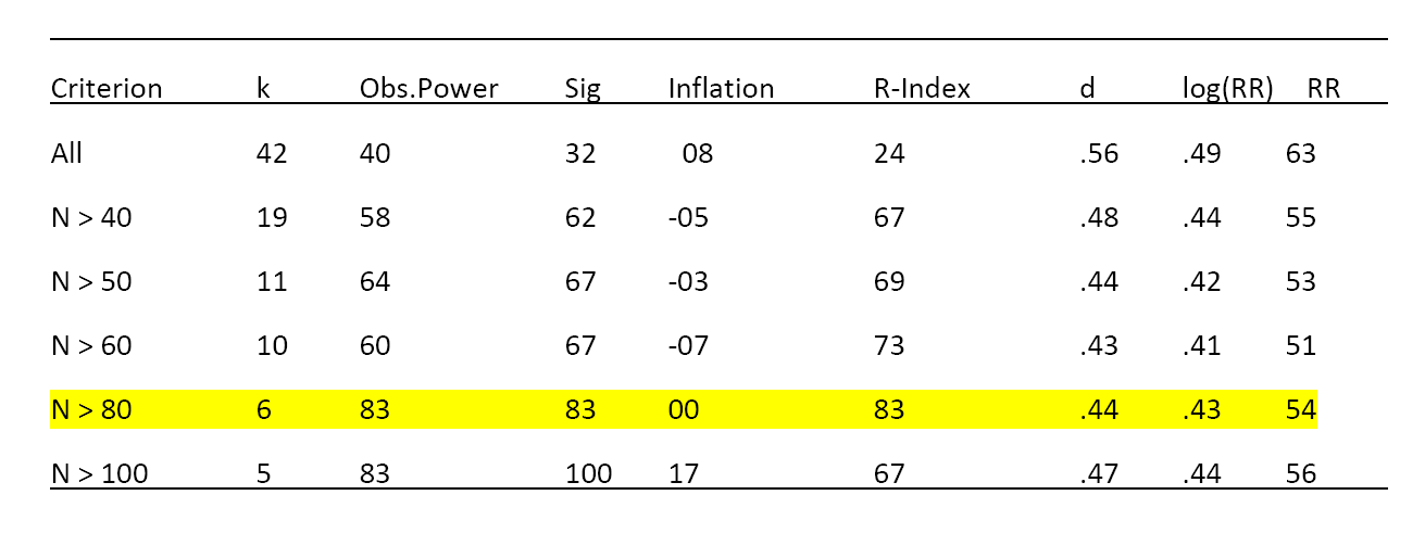
One possibility is that the existing studies vary in quality and that good studies showed the effect reliably, whereas bad studies failed to show the effect. To test this hypothesis, it is possible to select studies from a meta-analysis with the goal to maximize the R-Index. The best chance to obtain a high R-Index is to focus on studies with large sample sizes because statistical power increases with sample size. However, the table below shows that there are only 8 studies with more than 100 participants and the success rate in these studies is 13% (1 out of 8), which is consistent with the median observed power in these studies 12%.

R-IndexStereotypeThreatMetaAnalysis

It is also possible to select studies that produced significant results (z > 1.96). Of course, this set of studies is biased, but the R-Index corrects for bias. If these studies were successful because they had sufficient power to demonstrate effects, the R-Index would be greater than 50%. However, the R-Index is only 49%.

CONCLUSION

In conclusion, a replicability analysis with the R-Index shows that stereotype-threat is an elusive phenomenon. Even large replication studies with hundreds of participants were unable to provide evidence for an effect that appeared to be a robust effect in the original article. The R-Index of the meta-analysis by Flore and Wicherts corroborates concerns that the importance of stereotype-threat as an explanation for gender differences in math performance has been exaggerated. Similarly, Ganley, Mingle, Ryan, Ryan, and Vasilyeva (2013) found no evidence for stereotype threat effects in studies with 931 students and suggested that “these results raise the possibility that stereotype threat may not be the cause of gender differences in mathematics performance prior to college.” (p 1995).

The main novel contribution of this post is to reveal that this disappointing outcome was predicted on the basis of the empirical results reported in the original article by Spencer et al. (1999). The article suggested that stereotype threat is a pervasive phenomenon that explains gender differences in math performance. However, The R-Index and the insufficient variance in statistical results suggest that the reported results were biased and, overestimated the effect size of stereotype threat. The R-Index corrects for this bias and correctly predicts that replication studies will often result in non-significant results. The meta-analysis confirms this prediction.

In sum, the main conclusions that one can draw from 15 years of stereotype-threat research is that (a) the real reasons for gender differences in math performance are still unknown, (b) resources have been wasted in the pursuit of a negligible factor that may contribute to gender differences in math performance under very specific circumstances, and (c) that the R-Index could have prevented the irrational exuberance about stereotype-threat as a simple solution to an important social issue.

In a personal communication Dr. Spencer suggested that studies not included in the meta-analysis might produce different results. I suggested that Dr. Spencer provides a list of studies that provide empirical support for the hypothesis. A year later, Dr. Spencer has not provided any new evidence that provides credible evidence for stereotype-effects.  At present, the existing evidence suggests that published studies provide inflated estimates of the replicability and importance of the effect.

This blog also provides further evidence that male and female psychologists could benefit from a better education in statistics and research methods to avoid wasting resources in the pursuit of false-positive results.

How Power Analysis Could Have Prevented the Sad Story of Dr. Förster

[further information can be found in a follow up blog]

Background

In 2011, Dr. Förster published an article in Journal of Experimental Psychology: General. The article reported 12 studies and each study reported several hypothesis tests. The abstract reports that “In all experiments, global/local processing in 1 modality shifted to global/local processing in the other modality”.

For a while this article was just another article that reported a large number of studies that all worked and neither reviewers nor the editor who accepted the manuscript for publication found anything wrong with the reported results.

In 2012, an anonymous letter voiced suspicion that Jens Forster violated rules of scientific misconduct. The allegation led to an investigation, but as of today (January 1, 2015) there is no satisfactory account of what happened. Jens Förster maintains that he is innocent (5b. Brief von Jens Förster vom 10. September 2014) and blames the accusations about scientific misconduct on a climate of hypervigilance after the discovery of scientific misconduct by another social psychologist.

The Accusation

The accusation is based on an unusual statistical pattern in three publications. The 3 articles reported 40 experiments with 2284 participants, that is an average sample size of N = 57 participants in each experiment. The 40 experiments all had a between-subject design with three groups: one group received a manipulation design to increase scores on the dependent variable. A second group received the opposite manipulation to decrease scores on the dependent variable. And a third group served as a control condition with the expectation that the average of the group would fall in the middle of the two other groups. To demonstrate that both manipulations have an effect, both experimental groups have to show significant differences from the control group.

The accuser noticed that the reported means were unusually close to a linear trend. This means that the two experimental conditions showed markedly symmetrical deviations from the control group. For example, if one manipulation increased scores on the dependent variables by half a standard deviation (d = +.5), the other manipulation decreased scores on the dependent variable by half a standard deviation (d = -.5). Such a symmetrical pattern can be expected when the two manipulations are equally strong AND WHEN SAMPLE SIZES ARE LARGE ENOUGH TO MINIMIZE RANDOM SAMPLING ERROR. However, the sample sizes were small (n = 20 per condition, N = 60 per study). These sample sizes are not unusual and social psychologists often use n = 20 per condition to plan studies. However, these sample sizes have low power to produce consistent results across a large number of studies.

The accuser computed the statistical probability of obtaining the reported linear trend. The probability of obtaining the picture-perfect pattern of means by chance alone was incredibly small.

Based on this finding, the Dutch National Board for Research Integrity (LOWI) started an investigation of the causes for this unlikely finding. An English translation of the final report was published on retraction watch. An important question was whether the reported results could have been obtained by means of questionable research practices or whether the statistical pattern can only be explained by data manipulation. The English translation of the final report includes two relevant passages.

According to one statistical expert “QRP cannot be excluded, which in the opinion of the expert is a common, if not “prevalent” practice, in this field of science.” This would mean that Dr. Förster acted in accordance with scientific practices and that his behavior would not constitute scientific misconduct.

In response to this assessment the Complainant “extensively counters the expert’s claim that the unlikely patterns in the experiments can be explained by QRP.” This led to the decision that scientific misconduct occurred.

Four QRPs were considered.

  1. Improper rounding of p-values. This QRP can only be used rarely when p-values happen to be close to .05. It is correct that this QRP cannot produce highly unusual patterns in a series of replication studies. It can also be easily checked by computing exact p-values from reported test statistics.
  2. Selecting dependent variables from a set of dependent variables. The articles in question reported several experiments that used the same dependent variable. Thus, this QRP cannot explain the unusual pattern in the data.
  3. Collecting additional research data after an initial research finding revealed a non-significant result. This description of an QRP is ambiguous. Presumably it refers to optional stopping. That is, when the data trend in the right direction to continue data collection with repeated checking of p-values and stopping when the p-value is significant. This practices lead to random variation in sample sizes. However, studies in the reported articles all have more or less 20 participants per condition. Thus, optional stopping can be ruled out. However, if a condition with 20 participants does not produce a significant result, it could simply be discarded, and another condition with 20 participants could be run. With a false-positive rate of 5%, this procedure will eventually yield the desired outcome while holding sample size constant. It seems implausible that Dr. Förster conducted 20 studies to obtain a single significant result. Thus, it is even more plausible that the effect is actually there, but that studies with n = 20 per condition have low power. If power were just 30%, the effect would appear in every third study significantly, and only 60 participants were used to produce significant results in one out of three studies. The report provides insufficient information to rule out this QRP, although it is well-known that excluding failed studies is a common practice in all sciences.
  4. Selectively and secretly deleting data of participants (i.e., outliers) to arrive at significant results. The report provides no explanation how this QRP can be ruled out as an explanation. Simmons, Nelson, and Simonsohn (2011) demonstrated that conducting a study with 37 participants and then deleting data from 17 participants can contribute to a significant result when the null-hypothesis is true. However, if an actual effect is present, fewer participants need to be deleted to obtain a significant result. If the original sample size is large enough, it is always possible to delete cases to end up with a significant result. Of course, at some point selective and secretive deletion of observation is just data fabrication. Rather than making up data, actual data from participants are deleted to end up with the desired pattern of results. However, without information about the true effect size, it is difficult to determine whether an effect was present and just embellished (see Fisher’s analysis of Mendel’s famous genetics studies) or whether the null-hypothesis is true.

The English translation of the report does not contain any statements about questionable research practices from Dr. Förster. In an email communication on January 2, 2014, Dr. Förster revealed that he in fact ran multiple studies, some of which did not produce significant results, and that he only reported his best studies. He also mentioned that he openly admitted to this common practice to the commission. The English translation of the final report does not mention this fact. Thus, it remains an open question whether QRPs could have produced the unusual linearity in Dr. Förster’s studies.

A New Perspective: The Curse of Low Powered Studies

One unresolved question is why Dr. Förster would manipulate data to produce a linear pattern of means that he did not even mention in his articles. (Discover magazine).

One plausible answer is that the linear pattern is the by-product of questionable research practices to claim that two experimental groups with opposite manipulations are both significantly different from a control group. To support this claim, the articles always report contrasts of the experimental conditions and the control condition (see Table below). ForsterTable

In Table 1 the results of these critical tests are reported with subscripts next to the reported means. As the direction of the effect is theoretically determined, a one-tailed test was used. The null-hypothesis was rejected when p < .05.

Table 1 reports 9 comparisons of global processing conditions and control groups and 9 comparisons of local processing conditions with a control group; a total of 18 critical significance tests. All studies had approximately 20 participants per condition. The average effect size across the 18 studies is d = .71 (median d = .68).   An a priori power analysis with d = .7, N = 40, and significance criterion .05 (one-tailed) gives a power estimate of 69%.

An alternative approach is to compute observed power for each study and to use median observed power (MOP) as an estimate of true power. This approach is more appropriate when effect sizes vary across studies. In this case, it leads to the same conclusion, MOP = 67.

The MOP estimate of power implies that a set of 100 tests is expected to produce 67 significant results and 33 non-significant results. For a set of 18 tests, the expected values are 12.4 significant results and 5.6 non-significant results.

The actual success rate in Table 1 should be easy to infer from Table 1, but there are some inaccuracies in the subscripts. For example, Study 1a shows no significant difference between means of 38 and 31 (d = .60, but it shows a significant difference between means 31 and 27 (d = .33). Most likely the subscript for the control condition should be c not a.

Based on the reported means and standard deviations, the actual success rate with N = 40 and p < .05 (one-tailed) is 83% (15 significant and 3 non-significant results).

The actual success rate (83%) is higher than one would expect based on MOP (67%). This inflation in the success rate suggests that the reported results are biased in favor of significant results (the reasons for this bias are irrelevant for the following discussion, but it could be produced by not reporting studies with non-significant results, which would be consistent with Dr. Förster’s account ).

The R-Index was developed to correct for this bias. The R-Index subtracts the inflation rate (83% – 67% = 16%) from MOP. For the data in Table 1, the R-Index is 51% (67% – 16%).

Given the use of a between-subject design and approximately equal sample sizes in all studies, the inflation in power can be used to estimate inflation of effect sizes. A study with N = 40 and p < .05 (one-tailed) has 50% power when d = .50.

Thus, one interpretation of the results in Table 1 is that the true effect sizes of the manipulation is d = .5, that 9 out of 18 tests should have produced a significant contrast at p < .05 (one-tailed) and that questionable research practices were used to increase the success rate from 50% to 83% (15 vs. 9 successes).

The use of questionable research practices would also explain unusual linearity in the data. Questionable research practices will increase or omit effect sizes that are insufficient to produce a significant result. With a sample size of N = 40, an effect size of d = .5 is insufficient to produce a significant result, d = .5, se = 32, t(38) = 1.58, p = .06 (one-tailed). Random sampling error that works against the hypothesis can only produce non-significant results that have to be dropped or moved upwards using questionable methods. Random error that favors the hypothesis will inflate the effect size and start producing significant results. However, random error is normally distributed around the true effect size and is more likely to produce results that are just significant (d = .8) than to produce results that are very significant (d = 1.5). Thus, the reported effect sizes will be clustered more closely around the median inflated effect size than one would expect based on an unbiased sample of effect sizes.

The clustering of effect sizes will happen for the positive effects in the global processing condition and for the negative effects in the local processing condition. As a result, the pattern of all three means will be more linear than an unbiased set of studies would predict. In a large set of studies, this bias will produce a very low p-value.

One way to test this hypothesis is to examine the variability in the reported results. The Test of Insufficient Variance (TIVA) was developed for this purpose. TIVA first converts p-values into z-scores. The variance of z-scores is known to be 1. Thus, a representative sample of z-scores should have a variance of 1, but questionable research practices lead to a reduction in variance. The probability that a set of z-scores is a representative set of z-scores can be computed with a chi-square test and chi-square is a function of the ratio of the expected and observed variance and the number of studies. For the set of studies in Table 1, the variance in z-scores is .33. The chi-square value is 54. With 17 degrees of freedom, the p-value is 0.00000917 and the odds of this event occurring by chance are 1 out of 109,056 times.

Conclusion

Previous discussions about abnormal linearity in Dr. Förster’s studies have failed to provide a satisfactory answer. An anonymous accuser claimed that the data were fabricated or manipulated, which the author vehemently denies. This blog proposes a plausible explanation of what could have [edited January 19, 2015] happened. Dr. Förster may have conducted more studies than were reported and included only studies with significant results in his articles. Slight variation in sample sizes suggests that he may also have removed a few outliers selectively to compensate for low power. Importantly, neither of these practices would imply scientific misconduct. The conclusion of the commission that scientific misconduct occurred rests on the assumption that QRPs cannot explain the unusual linearity of means, but this blog points out how selective reporting of positive results may have inadvertently produced this linear pattern of means. Thus, the present analysis support the conclusion by an independent statistical expert mentioned in the LOWI report: “QRP cannot be excluded, which in the opinion of the expert is a common, if not “prevalent” practice, in this field of science.”

How Unusual is an R-Index of 51?

The R-Index for the 18 statistical tests reported in Table 1 is 51% and TIVA confirms that the reported p-values have insufficient variance. Thus, it is highly probable that questionable research practices contributed to the results and in a personal communication Dr. Förster confirmed that additional studies with non-significant results exist. However, in response to further inquiries [see follow up blog] Dr. Förster denied having used QRPs that could explain the linearity in his data.

Nevertheless, an R-Index of 51% is not unusual and has been explained with the use of QRPs.  For example, the R-Index for a set of studies by Roy Baumeister was 49%, . and Roy Baumeister stated that QRPs were used to obtain significant results.

“We did run multiple studies, some of which did not work, and some of which worked better than others. You may think that not reporting the less successful studies is wrong, but that is how the field works.”

Sadly, it is quite common to find an R-Index of 50% or lower for prominent publications in social psychology. This is not surprising because questionable research practices were considered good practices until recently. Even at present, it is not clear whether these practices constitute scientific misconduct (see discussion in Dialogue, Newsletter of the Society for Personality and Social Psychology).

How to Avoid Similar Sad Stories in the Future

One way to avoid accusations of scientific misconduct is to conduct a priori power analyses and to conduct only studies with a realistic chance to produce a significant result when the hypothesis is correct. When random error is small, true patterns in data can emerge without the help of QRPs.

Another important lesson from this story is to reduce the number of statistical tests as much as possible. Table 1 reported 18 statistical tests with the aim to demonstrate significance in each test. Even with a liberal criterion of .1 (one-tailed), it is highly unlikely that so many significant tests will produce positive results. Thus, a non-significant result is likely to emerge and researchers should think ahead of time how they would deal with non-significant results.

For the data in Table 1, Dr. Förster could have reported the means of 9 small studies without significance tests and conduct significance tests only once for the pattern in all 9 studies. With a total sample size of 360 participants (9 * 40), this test would have 90% power even if the effect size is only d = .35. With 90% power, the total power to obtain significant differences from the control condition for both manipulations would be 81%. Thus, the same amount of resources that were used for the controversial findings could have been used to conduct a powerful empirical test of theoretical predictions without the need to hide inconclusive, non-significant results in studies with low power.

Jacob Cohen has been trying to teach psychologists the importance of statistical power for decades and psychologists stubbornly ignored his valuable contribution to research methodology until he died in 1998. Methodologists have been mystified by the refusal of psychologists to increase power in their studies (Maxwell, 2004).

One explanation is that small samples provided a huge incentive. A non-significant result can be discarded with little cost of resources, whereas a significant result can be published and have the additional benefit of an inflated effect size, which allows boosting the importance of published results.

The R-Index was developed to balance the incentive structure towards studies with high power. A low R-Index reveals that a researcher is reporting biased results that will be difficult to replicate by other researchers. The R-Index reveals this inconvenient truth and lowers excitement about incredible results that are indeed incredible. The R-Index can also be used by researchers to control their own excitement about results that are mostly due to sampling error and to curb the excitement of eager research assistants that may be motivated to bias results to please a professor.

Curbed excitement does not mean that the R-Index makes science less exciting. Indeed, it will be exciting when social psychologists start reporting credible results about social behavior that boost a high R-Index because for a true scientist nothing is more exciting than the truth.

The R-Index of Nicotine-Replacement-Therapy Studies: An Alternative Approach to Meta-Regression

Stanley and Doucouliagos (2013) demonstrated how meta-regression can be used to obtain unbiased estimates of effect sizes from a biased set of original studies. The regression approach relies on the fact that small samples often need luck or questionable practices to produce significant results, whereas large samples can show true effects without the help of luck and questionable practices. If questionable practices or publication bias are present, effect sizes in small samples are inflated and this bias is evident in a regression of effect sizes on sampling error. When bias is present, the intercept of the regression equation can provide a better estimate of the average effect size in a set of studies.

One limitation of this approach is that other factors can also produce a correlation between effect size and sampling error. Another problem is that the regression equation can only approximate the effect of bias on effect size estimates.

The R-Index can complement meta-regression in several ways. First, it can be used to examine whether a correlation between effect size and sampling error reflects bias. If small samples have higher effect sizes due to bias, they should also yield more significant results than the power of these studies justifies. If this is not the case, the correlation may simply show that smaller samples examined stronger effects. Second, the R-Index can be used as an alternative way to estimate unbiased effect sizes that does not rely on the relationship between sample size and effect size.

The usefulness of the R-Index is illustrated with Stanley and Doucouliagos (2013) meta-analysis of the effectiveness of nicotine replacement therapy (the patch). Table A1 lists sampling errors and t-values of 42 studies. Stanley and Doucouliagos (2013) found that the 42 studies suggested a reduction in smoking by 93%, but that effectiveness decreased to 22% in a regression that controlled for biased reporting of results. This suggests that published studies inflate the true effect by more than 300%.

I entered the t-values and standard errors into the R-Index spreadsheet. I used sampling error to estimate sample sizes and degrees of freedom (2 / sqrt [N]). I used one-tailed t-tests to allow for negative t-values because the sign of effects is known in a meta-analysis of studies that try to show treatment effects. Significance was tested using p = .025, which is equivalent to using .050 in the test of significance for two-tailed tests (z > 1.96).

The R-Index for all 42 studies was 27%. The low R-Index was mostly explained by the low power of studies with small samples. Median observed power was just 34%. The number of significant results was only slightly higher 40%. The inflation rate was only 7%.

As studies with low power add mostly noise, Stanley (2010) showed that it can be preferable to exclude them from estimates of actual effect sizes. The problem is that it is difficult to find a principled way to determine which studies should be included or excluded. One solution is to retain only studies with large samples. The problem with this approach is that this often limits a meta-analysis to a small set of studies.

One solution is to compute the R-Index for different sets of studies and to base conclusions on the largest unbiased set of studies. For the 42 studies of nicotine replacement therapy, the following effect size estimates were obtained (effect sizes are d-values, d = t * se).

NicotinePatch

The results show the highest R-Index for studies with more than 80 participants. For these studies, observed power is 83% and the percentage of significant results is also 83%, suggesting that this set of studies is an unbiased sample of studies. The weighted average effect size for this set of studies is d = .44. The results also show that the weighted average effect size does not change much as a function of the selection of studies. When all studies are included, there is evidence of bias (8% inflation) and the weighted average effect size is inflated, but the amount of inflation is small (d = .56 vs. d = .44, difference d = .12).

The small amount of bias appears to be inconsistent with Stanley and Doucouliagos (2013) estimate that an uncorrected meta-analysis overestimates the true effect size by over 300% (93% vs. 22% RR). I therefore also examined the log(RR) values in Table 1a.

The average is .68 (compared to the simple mean reported as .66); the median is .53 and the weighted average is .49.   The regression-corrected estimate reported by Stanley and Doucouliagos (2013) is .31. The weighted mean for studies with more than 80 participants is .43. It is now clear why Stanley and Doucouliagos (2013) reported a large effect of the bias correction. First, they used the simple mean as a comparison standard (.68 vs. 31). The effect would be smaller if they had used the weighted mean as a comparison standard (.49 vs. .31). Another factor is that the regression procedure produces a lower estimate than the R-Index approach (.31 vs. 43). More research is needed to compare these results, but the R-Index has a simple logic. When there is no evidence of bias, the weighted average provides a reasonable estimate of the true effect size.

Conclusion

Stanley and Doucouliagos (2013) used regression of effect sizes on sampling error to reveal biases and to obtain an unbiased estimate of the typical effect size in a set of studies. This approach provides a useful tool in the fight against biased reporting of research results. One limitation of this approach is that other factors can produce a correlation between sampling error and effect size. The R-Index can be used to examine how much reporting biases contribute to this correlation. The R-Index can also be used to obtain an unbiased estimate of effect size by computing a weighted average for a select set of studies with a high R-Index.

A meta-analysis of 42 studies of nicotine replacement theory illustrates this approach. The R-Index for the full set of studies was low (24%). This reveals that many studies had low power to demonstrate an effect. These studies provide little information about effectiveness because non-significant results are just as likely to be type-II errors as demonstrations of low effectiveness.

The R-Index increased when studies with larger samples were selected. The maximum R-Index was obtained for studies with at least 80 participants. In this case, observed power was above 80% and there was no evidence of bias. The weighted average effect size for this set of studies was only slightly lower than the weighted average effect size for all studies (log(RR) = .43 vs. .49, RR = 54% vs. 63%, respectively). This finding suggests that smokers who use a nicotine patch are about 50% more likely to quit smoking than smokers without a nicotine patch.

The estimate of 50% risk reduction challenges Stanley and Doucouliagos’s (2013) preferred estimate that bias correction “reduces the efficacy of the patch to only 22%.” The R-Index suggests that this bias-corrected estimate is itself biased.

Another important conclusion is that studies with low power are wasteful and uninformative. They generate a lot of noise and are likely to be systematically biased and they contribute little to a meta-analysis that weights studies by sample size. The best estimate of effect size was based on only 6 out of 42 studies. Researchers should not conduct studies with low power and editors should not publish studies with low power.