Category Archives: Replicability

REPLICABILITY RANKING OF 26 PSYCHOLOGY JOURNALS

THEORETICAL BACKGROUND

Neyman & Pearson (1933) developed the theory of type-I and type-II errors in statistical hypothesis testing.

A type-I error is defined as the probability of rejecting the null-hypothesis (i.e., the effect size is zero) when the null-hypothesis is true.

A type-II error is defined as the probability of failing to reject the null-hypothesis when the null-hypothesis is false (i.e., there is an effect).

A common application of statistics is to provide empirical evidence for a theoretically predicted relationship between two variables (cause-effect or covariation). The results of an empirical study can produce two outcomes. Either the result is statistically significant or it is not statistically significant. Statistically significant results are interpreted as support for a theoretically predicted effect.

Statistically non-significant results are difficult to interpret because the prediction may be false (the null-hypothesis is true) or a type-II error occurred (the theoretical prediction is correct, but the results fail to provide sufficient evidence for it).

To avoid type-II errors, researchers can design studies that reduce the type-II error probability. The probability of avoiding a type-II error when a predicted effect exists is called power. It could also be called the probability of success because a significant result can be used to provide empirical support for a hypothesis.

Ideally researchers would want to maximize power to avoid type-II errors. However, powerful studies require more resources. Thus, researchers face a trade-off between the allocation of resources and their probability to obtain a statistically significant result.

Jacob Cohen dedicated a large portion of his career to help researchers with the task of planning studies that can produce a successful result, if the theoretical prediction is true. He suggested that researchers should plan studies to have 80% power. With 80% power, the type-II error rate is still 20%, which means that 1 out of 5 studies in which a theoretical prediction is true would fail to produce a statistically significant result.

Cohen (1962) examined the typical effect sizes in psychology and found that the typical effect size for the mean difference between two groups (e.g., men and women or experimental vs. control group) is about half-of a standard deviation. The standardized effect size measure is called Cohen’s d in his honor. Based on his review of the literature, Cohen suggested that an effect size of d = .2 is small, d = .5 moderate, and d = .8. Importantly, a statistically small effect size can have huge practical importance. Thus, these labels should not be used to make claims about the practical importance of effects. The main purpose of these labels is that researchers can better plan their studies. If researchers expect a large effect (d = .8), they need a relatively small sample to have high power. If researchers expect a small effect (d = .2), they need a large sample to have high power.   Cohen (1992) provided information about effect sizes and sample sizes for different statistical tests (chi-square, correlation, ANOVA, etc.).

Cohen (1962) conducted a meta-analysis of studies published in a prominent psychology journal. Based on the typical effect size and sample size in these studies, Cohen estimated that the average power in studies is about 60%. Importantly, this also means that the typical power to detect small effects is less than 60%. Thus, many studies in psychology have low power and a high type-II error probability. As a result, one would expect that journals often report that studies failed to support theoretical predictions. However, the success rate in psychological journals is over 90% (Sterling, 1959; Sterling, Rosenbaum, & Weinkam, 1995). There are two explanations for discrepancies between the reported success rate and the success probability (power) in psychology. One explanation is that researchers conduct multiple studies and only report successful studies. The other studies remain unreported in a proverbial file-drawer (Rosenthal, 1979). The other explanation is that researchers use questionable research practices to produce significant results in a study (John, Loewenstein, & Prelec, 2012). Both practices have undesirable consequences for the credibility and replicability of published results in psychological journals.

A simple solution to the problem would be to increase the statistical power of studies. If the power of psychological studies in psychology were over 90%, a success rate of 90% would be justified by the actual probability of obtaining significant results. However, meta-analysis and method articles have repeatedly pointed out that psychologists do not consider statistical power in the planning of their studies and that studies continue to be underpowered (Maxwell, 2004; Schimmack, 2012; Sedlmeier & Giegerenzer, 1989).

One reason for the persistent neglect of power could be that researchers have no awareness of the typical power of their studies. This could happen because observed power in a single study is an imperfect indicator of true power (Yuan & Maxwell, 2005). If a study produced a significant result, the observed power is at least 50%, even if the true power is only 30%. Even if the null-hypothesis is true, and researchers publish only type-I errors, observed power is dramatically inflated to 62%, when the true power is only 5% (the type-I error rate). Thus, Cohen’s estimate of 60% power is not very reassuring.

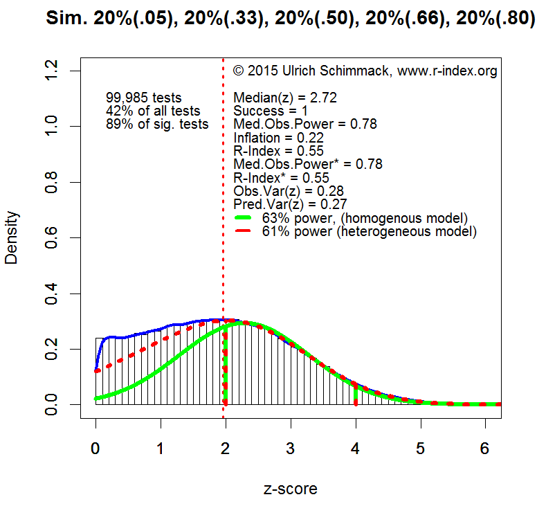
Over the past years, Schimmack and Brunner have developed a method to estimate power for sets of studies with heterogeneous designs, sample sizes, and effect sizes. A technical report is in preparation. The basic logic of this approach is to convert results of all statistical tests into z-scores using the one-tailed p-value of a statistical test.  The z-scores provide a common metric for observed statistical results. The standard normal distribution predicts the distribution of observed z-scores for a fixed value of true power.   However, for heterogeneous sets of studies the distribution of z-scores is a mixture of standard normal distributions with different weights attached to various power values. To illustrate this method, the histograms of z-scores below show simulated data with 10,000 observations with varying levels of true power: 20% null-hypotheses being true (5% power), 20% of studies with 33% power, 20% of studies with 50% power, 20% of studies with 66% power, and 20% of studies with 80% power.
RepRankSimulation

The plot shows the distribution of absolute z-scores (there are no negative effect sizes). The plot is limited to z-scores below 6 (N = 99,985 out of 10,000). Z-scores above 6 standard deviations from zero are extremely unlikely to occur by chance. Even with a conservative estimate of effect size (lower bound of 95% confidence interval), observed power is well above 99%. Moreover, quantum physics uses Z = 5 as a criterion to claim success (e.g., discovery of Higgs-Boson Particle). Thus, Z-scores above 6 can be expected to be highly replicable effects.

Z-scores below 1.96 (the vertical dotted red line) are not significant for the standard criterion of (p < .05, two-tailed). These values are excluded from the calculation of power because these results are either not reported or not interpreted as evidence for an effect. It is still important to realize that true power of all experiments would be lower if these studies were included because many of the non-significant results are produced by studies with 33% power. These non-significant results create two problems. Researchers wasted resources on studies with inconclusive results and readers may be tempted to misinterpret these results as evidence that an effect does not exist (e.g., a drug does not have side effects) when an effect is actually present. In practice, it is difficult to estimate power for non-significant results because the size of the file-drawer is difficult to estimate.

It is possible to estimate power for any range of z-scores, but I prefer the range of z-scores from 2 (just significant) to 4. A z-score of 4 has a 95% confidence interval that ranges from 2 to 6. Thus, even if the observed effect size is inflated, there is still a high chance that a replication study would produce a significant result (Z > 2). Thus, all z-scores greater than 4 can be treated as cases with 100% power. The plot also shows that conclusions are unlikely to change by using a wider range of z-scores because most of the significant results correspond to z-scores between 2 and 4 (89%).

The typical power of studies is estimated based on the distribution of z-scores between 2 and 4. A steep decrease from left to right suggests low power. A steep increase suggests high power. If the peak (mode) of the distribution were centered over Z = 2.8, the data would conform to Cohen’s recommendation to have 80% power.

Using the known distribution of power to estimate power in the critical range gives a power estimate of 61%. A simpler model that assumes a fixed power value for all studies produces a slightly inflated estimate of 63%. Although the heterogeneous model is correct, the plot shows that the homogeneous model provides a reasonable approximation when estimates are limited to a narrow range of Z-scores. Thus, I used the homogeneous model to estimate the typical power of significant results reported in psychological journals.

DATA

The results presented below are based on an ongoing project that examines power in psychological journals (see results section for the list of journals included so far). The set of journals does not include journals that primarily publish reviews and meta-analysis or clinical and applied journals. The data analysis is limited to the years from 2009 to 2015 to provide information about the typical power in contemporary research. Results regarding historic trends will be reported in a forthcoming article.

I downloaded pdf files of all articles published in the selected journals and converted the pdf files to text files. I then extracted all t-tests and F-tests that were reported in the text of the results section searching for t(df) or F(df1,df2). All t and F statistics were converted into one-tailed p-values and then converted into z-scores.

RepRankAll

The plot above shows the results based on 218,698 t and F tests reported between 2009 and 2015 in the selected psychology journals. Unlike the simulated data, the plot shows a steep drop for z-scores just below the threshold of significance (z = 1.96). This drop is due to the tendency not to publish or report non-significant results. The heterogeneous model uses the distribution of non-significant results to estimate the size of the file-drawer (unpublished non-significant results). However, for the present purpose the size of the file-drawer is irrelevant because power is estimated only for significant results for Z-scores between 2 and 4.

The green line shows the best fitting estimate for the homogeneous model. The red curve shows fit of the heterogeneous model. The heterogeneous model is doing a much better job at fitting the long tail of highly significant results, but for the critical interval of z-scores between 2 and 4, the two models provide similar estimates of power (55% homogeneous & 53% heterogeneous model).   If the range is extended to z-scores between 2 and 6, power estimates diverge (82% homogenous, 61% heterogeneous). The plot indicates that the heterogeneous model fits the data better and that the 61% estimate is a better estimate of true power for significant results in this range. Thus, the results are in line with Cohen (1962) estimate that psychological studies average 60% power.

REPLICABILITY RANKING

The distribution of z-scores between 2 and 4 was used to estimate the average power separately for each journal. As power is the probability to obtain a significant result, this measure estimates the replicability of results published in a particular journal if researchers would reproduce the studies under identical conditions with the same sample size (exact replication). Thus, even though the selection criterion ensured that all tests produced a significant result (100% success rate), the replication rate is expected to be only about 50%, even if the replication studies successfully reproduce the conditions of the published studies. The table below shows the replicability ranking of the journals, the replicability score, and a grade. Journals are graded based on a scheme that is similar to grading schemes for undergraduate students (below 50 = F, 50-59 = E, 60-69 = D, 70-79 = C, 80-89 = B, 90+ = A).

ReplicabilityRanking

The average value in 2000-2014 is 57 (D+). The average value in 2015 is 58 (D+). The correlation for the values in 2010-2014 and those in 2015 is r = .66.   These findings show that the replicability scores are reliable and that journals differ systematically in the power of published studies.

LIMITATIONS

The main limitation of the method is that focuses on t and F-tests. The results might change when other statistics are included in the analysis. The next goal is to incorporate correlations and regression coefficients.

The second limitation is that the analysis does not discriminate between primary hypothesis tests and secondary analyses. For example, an article may find a significant main effect for gender, but the critical test is whether gender interacts with an experimental manipulation. It is possible that some journals have lower scores because they report more secondary analyses with lower power. To address this issue, it will be necessary to code articles in terms of the importance of statistical test.

The ranking for 2015 is based on the currently available data and may change when more data become available. Readers should also avoid interpreting small differences in replicability scores as these scores are likely to fluctuate. However, the strong correlation over time suggests that there are meaningful differences in the replicability and credibility of published results across journals.

CONCLUSION

This article provides objective information about the replicability of published findings in psychology journals. None of the journals reaches Cohen’s recommended level of 80% replicability. Average replicability is just about 50%. This finding is largely consistent with Cohen’s analysis of power over 50 years ago. The publication of the first replicability analysis by journal should provide an incentive to editors to increase the reputation of their journal by paying more attention to the quality of the published data. In this regard, it is noteworthy that replicability scores diverge from traditional indicators of journal prestige such as impact factors. Ideally, the impact of an empirical article should be aligned with the replicability of the empirical results. Thus, the replicability index may also help researchers to base their own research on credible results that are published in journals with a high replicability score and to avoid incredible results that are published in journals with a low replicability score. Ultimately, I can only hope that journals will start competing with each other for a top spot in the replicability rankings and as a by-product increase the replicability of published findings and the credibility of psychological science.

Why are Stereotype-Threat Effects on Women’s Math Performance Difficult to Replicate?

Updated on May 19, 2016
– corrected mistake in calculation of p-value for TIVA

A Replicability Analysis of Spencer, Steele, and Quinn’s seminal article on stereotype threat effects on gender differences in math performance.

Background

In a seminal article, Spencer, Steele, and Quinn (1999) proposed the concept of stereotype threat. They argued that women may experience stereotype-threat during math tests and that stereotype threat can interfere with their performance on math tests.

The original study reported three experiments.

STUDY 1

Study 1 had 56 participants (28 male and 28 female undergraduate students). The main aim was to demonstrate that stereotype-threat influences performance on difficult, but not on easy math problems.

A 2 x 2 mixed model ANOVA with sex and difficulty produced the following results.

Main effect for sex, F(1, 52) = 3.99, p = .051 (reported as p = .05), z = 1.96, observed power = 50%.

Interaction between sex and difficulty, F(1, 52) = 5.34 , p = .025, z = 2.24, observed power = 61%.

The low observed power suggests that sampling error contributed to the significant results. Assuming observed power is a reliable estimate of true power, the chance of obtaining significant results in both studies would only be 31%. Moreover, if the true power is in the range between 50% and 80% power, there is only a 32% chance that observed power to fall into this range. The chance that both observed power values fall into this range is only 10%.

Median observed power is 56%. The success rate is 100%. Thus, the success rate is inflated by 44 percentage points (100% – 56%).

The R-Index for these two results is low, Ř = 12 (56 – 44).

Empirical evidence shows that studies with low R-Indices often fail to replicate in exact replication studies.

It is even more problematic that Study 1 was supposed to demonstrate just the basic phenomenon that women perform worse on math problems than men and that the following studies were designed to move this pre-existing gender difference around with an experimental manipulation. If the actual phenomenon is in doubt, it is unlikely that experimental manipulations of the phenomenon will be successful.

STUDY 2

The main purpose of Study 2 was to demonstrate that gender differences in math performance would disappear when the test is described as gender neutral.

Study 2 recruited 54 students (30 women, 24 men). This small sample size is problematic for several reasons. Power analysis of Study 1 suggested that the authors were lucky to obtain significant results. If power is 50%, there is a 50% chance that an exact replication study with the same sample size will produce a non-significant result. Another problem is that sample sizes need to increase to demonstrate that the gender difference in math performance can be influenced experimentally.

The data were not analyzed according to this research plan because the second test was so difficult that nobody was able to solve these math problems. However, rather than repeating the experiment with a better selection of math problems, the results for the first math test were reported.

As there was no repeated performance by the two participants, this is a 2 x 2 between-subject design that crosses sex and treat-manipulation. With a total sample size of 54 students, the n per cell is 13.

The main effect for sex was significant, F(1, 50) = 5.66, p = .021, z = 2.30, observed power = 63%.

The interaction was also significant, F(1, 50) = 4.18, p = .046, z = 1.99, observed power = 51%.

Once more, median observed power is just 57%, yet the success rate is 100%. Thus, the success rate is inflated by 43% and the R-Index is low, Ř = 14%, suggesting that an exact replication study will not produce significant results.

STUDY 3

Studies 1 and 2 used highly selective samples (women in the top 10% in math performance). Study 3 aimed to replicate the results of Study 2 in a less selective sample. One might expect that stereotype-threat has a weaker effect on math performance in this sample because stereotype threat can undermine performance when ability is high, but anxiety is not a factor in performance when ability is low. Thus, Study 3 is expected to yield a weaker effect and a larger sample size would be needed to demonstrate the effect. However, sample size was approximately the same as in Study 2 (36 women, 31 men).

The ANOVA showed a main effect of sex on math performance, F(1, 63) = 6.44, p = .014, z = 2.47, observed power = 69%.

The ANOVA also showed a significant interaction between sex and stereotype-threat-assurance, F(1, 63) = 4.78, p = .033, z = 2.14, observed power = 57%.

Once more, the R-Index is low, Ř = 26 (MOP = 63%, Success Rate = 100%, Inflation Rate = 37%).

Combined Analysis

The three studies reported six statistical tests. The R-Index for the combined analysis is low Ř = 18 (MOP = 59%, Success Rate = 100%, Inflation Rate = 41%).

The probability of this event to occur by chance can be assessed with the Test of Insufficient Variance (TIVA). TIVA tests the hypothesis that the variance in p-values, converted into z-scores, is less than 1. A variance of one is expected in a set of exact replication studies with fixed true power. Less variance suggests that the z-scores are not a representative sample of independent test scores.   The variance of the six z-scores is low, Var(z) = .04, p < .001,  1 / 1309.

Correction: I initially reported, “A chi-square test shows that the probability of this event is less than 1 out of 1,000,000,000,000,000, chi-square (df = 5) = 105.”

I made a mistake in the computation of the probability. When I developed TIVA, I confused the numerator and denominator in the test. I was thrilled that the test was so powerful and happy to report the result in bold, but it is incorrect. A small sample of six z-scores cannot produce such low p-values.

Conclusion

The replicability analysis of Spencer, Steele, and Quinn (1999) suggests that the original data provided inflated estimates of effect sizes and replicability. Thus, the R-Index predicts that exact replication studies would fail to replicate the effect.

Meta-Analysis

A forthcoming article in the Journal of School Psychology reports the results of a meta-analysis of stereotype-threat studies in applied school settings (Flore & Wicherts, 2014). The meta-analysis was based on 47 comparisons of girls with stereotype threat versus girls without stereotype threat. The abstract concludes that stereotype threat in this population is a statistically reliable, but small effect (d = .22). However, the authors also noted signs of publication bias. As publication bias inflates effect sizes, the true effect size is likely to be even smaller than the uncorrected estimate of .22.

The article also reports that the after a correction for bias, using the trim-and-fill method, the estimated effect size is d = .07 and not significantly different from zero. Thus, the meta-analysis reveals that there is no replicable evidence for stereotype-threat effects on schoolgirls’ math performance. The meta-analysis also implies that any true effect of stereotype threat is likely to be small (d < .2). With a true effect size of d = .2, the original studies by Steel et al. (1999) and most replication studies had insufficient power to demonstrate stereotype threat effects, even if the effect exists. A priori power analysis with d = .2 would suggest that 788 participants are needed to have an 80% chance to obtain a significant result if the true effect is d = .2. Thus, future research on this topic is futile unless statistical power is increased by increasing sample sizes or by using more powerful designs that can demonstrate small effects in smaller samples.

One possibility is that the existing studies vary in quality and that good studies showed the effect reliably, whereas bad studies failed to show the effect. To test this hypothesis, it is possible to select studies from a meta-analysis with the goal to maximize the R-Index. The best chance to obtain a high R-Index is to focus on studies with large sample sizes because statistical power increases with sample size. However, the table below shows that there are only 8 studies with more than 100 participants and the success rate in these studies is 13% (1 out of 8), which is consistent with the median observed power in these studies 12%.

R-IndexStereotypeThreatMetaAnalysis

It is also possible to select studies that produced significant results (z > 1.96). Of course, this set of studies is biased, but the R-Index corrects for bias. If these studies were successful because they had sufficient power to demonstrate effects, the R-Index would be greater than 50%. However, the R-Index is only 49%.

CONCLUSION

In conclusion, a replicability analysis with the R-Index shows that stereotype-threat is an elusive phenomenon. Even large replication studies with hundreds of participants were unable to provide evidence for an effect that appeared to be a robust effect in the original article. The R-Index of the meta-analysis by Flore and Wicherts corroborates concerns that the importance of stereotype-threat as an explanation for gender differences in math performance has been exaggerated. Similarly, Ganley, Mingle, Ryan, Ryan, and Vasilyeva (2013) found no evidence for stereotype threat effects in studies with 931 students and suggested that “these results raise the possibility that stereotype threat may not be the cause of gender differences in mathematics performance prior to college.” (p 1995).

The main novel contribution of this post is to reveal that this disappointing outcome was predicted on the basis of the empirical results reported in the original article by Spencer et al. (1999). The article suggested that stereotype threat is a pervasive phenomenon that explains gender differences in math performance. However, The R-Index and the insufficient variance in statistical results suggest that the reported results were biased and, overestimated the effect size of stereotype threat. The R-Index corrects for this bias and correctly predicts that replication studies will often result in non-significant results. The meta-analysis confirms this prediction.

In sum, the main conclusions that one can draw from 15 years of stereotype-threat research is that (a) the real reasons for gender differences in math performance are still unknown, (b) resources have been wasted in the pursuit of a negligible factor that may contribute to gender differences in math performance under very specific circumstances, and (c) that the R-Index could have prevented the irrational exuberance about stereotype-threat as a simple solution to an important social issue.

In a personal communication Dr. Spencer suggested that studies not included in the meta-analysis might produce different results. I suggested that Dr. Spencer provides a list of studies that provide empirical support for the hypothesis. A year later, Dr. Spencer has not provided any new evidence that provides credible evidence for stereotype-effects.  At present, the existing evidence suggests that published studies provide inflated estimates of the replicability and importance of the effect.

This blog also provides further evidence that male and female psychologists could benefit from a better education in statistics and research methods to avoid wasting resources in the pursuit of false-positive results.

The Test of Insufficient Variance (TIVA): A New Tool for the Detection of Questionable Research Practices

Citation. Schimmack, U. (2015). The Test of Insufficient
Variance (TIVA): A new tool for the detection of questionable research practices. Retrieved from http:// replicationindex.wordpress.com/2015/01/01/tiva

Updated 2025/08/20
I never submitted this work for peer-review, but the method has been reviewed in a peer-reviewed article and compared to other bias detection tools. Like many other tests, it does not work well when heterogeneity in effect sizes or sample sizes (or both) produces heterogeneity in power, but it did really well when all studies tested similar effect sizes which is often the case when they are small or zero.

Renkewitz, F., & Keiner, M. (2019). How to detect publication bias in psychological research: A comparative evaluation of six statistical methods. Zeitschrift für Psychologie, 227(4), 261–279. https://doi.org/10.1027/2151-2604/a000386

The Test of Insufficient Variance

It has been known for decades that published results tend to be biased (Sterling, 1959). For most of the past decades this inconvenient truth has been ignored. In the past years, there have been many suggestions and initiatives to increase the replicability of reported scientific findings (Asendorpf et al., 2013). One approach is to examine published research results for evidence of questionable research practices (see Schimmack, 2014, for a discussion of existing tests). This blog post introduces a new test of bias in reported research findings, namely the Test of Insufficient Variance (TIVA).

TIVA is applicable to any set of studies that used null-hypothesis testing to conclude that empirical data provide support for an empirical relationship and reported a significance test (p-values).

Rosenthal (1978) developed a method to combine results of several independent studies by converting p-values into z-scores. This conversion uses the well-known fact that p-values correspond to the area under the curve of a normal distribution. Rosenthal did not discuss the relation between these z-scores and power analysis. Z-scores are observed scores that should follow a normal distribution around the non-centrality parameter that determines how much power a study has to produce a significant result. In the Figure, the non-centrality parameter is 2.2. This value is slightly above a z-score of 1.96, which corresponds to a two-tailed p-value of .05. A study with a non-centrality parameter of 2.2 has 60% power.  In specific studies, the observed z-scores vary as a function of random sampling error. The standardized normal distribution predicts the distribution of observed z-scores. As observed z-scores follow the standard normal distribution, the variance of an unbiased set of z-scores is 1.  The Figure on top illustrates this with the nine purple lines, which are nine randomly generated z-scores with a variance of 1.

In a real data set the variance can be greater than 1 for two reasons. First, if the nine studies are exact replication studies with different sample sizes, larger samples will have a higher non-centrality parameter than smaller samples. This variance in the true non-centrality variances adds to the variance produced by random sampling error. Second, a set of studies that are not exact replication studies can have variance greater than 1 because the true effect sizes can vary across studies. Again, the variance in true effect sizes produces variance in the true non-centrality parameters that add to the variance produced by random sampling error.  In short, the variance is 1 in exact replication studies that also hold the sample size constant. When sample sizes and true effect sizes vary, the variance in observed z-scores is greater than 1. Thus, an unbiased set of z-scores should have a minimum variance of 1.

If the variance in z-scores is less than 1, it suggests that the set of z-scores is biased. One simple reason for insufficient variance is publication bias. If power is 50% and the non-centrality parameter matches the significance criterion of 1.96, 50% of studies that were conducted would not be significant. If these studies are omitted from the set of studies, variance decreases from 1 to .36. Another reason for insufficient variance is that researchers do not report non-significant results or used questionable research practices to inflate effect size estimates. The effect is that variance in observed z-scores is restricted.  Thus, insufficient variance in observed z-scores reveals that the reported results are biased and provide an inflated estimate of effect size and replicability.

In small sets of studies, insufficient variance may be due to chance alone. It is possible to quantify how lucky a researcher was to obtain significant results with insufficient variance. This probability is a function of two parameters: (a) the ratio of the observed variance (OV) in a sample over the population variance (i.e., 1), and (b) the number of z-scores minus 1 as the degrees of freedom (k -1).

The product of these two parameters follows a chi-square distribution with k-1 degrees of freedom.

Formula 1: Chi-square = OV * (k – 1) with k-1 degrees of freedom.

Example 1:

Bem (2011) published controversial evidence that appear to demonstrate precognition. Subsequent studies failed to replicate these results (Galak et al.,, 2012) and other bias tests show evidence that the reported results are biased Schimmack (2012). For this reason, Bem’s article provides a good test case for TIVA.

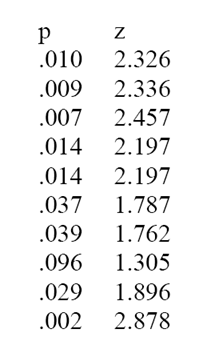
Bem_p_ZThe article reported results of 10 studies with 9 z-scores being significant at p < .05 (one-tailed). The observed variance in the 10 z-scores is 0.19. Using Formula 1, the chi-square value is chi^2 (df = 9) = 1.75. Importantly, chi-square tests are usually used to test whether variance is greater than expected by chance (right tail of the distribution). The reason is that variance is not expected to be less than the variance expected by chance because it is typically assumed that a set of data is unbiased. To obtain a probability of insufficient variance, it is necessary to test the left-tail of the chi-square distribution.  The corresponding p-value for chi^2 (df = 9) = 1.75 is p = .005. Thus, there is only a 1 out of 200 probability that a random set of 10 studies would produce a variance as low as Var = .19.

This outcome cannot be attributed to publication bias because all studies were published in a single article. Thus, TIVA supports the hypothesis that the insufficient variance in Bem’s z-scores is the result of questionable research methods and that the reported effect size of d = .2 is inflated. The presence of bias does not imply that the true effect size is 0, but it does strongly suggest that the true effect size is smaller than the average effect size in a set of studies with insufficient variance.

Example 2:  

Vohs et al. (2006) published a series of studies that he results of nine experiments in which participants were reminded of money. The results appeared to show that “money brings about a self-sufficient orientation.” Francis and colleagues suggested that the reported results are too good to be true. An R-Index analysis showed an R-Index of 21, which is consistent with a model in which the null-hypothesis is true and only significant results are reported.

Because Vohs et al. (2006) conducted multiple tests in some studies, the median p-value was used for conversion into z-scores. The p-values and z-scores for the nine studies are reported in Table 2. The Figure on top of this blog illustrates the distribution of the 9 z-scores relative to the expected standard normal distribution.

Table 2

Study                    p             z          

Study 1                .026       2.23
Study 2                .050       1.96
Study 3                .046       1.99
Study 4                .039       2.06
Study 5                .021       2.99
Study 6                .040       2.06
Study 7                .026       2.23
Study 8                .023       2.28
Study 9                .006       2.73
                                                           

The variance of the 9 z-scores is .054. This is even lower than the variance in Bem’s studies. The chi^2 test shows that this variance is significantly less than expected from an unbiased set of studies, chi^2 (df = 8) = 1.12, p = .003. An unusual event like this would occur in only 1 out of 381 studies by chance alone.

In conclusion, insufficient variance in z-scores shows that it is extremely likely that the reported results overestimate the true effect size and replicability of the reported studies. This confirms earlier claims that the results in this article are too good to be true (Francis et al., 2014). However, TIVA is more powerful than the Test of Excessive Significance and can provide more conclusive evidence that questionable research practices were used to inflate effect sizes and the rate of significant results in a set of studies.

Conclusion

TIVA can be used to examine whether a set of published p-values was obtained with the help of questionable research practices. When p-values are converted into z-scores, the variance of z-scores should be greater or equal to 1. Insufficient variance suggests that questionable research practices were used to avoid publishing non-significant results; this includes simply not reporting failed studies.

At least within psychology, these questionable research practices are used frequently to compensate for low statistical power and they are not considered scientific misconduct by governing bodies of psychological science (APA, APS, SPSP). Thus, the present results do not imply scientific misconduct by Bem or Vohs, just like the use of performance enhancing drugs in sports is not illegal unless a drug is put on an anti-doping list. However, jut because a drug is not officially banned, it does not mean that the use of a drug has no negative effects on a sport and its reputation.

One limitation of TIVA is that it requires a set of studies and that variance in small sets of studies can vary considerably just by chance. Another limitation is that TIVA is not very sensitive when there is substantial heterogeneity in true non-centrality parameters. In this case, the true variance in z-scores can mask insufficient variance in random sampling error. For this reason, TIVA is best used in conjunction with other bias tests. Despite these limitations, the present examples illustrate that TIVA can be a powerful tool in the detection of questionable research practices.  Hopefully, this demonstration will lead to changes in the way researchers view questionable research practices and how the scientific community evaluates results that are statistically improbable. With rejection rates at top journals of 80% or more, one would hope that in the future editors will favor articles that report results from studies with high statistical power that obtain significant results that are caused by the predicted effect.

The R-Index of Ego-Depletion Studies with the Handgrip Paradigm

In 1998 Baumeister and colleagues introduced a laboratory experiment to study will-power. Participants are assigned to one of two conditions. In one condition, participants have to exert will-power to work on an effortful task. The other condition is a control condition with a task that does not require will-power. After the manipulation all participants have to perform a second task that requires will-power. The main hypothesis is that participants who already used will-power on the first task will perform more poorly on the second task than participants in the control condition.

In 2010, a meta-analysis examined the results of studies that had used this paradigm (Hagger Wood, & Chatzisarantis, 2010). The meta-analysis uncovered 198 studies with a total of 10,782 participants. The overall effect size in the meta-analysis suggested strong support for the hypothesis with an average effect size of d = .62.

However, the authors of the meta-analysis did not examine the contribution of publication bias to the reported results. Carter and McCullough (2013) compared the percentage of significant results to average observed power. This test showed clear evidence that studies with significant results and inflated effect sizes were overrepresented in the meta-analysis. Carter and McCullough (2014) used meta-regression to examine bias (Stanley and Doucouliagos, 2013). This approach relies on the fact that several sources of reporting bias and publication bias produce a correlation between sampling error and effect size. When effect sizes are regressed on sampling error, the intercept provides an estimate of the unbiased effect size; that is the effect size when sampling error in the population when sampling error is zero. Stanley and Doucouliagos (2013) use two regression methods. One method uses sampling error as a predictor (PET). The other method uses the sampling error squared as a predictor (PEESE). Carter and McCullough (2013) used both methods. PET showed bias and there was no evidence for the key hypothesis. PEESE also showed evidence of bias, but suggested that the effect is present.

There are several problems with the regression-based approach as a way to correct for biases (Replication-Index, December 17, 2014). One problem is that other factors can produce a correlation between sampling error and effect sizes. In this specific case, it is possible that effect sizes vary across experimental paradigms. Hagger and Chatzisarantis (2014) use these problems to caution readers that it is premature to disregard an entire literature on ego-depletion. The R-Index can provide some additional information about the empirical foundation of ego-depletion theory.

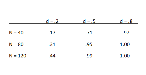
The analyses here focus on the handgrip paradigm because this paradigm has high power to detect moderate to strong effects because these studies measured handgrip strengths before and after the manipulation of will-power. Based on published studies, it is possible to estimate the retest correlation of handgrip performance (r ~ .8). Below are some a priori power analysis with common sample sizes and Cohen’s effect sizes of small, moderate, and large effect sizes.

HandgripPoewr

The power analysis shows that the pre-post design is very powerful to detect moderate to large effect sizes.   Even with a sample size of just 40 participants (20 per condition), power is 71%. If reporting bias and publication bias exclude 30% non-significant results from the evidence, observed power is inflated to 82%. The comparison of success rate (100%) and observed power (82%) leads to an estimated inflation rate of 18%) and an R-Index is 64% (82% – 18%). Thus a moderate effect size in studies with 40 or more participants is expected to produce an R-Index greater than 64%.

However, with typical sample sizes of less than 120 participants, the expected rate of significant results is less than 50%. With N = 80 and true power of 31%, the reporting of only significant results would boost the observed power to 64%. The inflation rate would be 30% and the R-Index would be 39%. In this case, the R-Index overestimates true power by 9%. Thus, an R-Index less than 50% suggests that the true effect size is small or that the null-hypothesis is true (importantly, the null-hypothesis refers to the effect in the handgrip-paradigm, not to the validity of the broader theory that it becomes more difficult to sustain effort over time).

R-Analysis

The meta-analysis included 18 effect sizes based on handgrip studies.   Two unpublished studies (Ns = 24, 37) were not included in this analysis.   Seeley & Gardner (2003)’s study was excluded because it failed to use a pre-post design, which could explain the non-significant result. The meta-analysis reported two effect sizes for this study. Thus, 4 effects were excluded and the analysis below is based on the remaining 14 studies.

All articles presented significant effects of will-power manipulations on handgrip performance. Bray et al. (2008) reported three tests; one was deemed not significant (p = .10), one marginally significant (.06), and one was significant at p = .05 (p = .01). The results from the lowest p-value were used. As a result, the success rate was 100%.

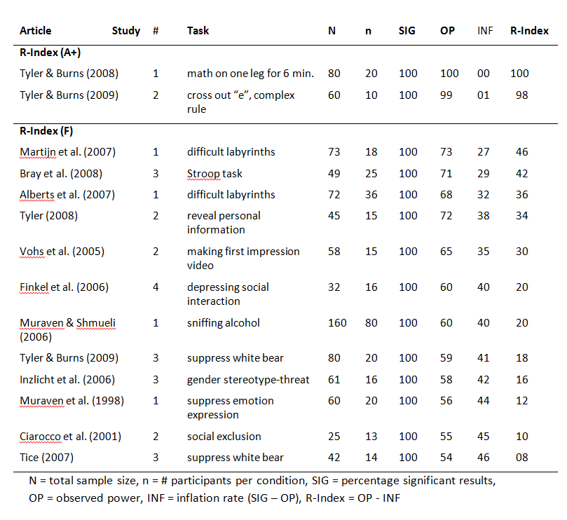
Median observed power was 63%. The inflation rate is 37% and the R-Index is 26%. An R-Index of 22% is consistent with a scenario in which the null-hypothesis is true and all reported findings are type-I errors. Thus, the R-Index supports Carter and McCullough’s (2014) conclusion that the existing evidence does not provide empirical support for the hypothesis that will-power manipulations lower performance on a measure of will-power.

The R-Index can also be used to examine whether a subset of studies provides some evidence for the will-power hypothesis, but that this evidence is masked by the noise generated by underpowered studies with small samples. Only 7 studies had samples with more than 50 participants. The R-Index for these studies remained low (20%). Only two studies had samples with 80 or more participants. The R-Index for these studies increased to 40%, which is still insufficient to estimate an unbiased effect size.

One reason for the weak results is that several studies used weak manipulations of will-power (e.g., sniffing alcohol vs. sniffing water in the control condition). The R-Index of individual studies shows two studies with strong results (R-Index > 80). One study used a physical manipulation (standing one leg). This manipulation may lower handgrip performance, but this effect may not reflect an influence on will-power. The other study used a mentally taxing (and boring) task that is not physically taxing as well, namely crossing out “e”s. This task seems promising for a replication study.

Power analysis with an effect size of d = .2 suggests that a serious empirical test of the will-power hypothesis requires a sample size of N = 300 (150 per cell) to have 80% power in a pre-post study of will-power.

 HandgripRindex


Conclusion

The R-Index of 14 will-power studies with the powerful pre-post handgrip paradigm confirms Carter and McCullough’s (2014) conclusion that a meta-analysis of will-power studies (Hagger Wood, & Chatzisarantis, 2010) provided an inflated estimate of the true effect size and that the existing studies provide no empirical support for the effect of will-power manipulations on a second effortful task. The existing studies have insufficient statistical power to distinguish a true null-effect from a small effect (d = .2). Power analysis suggest that future studies should focus on strong manipulations of will-power and use sample sizes of N = 300 participants.

Limitation

This analysis examined only a small set of studies in the meta-analysis that used handgrip performance as dependent variable. Other studies may show different results, but these studies often used a simple between-subject design with small samples. This paradigm has low power to detect even moderate effect sizes. It is therefore likely that the R-Index will also confirm Carter and McCullough’s (2014) conclusion.

The Replicability-Index (R-Index): Quantifying Research Integrity

ANNIVERSARY POST.  Slightly edited version of first R-Index Blog on December 1, 2014.

In a now infamous article, Bem (2011) produced 9 (out of 10) statistically significant results that appeared to show time-reversed causality.  Not surprisingly, subsequent studies failed to replicate this finding.  Although Bem never admitted it, it is likely that he used questionable research practices to produce his results. That is, he did not just run 10 studies and found 9 significant results. He may have dropped failed studies, deleted outliers, etc.  It is well-known among scientists (but not lay people) that researchers routinely use these questionable practices to produce results that advance their careers.  Think, doping for scientists.

I have developed a statistical index that tracks whether published results were obtained by conducting a series of studies with a good chance of producing a positive result (high statistical power) or whether researchers used questionable research practices.  The R-Index is a function of the observed power in a set of studies. More power means that results are likely to replicate in a replication attempt.  The second component of the R-index is the discrepancy between observed power and the rate of significant results. 100 studies with 80% power should produce, on average, 80% significant results. If observed power is 80% and the success rate is 100%, questionable research practices were used to obtain more significant results than the data justify.  In this case, the actual power is less than 80% because questionable research practices inflate observed power. The R-index subtracts the discrepancy (in this case 20% too many significant results) from observed power to adjust for the inflation.  For example, if observed power is 80% and success rate is 100%, the discrepancy is 20% and the R-index is 60%.

In a paper, I show that the R-index predicts success in empirical replication studies.

The R-index also sheds light on the recent controversy about failed replications in psychology (repligate) between replicators and “replihaters.”   Replicators sometimes imply that failed replications are to be expected because original studies used small samples with surprisingly large effects, possibly due to the use of questionable research practices. Replihaters counter that replicators are incompetent researchers who are motivated to produce failed studies.  The R-Index makes it possible to evaluate these claims objectively and scientifically.  It shows that the rampant use of questionable research practices in original studies makes it extremely likely that replication studies will fail.  Replihaters should take note that questionable research practices can be detected and that many failed replications are predicted by low statistical power in original articles.