Bayesian statistics is like all other statistics. A bunch of numbers are entered into a formula and the end result is another number.  The meaning of the number depends on the meaning of the numbers that enter the formula and the formulas that are used to transform them.

The input for a Bayesian inference is no different than the input for other statistical tests.  The input is information about an observed effect size and sampling error. The observed effect size is a function of the unknown population effect size and the unknown bias introduced by sampling error in a particular study.

Based on this information, frequentists compute p-values and some Bayesians compute a Bayes-Factor. The Bayes Factor expresses how compatible an observed test statistic (e.g., a t-value) is with one of two hypothesis. Typically, the observed t-value is compared to a distribution of t-values under the assumption that H0 is true (the population effect size is 0 and t-values are expected to follow a t-distribution centered over 0 and an alternative hypothesis. The alternative hypothesis assumes that the effect size is in a range from -infinity to infinity, which of course is true. To make this a workable alternative hypothesis, H1 assigns weights to these effect sizes. Effect sizes with bigger weights are assumed to be more likely than effect sizes with smaller weights. A weight of 0 would mean a priori that these effects cannot occur.

As Bayes-Factors depend on the weights attached to effect sizes, it is also important to realize that the support for H0 depends on the probability that the prior distribution was a reasonable distribution of probable effect sizes. It is always possible to get a Bayes-Factor that supports H0 with an unreasonable prior.  For example, an alternative hypothesis that assumes that an effect size is at least two standard deviations away from 0 will not be favored by data with an effect size of d = .5, and the BF will correctly favor H0 over this improbable alternative hypothesis.  This finding would not imply that the null-hypothesis is true. It only shows that the null-hypothesis is more compatible with the observed result than the alternative hypothesis. Thus, it is always necessary to specify and consider the nature of the alternative hypothesis to interpret Bayes-Factors.

Although the a priori probabilities of  H0 and H1 are both unknown, it is possible to test the plausibility of priors against actual data.  The reason is that observed effect sizes provide information about the plausible range of effect sizes. If most observed effect sizes are less than 1 standard deviation, it is not possible that most population effect sizes are greater than 1 standard deviation.  The reason is that sampling error is random and will lead to overestimation and underestimation of population effect sizes. Thus, if there were many population effect sizes greater than 1, one would also see many observed effect sizes greater than 1.

To my knowledge, proponents of Bayes-Factors have not attempted to validate their priors against actual data. This is especially problematic when priors are presented as defaults that require no further justification for a specification of H1.

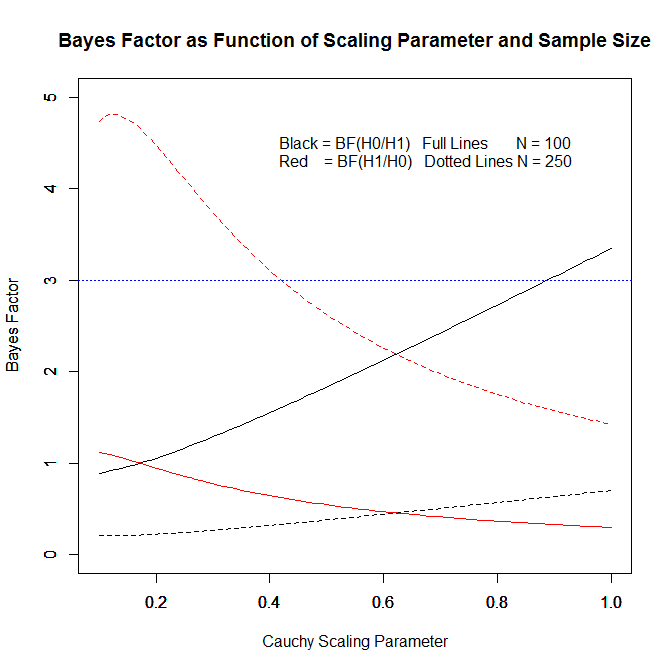
In this post, I focus on Wagenmakers’ prior because Wagenmaker has been a prominent advocate of Bayes-Factors as an alternative approach to conventional null-hypothesis-significance testing.  Wagenmakers’ prior is a Cauchy distribution with a scaling factor of 1.  This scaling factor implies a 50% probability that effect sizes are larger than 1 standard deviation.  This prior was used to argue that Bem’s (2011) evidence for PSI was weak. It has also been used in many other articles to suggest that the data favor the null-hypothesis.  These articles fail to point out that the interpretation of Bayes-Factors in favor of H0 is only valid for Wagenmakers’ prior. A different prior could have produced different conclusions.  Thus, it is necessary to examine whether Wagenmakers’ prior is a plausible prior for psychological science.

Wagenmakers’ Prior and Replicability

A prior distribution of effect sizes makes assumption about population effect sizes. In combination with information about sample size, it is possible to compute non-centrality parameters, which are equivalent to the population effect size divided by sampling error.  For each non-centrality parameter it is possible to estimate power as the area under the curve of the non-central t-distribution on the right side of the criterion value that corresponds to alpha, typically .05 (two-tailed).   The assumed typical power is simply the weighted average of the power values for each non-centrality parameters.

Replicability is not identical to power for a set of studies with heterogeneous non-centrality parameters because studies with higher power are more likely to become significant. Thus, the set of studies that achieved significance has higher average power as the original set of studies.

Aside from power, the distribution of observed test statistics is also informative. Unlikely power which is bound at 1, the distribution of test-statistics is unlimited. Thus, unreasonable assumptions about the distribution of effect sizes are visible in a distribution of test statistics that does not match distributions of tests statistics in actual studies.  One problem is that test-statistics are not directly comparable for different sample sizes or statistical tests because non-central distributions vary as a function of degrees of freedom and the test being used (e.g., chi-square vs. t-test).  To solve this problem, it is possible to convert all test statistics into z-scores so that they are on a common metric.  In a heterogeneous set of studies, the sign of the effect provides no useful information because signs only have to be consistent in tests of the same population effect size. As a result, it is necessary to use absolute z-scores. These absolute z-scores can be interpreted as the strength of evidence against the null-hypothesis.

I used a sample size of N = 80 and assumed a between subject design. In this case, sampling error is defined as 2/sqrt(80) = .224.  A sample size of N = 80 is the median sample size in Psychological Science. It is also the total sample size that would be obtained in a 2 x 2 ANOVA with n = 20 per cell.  Power and replicability estimates would increase for within-subject designs and for studies with larger N. Between subject designs with smaller N would yield lower estimates.

I simulated effect sizes in the range from 0 to 4 standard deviations.  Effect sizes of 4 or larger are extremely rare. Excluding these extreme values means that power estimates underestimate power slightly, but the effect is negligible because Wagenmakers’ prior assigns low probabilities (weights) to these effect sizes.

For each possible effect size in the range from 0 to 4 (using a resolution of d = .001)  I computed the non-centrality parameter as d/se.  With N = 80, these non-centrality parameters define a non-central t-distribution with 78 degrees of freedom.

I computed the implied power to achieve a significant result with alpha = .05 (two-tailed) with the formula

power = pt(ncp,N-2,qt(1-.025,N-2))

The formula returns the area under the curve on the right side of the criterion value that corresponds to a two-tailed test with p = .05.

The mean of these power values is the average power of studies if all effect sizes were equally likely.  The value is 89%. This implies that in the long run, a random sample of studies drawn from this population of effect sizes is expected to produce 89% significant results.

However, Wagenmakers’ prior assumes that smaller effect sizes are more likely than larger effect sizes. Thus, it is necessary to compute the weighted average of power using Wagenmakes’ prior distribution as weights.  The weights were obtained using the density of a Cauchy distribution with a scaling factor of 1 for each effect size.

wagenmakers.weights = dcauchy(es,0,1)

The weighted average power was computed as the sum of the weighted power estimates divided by the sum of weights.  The weighted average power is 69%.  This estimate implies that Wagenmakers’ prior assumes that 69% of statistical tests produce a significant result, when the null-hypothesis is false.

Replicability is always higher than power because the subset of studies that produce a significant result has higher average power than the the full set of studies. Replicabilty for a set of studies with heterogeneous power is the sum of the squared power of individual studies divided by the sum of power.

Replicability = sum(power^2) / sum(power)

The unweighted estimate of replicabilty is 96%.   To obtain the replicability for Wagenmakers’ prior, the same weighting scheme as for power can be used for replicability.

Wagenmakers.Replicability = sum(weights * power^2) / sum(weights*power)

The formula shows that Wagenmakers’ prior implies a replicabilty of 89%.  We see that the weighting scheme has relatively little effect on the estimate of replicability because many of the studies with small effect sizes are expected to produce a non-significant result, whereas the large effect sizes often have power close to 1, which implies that they wil be significant in the original study and the replication study.

The success rate of replication studies is difficult to estimate. Cohen estimated that typical studies in psychology have 50% power to detect a medium effect size, d = .5.  This would imply that the actual success rate would be lower because in an unknown percentage of studies the null-hypothesis is true.  However, replicability would be higher because studies with higher power are more likely to be significant.  Given this uncertainty, I used a scenario with 50% replicability.  That is an unbiased sample of studies taken from psychological journals would produce 50% successful replications in an exact replication study of the original studies.  The following computations show the implications of a 50% success rate in replication studies for the proportion of hypothesis tests where the null hypothesis is true, p(H0).

The percentage of true null-hypothesis is a function of the success rate in replication study, weighted average power, and weighted replicability.

p(H0) = (weighted.average.power * (weighted.replicability – success.rate)) / (success.rate*.05 – success.rate*weighted.average.power – .05^2 + weighted.average.power*weighted.replicability)

To produce a success rate of 50% in replication studies with Wagenmakers’ prior when H1 is true (89% replicability), the percentage of true null-hypothesis has to be 92%.

The high percentage of true null-hypothesis (92%) also has implications for the implied false-positive rate (i.e., the percentage of significant results that are true null-hypothesis.

False Positive Rate =  (Type.1.Error *.05)  / (Type.1.Error * .05 +
(1-Type.1.Error) * Weighted.Average.Power)
For every 100 studies, there are 92 true null-hypothesis that produce 92*.05 = 4.6 false positive results. For the remaining 8 studies with a true effect, there are 8 * .67 = 5.4 true discoveries.  The false positive rate is 4.6 / (4.6 + 5.4) = 46%.  This means Wagenmakers prior assumes that a success rate of 50% in replication studies implies that nearly 50% of studies that replicate successfully are false-positives results that would not replicate in future replication studies.

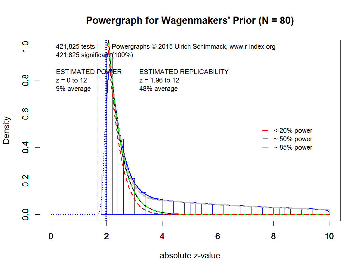
Aside from these analytically derived predictions about power and replicability, Wagenmakers’ prior also makes predictions about the distribution of observed evidence in individual studies. As observed scores are influenced by sampling error, I used simulations to illustrate the effect of Wagenmakers’ prior on observed test statistics.

For the simulation I converted the non-central t-values into non-central z-scores and simulated sampling error with a standard normal distribution.  The simulation included 92% true null-hypotheses and 8% true H1 based on Wagenmaker’s prior.  As published results suffer from publication bias, I simulated publication bias by selecting only observed absolute z-scores greater than 1.96, which corresponds to the p < .05 (two-tailed) significance criterion.  The simulated data were submitted to a powergraph analysis that estimates power and replicability based on the distribution of absolute z-scores.

Figure 1 shows the results.   First, the estimation method slightly underestimated the actual replicability of 50% by 2 percentage points.  Despite this slight estimation error, the Figure accurately illustrates the implications of Wagenmakers’ prior for observed distributions of absolute z-scores.  The density function shows a steep decrease in the range of z-scores between 2 and 3, and a gentle slope for z-scores greater than 4 to 10 (values greater than 10 are not shown).

Powergraphs provide some information about the composition of the total density by dividing the total density into densities for power less than 20%, 20-50%, 50% to 85% and more than 85%. The red line (power < 20%) mostly determines the shape of the total density function for z-scores from 2 to 2.5, and most the remaining density is due to studies with more than 85% power starting with z-scores around 4.   Studies with power in the range between 20% and 85% contribute very little to the total density. Thus, the plot correctly reveals that Wagenmakers’ prior assumes that the roughly 50% average replicability is mostly due to studies with very low power (< 20%) and studies with very high power (> 85%).

Validation Study 1: Michael Nujiten’s Statcheck Data

There are a number of datasets that can be used to evaluate Wagenmakers’ prior. The first dataset is based on an automatic extraction of test statistics from psychological journals. I used Michael Nuijten’s dataset to ensure that I did not cheery-pick data and to allow other researchers to reproduce the results.

The main problem with automatically extracted test statistics is that the dataset does not distinguish between  theoretically important test statistics and other statistics, such as significance tests of manipulation checks.  It is also not possible to distinguish between between-subject and within-subject designs.  As a result, replicability estimates for this dataset will be higher than the simulation based on a between-subject design.

Figure 2 shows all of the data, but only significant z-scores (z > 1.96) are used to estimate replicability and power. The most striking difference between Figure 1 and Figure 2 is the shape of the total density on the right side of the significance criterion.  In Figure 2 the slope is shallower. The difference is visible in the decomposition of the total density into densities for different power bands.  In Figure 1 most of the total density was accounted for by studies with less than 20% power and studies with more than 85% power.  In Figure 2, studies with power in the range between 20% and 85% account for the majority of studies with z-scores greater than 2.5 up to z-scores of 4.5.

The difference between Figure 1 and Figure 2 has direct implications for the interpretation of Bayes-Factors with t-values that correspond to z-scores in the range of just significant results. Given Wagenmakers’ prior, z-scores in this range mostly represent false-positive results. However, the real dataset suggests that some of these z-scores are the result of underpowered studies and publication bias. That is, in these studies the null-hypothesis is false, but the significant result will not replicate because these studies have low power.

Validation Study 2:  Open Science Collective Articles (Original Results)

The second dataset is based on the Open Science Collective (OSC) replication project.  The project aimed to replicate studies published in three major psychology journals in the year 2008.  The final number of articles that were selected for replication was 99. The project replicated one study per article, but articles often contained multiple studies.  I computed absolute z-scores for theoretically important tests from all studies of these 99 articles.  This analysis produced 294 test statistics that could be converted into absolute z-scores.

Figure 3 shows clear evidence of publication bias.  No sampling distribution can produce the steep increase in tests around the critical value for significance. This selection is not an artifact of my extraction, but an actual feature of published results in psychological journals (Sterling, 1959).

Given the small number of studies, the figure also contains bootstrapped 95% confidence intervals.  The 95% CI for the power estimate shows that the sample is too small to estimate power for all studies, including studies in the proverbial file drawer, based on the subset of studies that were published. However, the replicability estimate of 49% has a reasonably tight confidence interval ranging from 45% to 66%.

The shape of the density distribution in Figure 3 differs from the distribution in Figure 2 in two ways. Initially the slop is steeper in Figure 3, and there is less density in the tail with high z-scores.  Both aspects contribute to the lower estimate of replicability in Figure 3, suggesting that replicabilty of focal hypothesis tests is lower than replicabilty for all statistical tests.

Comparing Figure 3 and Figure 1 shows again that the powergraph based on Wagenmakers’ prior differs from the powergraph for real data. In this case, the discrepancy is even more notable because focal hypothesis tests rarely produce large z-scores (z > 6).

Validation Study 3:  Open Science Collective Articles (Replication Results)

At present, the only data that are somewhat representative of psychological research (at least of social and cognitive psychology) and that do not suffer from publication bias are the results from the replication studies of the OSC replication project.  Out of 97 significant results in original studies, 36 studies (37%) produced that produced a significant result in the original studies produced a significant result in the replication study.  After eliminating some replication studies (e.g., sample of replication study was considerably smaller), 88 studies remained.

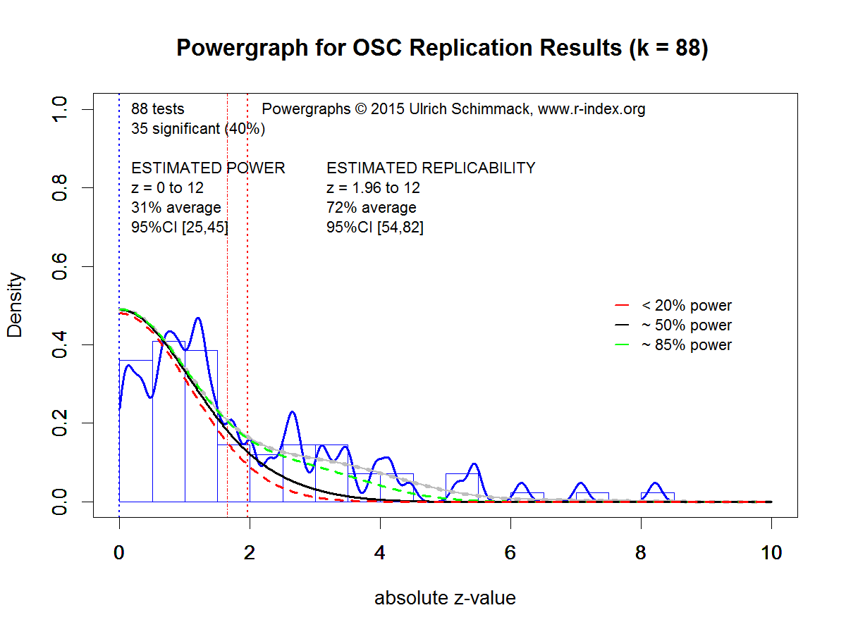
Figure 4 shows the powergraph for the 88 studies. As there is no publication bias, estimates of power and replicability are based on non-significant and significant results.  Although the sample size is smaller, the estimate of power has a reasonably narrow confidence interval because the estimate includes non-significant results. Estimated power is only 31%. The 95% confidence interval includes the actual success rate of 40%, which shows that there is no evidence of publication bias.

A visual comparison of Figure 1 and Figure 4 shows again that real data diverge from the predicted pattern by Wagenmakers’ prior.  Real data show a greater contribution of power in the range between 20% and 85% to the total density, and large z-scores (z > 6) are relatively rare in real data.

Conclusion

Statisticians have noted that it is good practice to examine the assumptions underlying statistical tests. This blog post critically examines the assumptions underlying the use of Bayes-Factors with Wagenmakers’ prior.  The main finding is that Wagenmaker’s prior makes unreasonable assumptions about power, replicability, and the distribution of observed test-statistics with or without publication bias. The main problem from Wagenmakers’ prior is that it predicts too many statistical results with strong evidence against the null-hypothesis (z > 5, or the 5 sigma rule in physics).  To achieve reasonable predictions for success rates without publication bias (~50%), Wagenmakers’ prior has to assume that over 90% of statistical tests conducted in psychology test false hypothesis (i.e., predict an effect when H0 is true), and that the false-positive rate is close to 50%.

Implications

Bayesian statisticians have pointed out for a long time that the choice of a prior influences Bayes-Factors (Kass, 1993, p. 554).  It is therefore useful to carefully examine priors to assess the effect of priors on Bayesian inferences. Unreasonable priors will lead to unreasonable inferences.  This is also true for Wagenmakers’ prior.

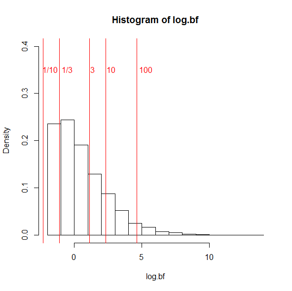
The problem of using Bayes-Factors with Wagenmakers’ prior to test the null-hypothesis is apparent in a realistic scenario that assumes a moderate population effect size of d = .5 and a sample size of N = 80 in a between subject design. This study has a non-central t of 2.24 and 60% power to produce a significant result with p < .05, two-tailed.   I used R to simulate 10,000 test-statistics using the non-central t-distribution and then computed Bayes-Factors with Wagenmakers’ prior.

Figure 5 shows a histogram of log(BF). The log is being used because BF are ratios and have very skewed distributions.  The histogram shows that BF never favor the null-hypothesis with a BF of 10 in favor of H0 (1/10 in the histogram).  The reason is that even with Wagenmakers’ prior a sample size of N = 80 is too small to provide strong support for the null-hypothesis.  However, 21% of observed test statistics produce a Bayes-Factor less than 1/3, which is sometimes used as sufficient evidence to claim that the data support the null-hypothesis.  This means that the test has a 21% error rate to provide evidence for the null-hypothesis when the null-hypothesis is false.  A 21% error rate is 4 times larger than the 5% error rate in null-hypothesis significance testing. It is not clear why researchers should replace a statistical method with a 5% error rate for a false discovery of an effect with a 20% error rate of false discoveries of null effects.

Another 48% of the results produce Bayes-Factors that are considered inconclusive. This leaves 31% of results that favor H1 with a Bayes-Factor greater than 3, and only 17% of results produce a Bayes-Factor greater than 10.   This implies that even with the low standard of a BF > 3, the test has only 31% power to provide evidence for an effect that is present.

These results are not wrong because they correctly express the support that the observed data provide for H0 and H1.  The problem only occurs when the specification of H1 is ignored. Given Wagenmakers prior, it is much more likely that a t-value of 1 stems from the sampling distribution of H0 than from the sampling distribution of H1.  However, studies with 50% power when an effect is present are also much more likely to produce t-values of 1 than t-values of 6 or larger.   Thus, a different prior that is more consistent with the actual power of studies in psychology would produce different Bayes-Factors and reduce the percentage of false discoveries of null effects.  Thus, researchers who think Wagenmakers’ prior is not a realistic prior for their research domain should use a more suitable prior for their research domain.

Counterarguments

Wagenmakers’ has ignored previous criticisms of his prior.  It is therefore not clear what counterarguments he would make.  Below, I raise some potential counterarguments that might be used to defend the use of Wagenmakers’ prior.

One counterargument could be that the prior is not very important because the influence of priors on Bayes-Factors decreases as sample sizes increase.  However, this argument ignores the fact that Bayes-Factors are often used to draw inferences from small samples. In addition, Kass (1993) pointed out that “a simple asymptotic analysis shows that even in large samples Bayes factors remain sensitive to the choice of prior” (p. 555).

Another counterargument could be that a bias in favor of H0 is desirable because it keeps the rate of false-positives low. The problem with this argument is that Bayesian statistics does not provide information about false-positive rates.  Moreover, the cost for reducing false-positives is an increase in the rate of false negatives; that is, either inconclusive results or false evidence for H0 when an effect is actually present.  Finally, the choice of the correct prior will minimize the overall amount of errors.  Thus, it should be desirable for researchers interested in Bayesian statistics to find the most appropriate priors in order to minimize the rate of false inferences.

A third counterargument could be that Wagenmakers’ prior expresses a state of maximum uncertainty, which can be considered a reasonable default when no data are available.  If one considers each study as a unique study, a default prior of maximum uncertainty would be a reasonable starting point.  In contrast, it may be questionable to treat a new study as a randomly drawn study from a sample of studies with different population effect sizes.  However, Wagenmakers’ prior does not express a state of maximum uncertainty and makes assumptions about the probability of observing very large effect sizes.  It does so without any justification for this expectation.  It therefore seems more reasonable to construct priors that are consistent with past studies and to evaluate priors against actual results of studies.

A fourth counterargument is that Bayes-Factors are superior because they can provide evidence for the null-hypothesis and the alternative hypothesis.  However, this is not correct. Bayes-Factors only provide relative support for the null-hypothesis relative to a specific alternative hypothesis.  Researchers who are interested in testing the null-hypothesis can do so using parameter estimation with confidence or credibility intervals. If the interval falls within a specified region around zero, it is possible to affirm the null-hypothesis with a specified level of certainty that is determined by the precision of the study to estimate the population effect size.  Thus, it is not necessary to use Bayes-Factors to test the null-hypothesis.

In conclusion, Bayesian statistics and other statistics are not right or wrong. They combine assumptions and data to draw inferences.  Untrustworthy data and wrong assumptions can lead to false conclusions.  It is therefore important to test the integrity of data (e.g., presence of publication bias) and to examine assumptions.  The uncritical use of Bayes-Factors with default assumptions is not good scientific practice and can lead to false conclusions just like the uncritical use of p-values can lead to false conclusions.