Correction (2026-07-14)
The original post claimed that violations of the normality assumption biases standard random effects estimates. That finding was based on a coding error in the simulation program. The revised post shows the results for simulations with normal distributed effect sizes for H1 and mixtures of H0 and H1. In these simulations only estimates of the weight-function selection model (weightr package) are biased when the unimodal normal distribution assumption is violated.
Introduction
The main purpose of meta-analysis is to combine the results of quantitative studies. The simplest form averages the effect-size estimates of studies. The average is a better estimate of the population effect size because it draws on the combined sample size of the individual studies, and larger samples have less sampling error. A more sophisticated version takes each study’s sampling error into account, weighting studies with larger samples more heavily than those with smaller samples. This weighted average approximates the estimate one would obtain by pooling the raw data, under the assumption that all studies estimate the same effect.
These so-called fixed-effect meta-analyses assume that the samples are all drawn from the same population and that studies used interchangeable procedures, so that they all estimate a single population effect size. This assumption is defensible for a few phenomena grounded in basic sensory or cognitive architecture. Weber’s law, for instance — that the just-noticeable difference between two stimuli is a roughly constant proportion of their magnitude — reflects a property of sensory transduction and varies little across procedures and individuals. But such near-constants are the exception. Most effects in psychology vary with situational and personality factors, within and across cultures. This variation adds real differences in the true effect sizes across studies, over and above sampling error.
In recognition of this true variation, statisticians developed random-effects models (DerSimonian & Laird, 1986). To model the variation in population effect sizes, it is necessary to select a model that describes the unobserved variation in population effect sizes. From a statistical perspective, the easiest model assumes that population effect sizes have a normal distribution. The symmetry of this assumption implies that the estimate obtained from a set of studies is an unbiased estimate of the true average because positive and negative deviations from the average population effect size cancel each other out, just like random sampling errors cancel each other out.
Distribution Assumptions
From a theoretical perspective, it is unlikely that population effect sizes are normally distributed, particularly when the mean effect is small relative to the between-study heterogeneity. The reason is that effects are typically coded so that positive values are consistent with a directional theoretical prediction (e.g., conflicting colors produce slower responses in the Stroop task). While the size of the effect may vary across studies, it is often implausible that the true effect in some studies would be reversed (that conflicting colors would genuinely speed responses). A normal distribution, however, has support over the entire range of effect sizes and therefore always assigns some probability to negative true effects — an implication that is difficult to justify for a directionally predicted effect. When the mean is small relative to the heterogeneity, a normal distribution implies that a non-trivial proportion of true effects are negative, which is often theoretically implausible.
In practice, however, when heterogeneity is small, violations of the normality assumption have small and often negligible effects on meta-analytic estimates of the average effect (Hedges & Vevea, 1996). This helps explain why widely used random-effects models share the assumption that population effect sizes are normally distributed, including standard random-effects meta-analysis (DerSimonian & Laird, 1986) as implemented in commonly used software (Viechtbauer, 2010), selection-model approaches (Vevea & Hedges, 1995; Vevea & Woods, 2005), and the random-effects components of Bayesian model-averaging methods (Bartoš et al., 2023; Maier et al., 2023).
Necessary and Unnecessary Assumptions
It is useful to distinguish between necessary and unnecessary assumptions. All statistical methods require some assumptions to reduce the complex information in data to an interpretable statistic. However, not all assumptions of a model are necessary. In general, models with fewer unnecessary assumptions are preferable because they are robust to violations of these unnecessary assumptions by design. For example, the Pearson correlation coefficient assumes normal distribution of the two variables, whereas rank-order correlations do not. This makes rank-order correlations robust to violations of the normal distribution assumption and it is common practice to prefer rank-order correlations when variables’ distributions are not normal.
In meta-analyses, the assumption that population effect sizes are normally distributed is an unnecessary assumption. The idea of estimating the distribution of effects without assuming a parametric form is not new. Laird (1978) and Lindsay (1983) showed that the mixing distribution in a mixture model can be estimated nonparametrically by maximum likelihood, and that the resulting estimate takes the form of a discrete distribution on a finite set of support points. This provided, in principle, a fully flexible way to model heterogeneity without assuming normality. In practice, however, fitting these models was computationally demanding at the time.
Advances in optimization and computing have since removed these hurdles. Efficient algorithms for estimating mixture models — including modern convex-optimization methods (Koenker & Mizera, 2014; Kim et al., 2020) — now make it possible to fit flexible mixtures quickly and reliably. These developments led to the widespread adoption of nonparametric and empirical-Bayes mixture models in fields that analyze large numbers of effects, most notably genomics (Efron, 2010; Stephens, 2017), where the goal is to characterize the distribution of effects across thousands of tests and to identify which are likely to be real. Similar approaches have been applied in astronomy, education, and other areas that deal with many parallel estimates.
Heterogeneity of Population Effect Sizes
Meta-analysis, however, did not adopt these models, and continued to rely on the normal random-effects model. One reason is that the goal of most meta-analyses has been to estimate a single average effect, for which the shape of the effect-size distribution is largely irrelevant. The additional information provided by a flexible mixture — the structure of the heterogeneity itself — was not part of the question being asked.
This has changed with growing recognition of the distinction between direct and conceptual replication (Zwaan et al., 2018). Experimental psychologists rarely repeat a procedure exactly. Instead, they typically vary paradigms across studies in the belief that this is good scientific practice — probing moderators, boundary conditions, and the generalizability of an effect. As a result, the studies combined in a meta-analysis often estimate genuinely different population effects, and meta-analyses of such conceptual replications frequently show high estimates of heterogeneity (van Erp et al., 2017). In these cases the average effect size is of relatively minor interest, because it merely centers a wide distribution of different population effect sizes — an average across paradigm variants that no single study actually instantiates. The scientifically interesting question is not the average, but how and why the effects differ.
Mixture Models
Mixture models have another advantage over random effects models for meta-analysis. In standard meta-analytic models the population distribution of effect sizes is characterized by the mean and standard deviation of a normal distribution. Importantly, this information is removed from the observed data. It is therefore not possible to use this information to make sense of the heterogeneity in the observed effect size estimates in the data. A large effect size in the data may correspond to a small population effect size because it was inflated by sampling error and vice versa. This explains why heterogeneity often plays a minor role in the interpretation of meta-analyses. Heterogeneity exists, but it cannot be explained.
In contrast, mixture models combined with statistical tools that correct for regression to the mean make it possible to obtain estimates of the population effect size of individual studies. Often these effect size estimates for single studies have large uncertainty (wide confidence intervals), but they can be averaged to identify subgroups of studies with large effect sizes. This makes it possible to explore the heterogeneity in observed studies.
Simulation Study
To demonstrate the capabilities and advantages of mixture models over traditional random-effects models, I conducted a simulation study. To isolate the effect of the distributional assumption, the simulation used unbiased data (no publication selection). This removes selection as a confound and allows inclusion of the adaptive-shrinkage mixture model ash (Stephens, 2017), which was developed for genomics and assumes complete, unselected data. The other two models — the weight-function selection model (Vevea & Woods, 2005) and z-curve — model publication bias but reduce to unbiased estimation when no selection is present.
Z-curve is a meta-analytic mixture model (Brunner & Schimmack, 2020; Bartoš & Schimmack, 2022). Version 1 used the noncentrality parameters (ncp) of significant results to estimate the expected replication rate for direct replication studies. Version 2 used the ncp distribution across all studies to estimate the expected discovery rate. Version 3 adds an empirical-Bayes function that estimates population effect sizes by multiplying ncp estimates by their corresponding sampling errors, recovering effects from the latent distribution of noncentrality parameters.
The simulation used fixed sample sizes across studies, which ensures that mixture models fit in the effect-size metric and in the ncp metric produce identical results. Each condition contained k = 1,000 studies; the large k yields small sampling error in the estimates, making systematic biases more visible. The design crossed 4 means and 4 standard deviations of the population effect-size distribution with 4 proportions of true null hypotheses, producing 64 conditions. The population effect sizes when H1 is true were drawn from a normal distribution. However, mixing true H0 and H1 produces non-normal, bimodal distributions. This violates the distribution assumption of standard meta-analytic methods and could produce biased estimates.
zcurve3.0/SimpleMix_All_Normal_ZC_ASHR_VW_RMA.R at main · UlrichSchimmack/zcurve3.0
Results
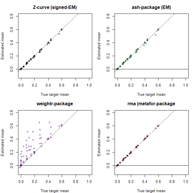
These results for the mixture models (z-curve, ash) are not surprising. The models make no distribution assumptions and estimates of the mean closely match the simulated true values (z-curve RMSE = .009; ash RMSE = .010). The weight-function selection model had worse fit (RMSE = .138), but the random effects model fit as well as the mixture models (RMA RMSE = .003).
The results for the estimate of heterogeneity (tau) showed that all models estimated heterogeneity well, (z-curve RMSE = .018, ash RMSE = .027, weightr RMSE = .030, RMA RMSE = .013).
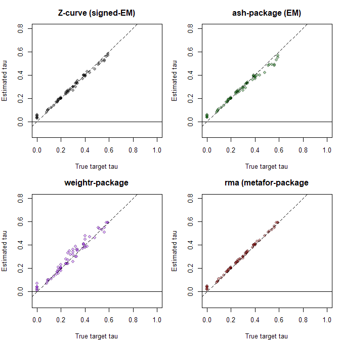
The present results show that the random effects model is robust to violations of the normality assumption even when heterogeneity is large and distributions are bimodal. The same cannot be said for the selection model with a normal assumption (weightr). Here the weight parameters to model selection bias can be biased to fit a normal distribution to non-normal observed data. The main implication is that it is possible to improve the performance of selection models by avoiding the normality assumption and modeling the distribution of population effect sizes with a flexible mixture model.
Implications
The present simulation showed that the random-effects model estimates the mean effect well when data are unbiased, even when its distributional assumptions are violated. This is consistent with a substantial prior literature. Simulation studies have repeatedly found that the pooled mean from the normal random-effects model is robust to non-normal random-effects distributions, including skewed and mixture distributions (Yamaguchi et al., 2017; Rubio-Aparicio et al., 2023; Baur et al., 2025). The robustness follows from the estimator itself: the pooled mean is an inverse-variance weighted average, which is consistent for the population mean regardless of the shape of the effect distribution. Large numbers of studies further protect against non-normality (Rubio-Aparicio et al., 2023), and with k = 1,000 the present simulation is in this favorable regime.
Where the normality assumption does matter is not the mean but the characterization of the distribution around it. The same literature finds that non-normality degrades the coverage of confidence and prediction intervals far more than it biases the mean (Baur et al., 2025), and that a symmetric normal model produces a wrongly symmetric prediction interval and a misleading heterogeneity summary when the true distribution is skewed (Yamaguchi et al., 2017). The recognized advantage of flexible mixture and semi-parametric models is therefore not lower bias on the mean but their ability to reveal latent structure — clusters and subgroups of studies — that the mean and a single heterogeneity parameter discard (Baur et al., 2025).
These are real but secondary limitations. The more fundamental problem is one that no distributional flexibility can address: the random-effects model, and the adaptive-shrinkage mixture model (ash) alike, assume that the observed studies are an unbiased sample of the population. In many literatures this assumption is untenable. In psychology, studies with significant results are far more likely to be published; the proportion of significant results often exceeds 90% (Sterling et al., 1995). Such publication bias inflates effect-size estimates, and correcting for it requires modeling the selection process — something neither the random-effects model nor ash attempts. A flexible distribution alone is not enough; what is needed is a model that combines distributional flexibility with a model of selection.
Z-curve occupies this niche: it combines a selection model, which corrects for publication bias, with a flexible mixture model, which captures heterogeneity without a distributional assumption. This is why z-curve outperforms weight-function models when studies are both heterogeneous and affected by publication bias (Schimmack, 2026).
References:
Bartoš, F., Maier, M., Wagenmakers, E.-J., Doucouliagos, H., & Stanley, T. D. (2023). Robust Bayesian meta-analysis: Model-averaging across complementary publication bias adjustment methods. Research Synthesis Methods, 14(1), 99–116.
Böhning, D. (2000). Computer-assisted analysis of mixtures and applications: Meta-analysis, disease mapping and others. Chapman & Hall/CRC.
DerSimonian, R., & Laird, N. (1986). Meta-analysis in clinical trials. Controlled Clinical Trials, 7(3), 177–188.
Hedges, L. V., & Vevea, J. L. (1996). Estimating effect size under publication bias: Small sample properties and robustness of a random effects selection model. Journal of Educational and Behavioral Statistics, 21(4), 299–332.
Laird, N. (1978). Nonparametric maximum likelihood estimation of a mixing distribution. Journal of the American Statistical Association, 73(364), 805–811.
Lindsay, B. G. (1983). The geometry of mixture likelihoods: A general theory. The Annals of Statistics, 11(1), 86–94.
Maier, M., Bartoš, F., & Wagenmakers, E.-J. (2023). Robust Bayesian meta-analysis: Addressing publication bias with model-averaging. Psychological Methods, 28(1), 107–122.
Stephens, M. (2017). False discovery rates: A new deal. Biostatistics, 18(2), 275–294.
Vevea, J. L., & Hedges, L. V. (1995). A general linear model for estimating effect size in the presence of publication bias. Psychometrika, 60(3), 419–435.
Vevea, J. L., & Woods, C. M. (2005). Publication bias in research synthesis: Sensitivity analysis using a priori weight functions. Psychological Methods, 10(4), 428–443.
Viechtbauer, W. (2010). Conducting meta-analyses in R with the metafor package. Journal of Statistical Software, 36(3), 1–48.
Efron, B. (2010). Large-scale inference: Empirical Bayes methods for estimation, testing, and prediction. Cambridge University Press.
Kim, Y., Carbonetto, P., Stephens, M., & Koenker, R. (2020). A fast algorithm for maximum likelihood estimation of mixture proportions using sequential quadratic programming. Journal of Computational and Graphical Statistics, 29(2), 261–273.
Koenker, R., & Mizera, I. (2014). Convex optimization, shape constraints, compound decisions, and empirical Bayes rules. Journal of the American Statistical Association, 109(506), 674–685.
Laird, N. (1978). Nonparametric maximum likelihood estimation of a mixing distribution. Journal of the American Statistical Association, 73(364), 805–811.
Lindsay, B. G. (1983). The geometry of mixture likelihoods: A general theory. The Annals of Statistics, 11(1), 86–94.