I am all in favor of open science and a critic of closed pre-publication peer-review. The downside of open communication is that there is no quality control and internet searches will amplify misinformation. This is the case with Erik van Zwet’s critique of z-curve. Even though I addressed his criticisms in the comment section, search engines – like humans – do not scroll to the end and process all information. I have even addressed concerns about z-curve.2.0 by improving z-curve 3.0 to handle edge cases like the one used by van Zwet to cast doubt about z-curves performance in general. In science, facts trump visibility Z-curve.has been validated with many simulations across a wide range of scenarios and works well even with just 50 significant z-values. For more information, check out the Replication Index blog or the FAQ about z-curve page.
The bias in the Bing (AI) summary is evident when we compare it to Google search summary. Still makes a false claim about assumptions based on Erik van Zwet’s blog bost, but also avoids the dismissal of a method based on a single edge case that was easy to address and is no longer of concern in the new z-curve.3.0. In short, don’t trust the first generic response of AI. Use AI to probe arguments.
Bartoš, F., & Schimmack, U. (2022). Z-curve 2.0: Estimating replication rates and discovery rates. Meta-Psychology, 6, Article e0000130. https://doi.org/10.15626/MP.2022.2981
Brunner, J., & Schimmack, U. (2020). Estimating population mean power under conditions of heterogeneity and selection for significance. Meta- Psychology. MP.2018.874, https://doi.org/10.15626/MP.2018.874
van Zwet, E., Gelman, A., Greenland, S., Imbens, G., Schwab, S., & Goodman, S. N. (2024). A New Look at P Values for Randomized Clinical Trials. NEJM evidence, 3(1), EVIDoa2300003. https://doi.org/10.1056/EVIDoa2300003
The Story of Two Z-Curve Models
Erik van Zwet recently posted a critique of the z-curve method on Andrew Gelman’s blog.
Meaningful discussion of the severity and scope of this critique was difficult in that forum, so I address the issue more carefully here.
van Zwet identified a situation in which z-curve can overestimate the Expected Discovery Rate (EDR) when it is inferred from the distribution of statistically significant z-values. Specifically, when the distribution of significant results is driven primarily by studies with high power, the observed distribution contains little information about the distribution of nonsignificant results. If those nonsignificant results are not reported and z-curve is nevertheless used to infer them from the significant results alone, the method can underestimate the number of missing nonsignificant studies and, as a consequence, overestimate the Expected Discovery Rate (EDR).
This is a genuine limitation, but it is a conditional and diagnosable one. Crucially, the problematic scenarios are directly observable in the data. Problematic data have an increasing or flat slope of the significant z-value distribution and a mode well above the significance threshold. In such cases, z-curve does not silently fail; it signals that inference about missing studies is weak and that EDR estimates should not be trusted.
This is rarely a problem in psychology, where most studies have low power, the mode is at the significance criterion, and the slope decreases, often steeply. This pattern implies a large set of non-significant results and z-curve provides good estimates in these scenarios. It is difficult to estimate distributions of unobserved data, leading to wide confidence intervals around these estimates. However, there is no fixed number of studies that are needed. The relevant question is whether the confidence intervals are informative enough to support meaningful conclusions.
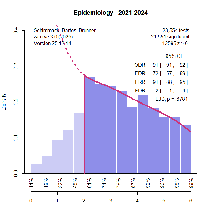
One of the most powerful set of studies that I have actually seen comes from epidemiology, where studies often have large samples to estimate effect sizes precisely. In these studies, power to reject the null hypothesis is actually not really important, but the data serve as a good example of a set of studies with high power, rather than low power as in psychology.
However, even this example shows a decreasing slope and a mode at significance criterion. Fitting z-curve to these data still suggests some selection bias and no underestimation of reported non-significant results. This illustrates how extreme van Zwet’s scenario must be to produce the increasing-slope pattern that undermines EDR estimation.
What about van Zwet’s Z-Curve Method?
It is also noteworthy that van Zwet does not compare our z-curve method (Bartos & Schimmack, 2022; Brunner & Bartos, 2020) to his own z-curve method that was used to analyze z-values from clinical trials (van Zwet et al., 2024).
The article fits a model to the distribution of absolute z-values (ignoring whether results show a benefit or harm to patients). The key differences between the two approaches are that (a) van Zwet et al.’s model uses all z-values and assumes (implicitly) that there is no selection bias, and (b) that true effect sizes are never zero and errors can only be sign errors. Based on these assumptions, the article concludes that no more than 2% of clinical trials produce a result that falsely rejects a true hypothesis. For example, a statistically significant result could be treated as an error only if the true effect has the opposite sign (e.g., the true effect increases smoking, but a significant result is used to claim it reduced smoking).
The advantage of this method is that it is not necessary to estimate the EDR from the distribution of only significant results, but it does so only by assuming that publication bias does not exist. In this case, we can just count the observed non-significant and significant results and use the observed discovery rate to estimate average power and the false positive risk.
The trade-off is clear. z-curve attempts to address selection bias and sometimes lacks sufficient information to do so reliably; van Zwet’s approach achieves stable estimates by assuming the problem away. The former risks imprecision when information is weak; the latter risks bias when its core assumption is violated.
In the example from epidemiology, there is evidence of some publication bias and omission of non-significant results. Using van Zwet’s model would be inappropriate because it would overestimate the true discovery rate. The focus on sign errors alone is also questionable and should be clearly stated as a strong assumption. It implies that significant results in the right direction are not errors, even if effect sizes are close to zero. For example, a significant result that suggests it extends life is considered a true finding, even if the effect size is one day.
False positive rates do not fully solve that problem, but false positive rates that include zero as a hypothetical value for the population effect size are higher and treat small effects close to zero as errors rather than treating half of them as correct rejections of the null hypothesis. For example, an intervention that decreases smoking by 1% of all smokers is not really different from one that increases it by 1%, but a focus on signs treats only the latter one as an error.
In short, van Zwet’s critique identifies a boundary condition for z-curve, not a general failure. At the same time, his own method rests on a stronger and untested assumption—no selection bias—whose violation would invalidate its conclusions entirely. No method is perfect and using a single scenario to imply that a method is always wrong is not a valid argument against any method. By the same logic, van Zwet’s own method could be declared “useless” whenever selection bias exists, which is precisely the point: all methods have scope conditions.
Using proper logic, we suggest that all methods work when assumptions are met. The main point is to test whether they are met or not. We clarified that z-curve estimation of the EDR assumes that enough low powered studies produced significant results to influence the distribution of significant results. If the slope of significant results is not decreasing, this assumption does not hold and z-curve should not be used to estimate the EDR. Similarly, users of van Zwets first method should first test whether selection bias is present and not use it when it does. They should also examine whether they think a proportion of studies could have tested practically true null hypotheses and not use the method when this is a concern.
Finally, the blog post responds to Gelman’s polemic about our z-curve method and earlier work by Jager and Leek (2014), by noting that Gelman’s critic of other methods exist in parallel to his own work (at least co-authorship) that also modeled distribution of z-values to make claims about power and the risk of false inferences. The assumption of this model that selection bias does not exist is peculiar, given Gelman’s typical writing about low power and the negative effects of selection for significance. A more constructive discussion would apply the same critical standards to all methods—including one’s own.
“What I’d like to say is that it is OK to criticize a paper, even [if, typo in original] it isn’t horrible.” (Gelman, 2023)
In this spirit, I would like to criticize Loken and Gelman’s confusing article about the interpretation of effect sizes in studies with small samples and selection for significance. They compare random measurement error to a backpack and the outcome of a study to running speed. Common sense suggests that the same individual under identical conditions would run faster without a backpack than with a backpack. The same outcome is also suggested by psychometric theories that suggest random measurement error attenuates population effect sizes, which would make it harder to demonstrate significance and produce, on average, weaker effect sizes.
The key point of Loken and Gelman’s article is to suggest that this intuition fails under some conditions. “Should we assume that if statistical significance is achieved in the presence of measurement error, the associated effects would have been stronger without noise? We caution against the fallacy”
To support their clam that common sense is a fallacy under certain conditions, they present the results of a simple simulation study. After some concerns about their conclusions were raised, Loken and Gelman shared the actual code of their simulation study. In this blog post, I share the code with annotations and reproduce their results. I also show that their results are based on selecting for significance only for the measure with random measurement error (with a backpack) and not for the measure without a backpack (no random measurement error). Reversing the selection shows that selection for significance without measurement error produces stronger effect sizes even more often than selection for significance with a backpack. Thus, it is not a fallacy to assume that we would all run faster without a backpack holding all other factors equal. However, a runner with a heavy backpack and tailwinds might run faster than a runner without a backpack facing strong headwinds. While this is true, the influence of wind on performance makes it difficult to see the influence of the backpack. Under identical conditions backpacks slow people down and random measurement error attenuates effects.
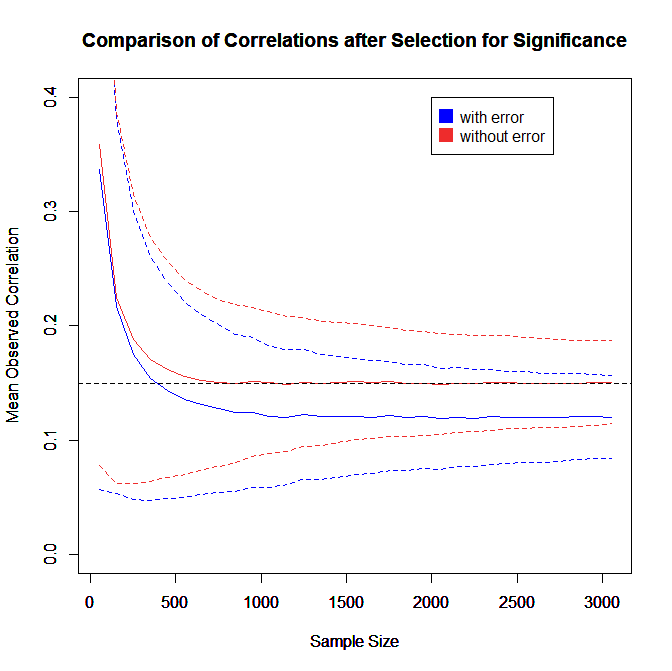
Loken and Gelman’s presentation of the results may explain why some readers, including us, misinterpreted their results to imply that selection bias and random measurement error may interaction in some complex way to produce even more inflated estimates of the true correlation. We added some lines of code to their simulation to compute the average correlations after selection for significance separately for the measure without error and the measure with error. This way, both measures benefit equally from selection bias. The plot also provides more direct evidence about the amount of bias that is introduced by selection bias and random measurement error. In addition, the plot shows the average 95% confidence intervals around the estimated correlation coefficients.
The plot shows that for large samples (N > 1,000), the measure without error always produces the expected true correlation of r = .15, whereas the measure with error always produces the expected attenuated correlation of r = .15 * .80 = .12. As sample sizes get smaller, the effect of selection bias becomes apparent. For the measure without error, the observed effect sizes are now inflated. For the measure with error, selection bias corrects for the inflation and the two biases cancel each other out to produce more accurate estimates of the true effect size than with the measure without error. For sample sizes below N = 400, however, both measures produce inflated estimates and in really small samples the attenuation effect due to unreliability is overwhelmed by selection bias. However, while the difference due to unreliability is negligible and approaches zero, it is clear that random measurement error combined with selection bias never produces even stronger estimates than the measure without error. Thus, it remains true that we should expect a measure without random measurement error to produce stronger correlations than a measure with random error. This fundamental principle of psychometrics, however, does not warrant the conclusion that an observed statistically significant correlation in small samples underestimates the true correlation coefficient because the correlation may have been inflated by selection for significance.
The plot also shows how researchers can avoid misinterpretation of inflated effect size estimates in small samples. In small samples, confidence intervals are wide. Figure 2 shows that the confidence interval around inflated effect size estimates in small samples is so wide that it includes the true correlation of r = .15. The width of the confidence interval in small samples make it clear that the study provided no meaningful information about the size of an effect. This does not mean the results are useless. After all, the results correctly show that the relationship between the variables is positive rather than negative. For the purpose of effect size estimation it is necessary to conduct meta-analysis and to include studies with significant and non-significant results. Furthermore, meta-analysis need to test for the presence of selection bias and correct for it when it is present.
P.S. If somebody claims that they ran a marathon in 2 hours with a heavy backpack, they may not be lying. They may just not tell you all of the information. We often fill in the blanks and that is where things can go wrong. If the backpack were a jet pack and the person was using it to fly for some of the race, we would no longer be surprised by the amazing feat. Similarly, if somebody tells you that they got a correlation of r = .8 in a sample of N = 8 with a measure that has only 20% reliable variance, you should not be surprised if they tell you that they got this result after picking 1 out of 20 studies because selection for significance will produce strong correlations in small samples even if there is no correlation at all. Once they tell you that they tried many times to get the one significant result, it is obvious that the next study is unlikely to replicate a significant result.
Sometimes You Can Be Faster With a Heavy Backpack
Annotated Original Code
### This is the final code used for the simulation studies posted by Andrew Gelman on his blog
### Comments are highlighted with my initials #US#
# First just the original two plots, high power N = 3000, low power N = 50, true slope = .15
r <- .15
sims<-array(0,c(1000,4))
xerror <- 0.5
yerror<-0.5
for (i in 1:1000) {
x <- rnorm(50,0,1)
y <- r*x + rnorm(50,0,1)
#US# this is a sloppy way to simulate a correlation of r = .15
#US# The proper code is r*x + rnorm(50,0,1)*sqrt(1-r^2)
#US# However, with the specific value of r = .15, the difference is trivial
#US# However, however, it raises some concerns about expertise
xx<-lm(y~x)
sims[i,1]<-summary(xx)$coefficients[2,1]
x<-x + rnorm(50,0,xerror)
y<-y + rnorm(50,0,yerror)
xx<-lm(y~x)
sims[i,2]<-summary(xx)$coefficients[2,1]
x <- rnorm(3000,0,1)
y <- r*x + rnorm(3000,0,1)
xx<-lm(y~x)
sims[i,3]<-summary(xx)$coefficients[2,1]
x<-x + rnorm(3000,0,xerror)
y<-y + rnorm(3000,0,yerror)
xx<-lm(y~x)
sims[i,4]<-summary(xx)$coefficients[2,1]
}
plot(sims[,2] ~ sims[,1],ylab=”Observed with added error”,xlab=”Ideal Study”)
abline(0,1,col=”red”)
plot(sims[,4] ~ sims[,3],ylab=”Observed with added error”,xlab=”Ideal Study”)
abline(0,1,col=”red”)
#US# There is no major issue with graphs 1 and 2.
#US# They merely show that high sampling error produces large uncertainty in the estimates.
#US# The small attenuation effect of r = .15 vs. r = 12 is overwhelmed by sampling error
#US# The real issue is the simulation of selection for significance in the third graph
# third graph
# run 2000 regressions at points between N = 50 and N = 3050
r <- .15
propor <-numeric(31)
powers<-seq(50,3050,100)
#US# These lines of code are added to illustrate the biased selection for significane
propor.reversed.selection <-numeric(31)
mean.sig.cor.without.error <- numeric(31) # mean correlation for the measure without error when t > 2
mean.sig.cor.with.error <- numeric(31) # mean correlation for the measure with error when t > 2
#US# It is sloppy to refer to sample sizes as powers.
#US# In between subject studies, the power to produce a true positive result
#US# is a function of the population correlation and the sample size
#US# With population correlations fixed at r = .15 or r = .12, sample size is the
#US# only variable that influences power
#US# However, power varies from alpha to 1 and it would be interesting to compare the
#US# power of studies with r = .15 and r = .12 to produce a significant result.
#US# The claim that “one would always run faster without a backback”
#US# could be interpreted as a claim that it is always easier to obtain a
#US# significant result without measurement error, r = .15, than with measurement error, r = .12
#US# This claim can be tested with Loken and Gelman’s simulation by computing
#US# the percentage of significant results obtained without and with measurement error
#US# Loken and Golman do not show this comparison of power.
#US# The reason might be the confusion of sample size with power.
#US# While sample sizes are held constant, power varies as a function of the population correlations
#US# without, r = .15, and with, r = .12, measurement error.
xerror<-0.5
yerror<-0.5
j = 1
i = 1
for (j in 1:31) {
sims<-array(0,c(1000,4))
for (i in 1:1000) {
x <- rnorm(powers[j],0,1)
y <- r*x + rnorm(powers[j],0,1)
#US# the same sloppy simulation of population correlations as before
xx<-lm(y~x)
sims[i,1:2]<-summary(xx)$coefficients[2,1:2]
x<-x + rnorm(powers[j],0,xerror)
y<-y + rnorm(powers[j],0,yerror)
xx<-lm(y~x)
sims[i,3:4]<-summary(xx)$coefficients[2,1:2]
}
#US# The code is the same as before, it just adds variation in sample sizes
#US# The crucial aspect to understand figure 3 is the following code that
#US# compares the results for the paired outcomes without and with measurement error
#US# Carlos Ungil (https://ch.linkedin.com/in/ungil) pointed out on Gelman’s blog #US# that there is another sloppy mistake in the simulation code that does not alter the results #US# The code compares absolute t-values (coefficient/sampling error), while the article #US# talks about inflated effect size estimates. However, while the sampling error variation #US# creates some variability, the pattern remains the same. #US# For sake of reproducibility I kept the comparison of t-values.
# find significant observations (t test > 2) and then check proportion
temp<-sims[abs(sims[,3]/sims[,4])> 2,]
#US# the use of t > 2 is sloppy and unnecessary.
#US# summary(lm) gives the exact p-values that could be used to select for significance
#US# summary(xx)[2,4] < .05
#US# However, this does not make a substantial difference
#US# The crucial part of this code is that it uses the outcomes of the simulation
#US# with random measurement error to select for significance
#US# As outcomes are paired, this means that the code sometimes selects outcomes
#US# in which sampling error produces significance with random measurement error