Tag Archives: Questionable Research Practices

Questionable Research Practices: Definition, Detection, and Recommendations for Better Practices

How Power Analysis Could Have Prevented the Sad Story of Dr. Förster

[further information can be found in a follow up blog]

Background

In 2011, Dr. Förster published an article in Journal of Experimental Psychology: General. The article reported 12 studies and each study reported several hypothesis tests. The abstract reports that “In all experiments, global/local processing in 1 modality shifted to global/local processing in the other modality”.

For a while this article was just another article that reported a large number of studies that all worked and neither reviewers nor the editor who accepted the manuscript for publication found anything wrong with the reported results.

In 2012, an anonymous letter voiced suspicion that Jens Forster violated rules of scientific misconduct. The allegation led to an investigation, but as of today (January 1, 2015) there is no satisfactory account of what happened. Jens Förster maintains that he is innocent (5b. Brief von Jens Förster vom 10. September 2014) and blames the accusations about scientific misconduct on a climate of hypervigilance after the discovery of scientific misconduct by another social psychologist.

The Accusation

The accusation is based on an unusual statistical pattern in three publications. The 3 articles reported 40 experiments with 2284 participants, that is an average sample size of N = 57 participants in each experiment. The 40 experiments all had a between-subject design with three groups: one group received a manipulation design to increase scores on the dependent variable. A second group received the opposite manipulation to decrease scores on the dependent variable. And a third group served as a control condition with the expectation that the average of the group would fall in the middle of the two other groups. To demonstrate that both manipulations have an effect, both experimental groups have to show significant differences from the control group.

The accuser noticed that the reported means were unusually close to a linear trend. This means that the two experimental conditions showed markedly symmetrical deviations from the control group. For example, if one manipulation increased scores on the dependent variables by half a standard deviation (d = +.5), the other manipulation decreased scores on the dependent variable by half a standard deviation (d = -.5). Such a symmetrical pattern can be expected when the two manipulations are equally strong AND WHEN SAMPLE SIZES ARE LARGE ENOUGH TO MINIMIZE RANDOM SAMPLING ERROR. However, the sample sizes were small (n = 20 per condition, N = 60 per study). These sample sizes are not unusual and social psychologists often use n = 20 per condition to plan studies. However, these sample sizes have low power to produce consistent results across a large number of studies.

The accuser computed the statistical probability of obtaining the reported linear trend. The probability of obtaining the picture-perfect pattern of means by chance alone was incredibly small.

Based on this finding, the Dutch National Board for Research Integrity (LOWI) started an investigation of the causes for this unlikely finding. An English translation of the final report was published on retraction watch. An important question was whether the reported results could have been obtained by means of questionable research practices or whether the statistical pattern can only be explained by data manipulation. The English translation of the final report includes two relevant passages.

According to one statistical expert “QRP cannot be excluded, which in the opinion of the expert is a common, if not “prevalent” practice, in this field of science.” This would mean that Dr. Förster acted in accordance with scientific practices and that his behavior would not constitute scientific misconduct.

In response to this assessment the Complainant “extensively counters the expert’s claim that the unlikely patterns in the experiments can be explained by QRP.” This led to the decision that scientific misconduct occurred.

Four QRPs were considered.

  1. Improper rounding of p-values. This QRP can only be used rarely when p-values happen to be close to .05. It is correct that this QRP cannot produce highly unusual patterns in a series of replication studies. It can also be easily checked by computing exact p-values from reported test statistics.
  2. Selecting dependent variables from a set of dependent variables. The articles in question reported several experiments that used the same dependent variable. Thus, this QRP cannot explain the unusual pattern in the data.
  3. Collecting additional research data after an initial research finding revealed a non-significant result. This description of an QRP is ambiguous. Presumably it refers to optional stopping. That is, when the data trend in the right direction to continue data collection with repeated checking of p-values and stopping when the p-value is significant. This practices lead to random variation in sample sizes. However, studies in the reported articles all have more or less 20 participants per condition. Thus, optional stopping can be ruled out. However, if a condition with 20 participants does not produce a significant result, it could simply be discarded, and another condition with 20 participants could be run. With a false-positive rate of 5%, this procedure will eventually yield the desired outcome while holding sample size constant. It seems implausible that Dr. Förster conducted 20 studies to obtain a single significant result. Thus, it is even more plausible that the effect is actually there, but that studies with n = 20 per condition have low power. If power were just 30%, the effect would appear in every third study significantly, and only 60 participants were used to produce significant results in one out of three studies. The report provides insufficient information to rule out this QRP, although it is well-known that excluding failed studies is a common practice in all sciences.
  4. Selectively and secretly deleting data of participants (i.e., outliers) to arrive at significant results. The report provides no explanation how this QRP can be ruled out as an explanation. Simmons, Nelson, and Simonsohn (2011) demonstrated that conducting a study with 37 participants and then deleting data from 17 participants can contribute to a significant result when the null-hypothesis is true. However, if an actual effect is present, fewer participants need to be deleted to obtain a significant result. If the original sample size is large enough, it is always possible to delete cases to end up with a significant result. Of course, at some point selective and secretive deletion of observation is just data fabrication. Rather than making up data, actual data from participants are deleted to end up with the desired pattern of results. However, without information about the true effect size, it is difficult to determine whether an effect was present and just embellished (see Fisher’s analysis of Mendel’s famous genetics studies) or whether the null-hypothesis is true.

The English translation of the report does not contain any statements about questionable research practices from Dr. Förster. In an email communication on January 2, 2014, Dr. Förster revealed that he in fact ran multiple studies, some of which did not produce significant results, and that he only reported his best studies. He also mentioned that he openly admitted to this common practice to the commission. The English translation of the final report does not mention this fact. Thus, it remains an open question whether QRPs could have produced the unusual linearity in Dr. Förster’s studies.

A New Perspective: The Curse of Low Powered Studies

One unresolved question is why Dr. Förster would manipulate data to produce a linear pattern of means that he did not even mention in his articles. (Discover magazine).

One plausible answer is that the linear pattern is the by-product of questionable research practices to claim that two experimental groups with opposite manipulations are both significantly different from a control group. To support this claim, the articles always report contrasts of the experimental conditions and the control condition (see Table below). ForsterTable

In Table 1 the results of these critical tests are reported with subscripts next to the reported means. As the direction of the effect is theoretically determined, a one-tailed test was used. The null-hypothesis was rejected when p < .05.

Table 1 reports 9 comparisons of global processing conditions and control groups and 9 comparisons of local processing conditions with a control group; a total of 18 critical significance tests. All studies had approximately 20 participants per condition. The average effect size across the 18 studies is d = .71 (median d = .68).   An a priori power analysis with d = .7, N = 40, and significance criterion .05 (one-tailed) gives a power estimate of 69%.

An alternative approach is to compute observed power for each study and to use median observed power (MOP) as an estimate of true power. This approach is more appropriate when effect sizes vary across studies. In this case, it leads to the same conclusion, MOP = 67.

The MOP estimate of power implies that a set of 100 tests is expected to produce 67 significant results and 33 non-significant results. For a set of 18 tests, the expected values are 12.4 significant results and 5.6 non-significant results.

The actual success rate in Table 1 should be easy to infer from Table 1, but there are some inaccuracies in the subscripts. For example, Study 1a shows no significant difference between means of 38 and 31 (d = .60, but it shows a significant difference between means 31 and 27 (d = .33). Most likely the subscript for the control condition should be c not a.

Based on the reported means and standard deviations, the actual success rate with N = 40 and p < .05 (one-tailed) is 83% (15 significant and 3 non-significant results).

The actual success rate (83%) is higher than one would expect based on MOP (67%). This inflation in the success rate suggests that the reported results are biased in favor of significant results (the reasons for this bias are irrelevant for the following discussion, but it could be produced by not reporting studies with non-significant results, which would be consistent with Dr. Förster’s account ).

The R-Index was developed to correct for this bias. The R-Index subtracts the inflation rate (83% – 67% = 16%) from MOP. For the data in Table 1, the R-Index is 51% (67% – 16%).

Given the use of a between-subject design and approximately equal sample sizes in all studies, the inflation in power can be used to estimate inflation of effect sizes. A study with N = 40 and p < .05 (one-tailed) has 50% power when d = .50.

Thus, one interpretation of the results in Table 1 is that the true effect sizes of the manipulation is d = .5, that 9 out of 18 tests should have produced a significant contrast at p < .05 (one-tailed) and that questionable research practices were used to increase the success rate from 50% to 83% (15 vs. 9 successes).

The use of questionable research practices would also explain unusual linearity in the data. Questionable research practices will increase or omit effect sizes that are insufficient to produce a significant result. With a sample size of N = 40, an effect size of d = .5 is insufficient to produce a significant result, d = .5, se = 32, t(38) = 1.58, p = .06 (one-tailed). Random sampling error that works against the hypothesis can only produce non-significant results that have to be dropped or moved upwards using questionable methods. Random error that favors the hypothesis will inflate the effect size and start producing significant results. However, random error is normally distributed around the true effect size and is more likely to produce results that are just significant (d = .8) than to produce results that are very significant (d = 1.5). Thus, the reported effect sizes will be clustered more closely around the median inflated effect size than one would expect based on an unbiased sample of effect sizes.

The clustering of effect sizes will happen for the positive effects in the global processing condition and for the negative effects in the local processing condition. As a result, the pattern of all three means will be more linear than an unbiased set of studies would predict. In a large set of studies, this bias will produce a very low p-value.

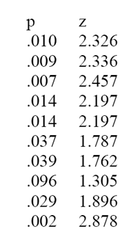
One way to test this hypothesis is to examine the variability in the reported results. The Test of Insufficient Variance (TIVA) was developed for this purpose. TIVA first converts p-values into z-scores. The variance of z-scores is known to be 1. Thus, a representative sample of z-scores should have a variance of 1, but questionable research practices lead to a reduction in variance. The probability that a set of z-scores is a representative set of z-scores can be computed with a chi-square test and chi-square is a function of the ratio of the expected and observed variance and the number of studies. For the set of studies in Table 1, the variance in z-scores is .33. The chi-square value is 54. With 17 degrees of freedom, the p-value is 0.00000917 and the odds of this event occurring by chance are 1 out of 109,056 times.

Conclusion

Previous discussions about abnormal linearity in Dr. Förster’s studies have failed to provide a satisfactory answer. An anonymous accuser claimed that the data were fabricated or manipulated, which the author vehemently denies. This blog proposes a plausible explanation of what could have [edited January 19, 2015] happened. Dr. Förster may have conducted more studies than were reported and included only studies with significant results in his articles. Slight variation in sample sizes suggests that he may also have removed a few outliers selectively to compensate for low power. Importantly, neither of these practices would imply scientific misconduct. The conclusion of the commission that scientific misconduct occurred rests on the assumption that QRPs cannot explain the unusual linearity of means, but this blog points out how selective reporting of positive results may have inadvertently produced this linear pattern of means. Thus, the present analysis support the conclusion by an independent statistical expert mentioned in the LOWI report: “QRP cannot be excluded, which in the opinion of the expert is a common, if not “prevalent” practice, in this field of science.”

How Unusual is an R-Index of 51?

The R-Index for the 18 statistical tests reported in Table 1 is 51% and TIVA confirms that the reported p-values have insufficient variance. Thus, it is highly probable that questionable research practices contributed to the results and in a personal communication Dr. Förster confirmed that additional studies with non-significant results exist. However, in response to further inquiries [see follow up blog] Dr. Förster denied having used QRPs that could explain the linearity in his data.

Nevertheless, an R-Index of 51% is not unusual and has been explained with the use of QRPs.  For example, the R-Index for a set of studies by Roy Baumeister was 49%, . and Roy Baumeister stated that QRPs were used to obtain significant results.

“We did run multiple studies, some of which did not work, and some of which worked better than others. You may think that not reporting the less successful studies is wrong, but that is how the field works.”

Sadly, it is quite common to find an R-Index of 50% or lower for prominent publications in social psychology. This is not surprising because questionable research practices were considered good practices until recently. Even at present, it is not clear whether these practices constitute scientific misconduct (see discussion in Dialogue, Newsletter of the Society for Personality and Social Psychology).

How to Avoid Similar Sad Stories in the Future

One way to avoid accusations of scientific misconduct is to conduct a priori power analyses and to conduct only studies with a realistic chance to produce a significant result when the hypothesis is correct. When random error is small, true patterns in data can emerge without the help of QRPs.

Another important lesson from this story is to reduce the number of statistical tests as much as possible. Table 1 reported 18 statistical tests with the aim to demonstrate significance in each test. Even with a liberal criterion of .1 (one-tailed), it is highly unlikely that so many significant tests will produce positive results. Thus, a non-significant result is likely to emerge and researchers should think ahead of time how they would deal with non-significant results.

For the data in Table 1, Dr. Förster could have reported the means of 9 small studies without significance tests and conduct significance tests only once for the pattern in all 9 studies. With a total sample size of 360 participants (9 * 40), this test would have 90% power even if the effect size is only d = .35. With 90% power, the total power to obtain significant differences from the control condition for both manipulations would be 81%. Thus, the same amount of resources that were used for the controversial findings could have been used to conduct a powerful empirical test of theoretical predictions without the need to hide inconclusive, non-significant results in studies with low power.

Jacob Cohen has been trying to teach psychologists the importance of statistical power for decades and psychologists stubbornly ignored his valuable contribution to research methodology until he died in 1998. Methodologists have been mystified by the refusal of psychologists to increase power in their studies (Maxwell, 2004).

One explanation is that small samples provided a huge incentive. A non-significant result can be discarded with little cost of resources, whereas a significant result can be published and have the additional benefit of an inflated effect size, which allows boosting the importance of published results.

The R-Index was developed to balance the incentive structure towards studies with high power. A low R-Index reveals that a researcher is reporting biased results that will be difficult to replicate by other researchers. The R-Index reveals this inconvenient truth and lowers excitement about incredible results that are indeed incredible. The R-Index can also be used by researchers to control their own excitement about results that are mostly due to sampling error and to curb the excitement of eager research assistants that may be motivated to bias results to please a professor.

Curbed excitement does not mean that the R-Index makes science less exciting. Indeed, it will be exciting when social psychologists start reporting credible results about social behavior that boost a high R-Index because for a true scientist nothing is more exciting than the truth.

The Test of Insufficient Variance (TIVA): A New Tool for the Detection of Questionable Research Practices

Citation. Schimmack, U. (2015). The Test of Insufficient
Variance (TIVA): A new tool for the detection of questionable research practices. Retrieved from http:// replicationindex.wordpress.com/2015/01/01/tiva

Updated 2025/08/20
I never submitted this work for peer-review, but the method has been reviewed in a peer-reviewed article and compared to other bias detection tools. Like many other tests, it does not work well when heterogeneity in effect sizes or sample sizes (or both) produces heterogeneity in power, but it did really well when all studies tested similar effect sizes which is often the case when they are small or zero.

Renkewitz, F., & Keiner, M. (2019). How to detect publication bias in psychological research: A comparative evaluation of six statistical methods. Zeitschrift für Psychologie, 227(4), 261–279. https://doi.org/10.1027/2151-2604/a000386

The Test of Insufficient Variance

It has been known for decades that published results tend to be biased (Sterling, 1959). For most of the past decades this inconvenient truth has been ignored. In the past years, there have been many suggestions and initiatives to increase the replicability of reported scientific findings (Asendorpf et al., 2013). One approach is to examine published research results for evidence of questionable research practices (see Schimmack, 2014, for a discussion of existing tests). This blog post introduces a new test of bias in reported research findings, namely the Test of Insufficient Variance (TIVA).

TIVA is applicable to any set of studies that used null-hypothesis testing to conclude that empirical data provide support for an empirical relationship and reported a significance test (p-values).

Rosenthal (1978) developed a method to combine results of several independent studies by converting p-values into z-scores. This conversion uses the well-known fact that p-values correspond to the area under the curve of a normal distribution. Rosenthal did not discuss the relation between these z-scores and power analysis. Z-scores are observed scores that should follow a normal distribution around the non-centrality parameter that determines how much power a study has to produce a significant result. In the Figure, the non-centrality parameter is 2.2. This value is slightly above a z-score of 1.96, which corresponds to a two-tailed p-value of .05. A study with a non-centrality parameter of 2.2 has 60% power.  In specific studies, the observed z-scores vary as a function of random sampling error. The standardized normal distribution predicts the distribution of observed z-scores. As observed z-scores follow the standard normal distribution, the variance of an unbiased set of z-scores is 1.  The Figure on top illustrates this with the nine purple lines, which are nine randomly generated z-scores with a variance of 1.

In a real data set the variance can be greater than 1 for two reasons. First, if the nine studies are exact replication studies with different sample sizes, larger samples will have a higher non-centrality parameter than smaller samples. This variance in the true non-centrality variances adds to the variance produced by random sampling error. Second, a set of studies that are not exact replication studies can have variance greater than 1 because the true effect sizes can vary across studies. Again, the variance in true effect sizes produces variance in the true non-centrality parameters that add to the variance produced by random sampling error.  In short, the variance is 1 in exact replication studies that also hold the sample size constant. When sample sizes and true effect sizes vary, the variance in observed z-scores is greater than 1. Thus, an unbiased set of z-scores should have a minimum variance of 1.

If the variance in z-scores is less than 1, it suggests that the set of z-scores is biased. One simple reason for insufficient variance is publication bias. If power is 50% and the non-centrality parameter matches the significance criterion of 1.96, 50% of studies that were conducted would not be significant. If these studies are omitted from the set of studies, variance decreases from 1 to .36. Another reason for insufficient variance is that researchers do not report non-significant results or used questionable research practices to inflate effect size estimates. The effect is that variance in observed z-scores is restricted.  Thus, insufficient variance in observed z-scores reveals that the reported results are biased and provide an inflated estimate of effect size and replicability.

In small sets of studies, insufficient variance may be due to chance alone. It is possible to quantify how lucky a researcher was to obtain significant results with insufficient variance. This probability is a function of two parameters: (a) the ratio of the observed variance (OV) in a sample over the population variance (i.e., 1), and (b) the number of z-scores minus 1 as the degrees of freedom (k -1).

The product of these two parameters follows a chi-square distribution with k-1 degrees of freedom.

Formula 1: Chi-square = OV * (k – 1) with k-1 degrees of freedom.

Example 1:

Bem (2011) published controversial evidence that appear to demonstrate precognition. Subsequent studies failed to replicate these results (Galak et al.,, 2012) and other bias tests show evidence that the reported results are biased Schimmack (2012). For this reason, Bem’s article provides a good test case for TIVA.

Bem_p_ZThe article reported results of 10 studies with 9 z-scores being significant at p < .05 (one-tailed). The observed variance in the 10 z-scores is 0.19. Using Formula 1, the chi-square value is chi^2 (df = 9) = 1.75. Importantly, chi-square tests are usually used to test whether variance is greater than expected by chance (right tail of the distribution). The reason is that variance is not expected to be less than the variance expected by chance because it is typically assumed that a set of data is unbiased. To obtain a probability of insufficient variance, it is necessary to test the left-tail of the chi-square distribution.  The corresponding p-value for chi^2 (df = 9) = 1.75 is p = .005. Thus, there is only a 1 out of 200 probability that a random set of 10 studies would produce a variance as low as Var = .19.

This outcome cannot be attributed to publication bias because all studies were published in a single article. Thus, TIVA supports the hypothesis that the insufficient variance in Bem’s z-scores is the result of questionable research methods and that the reported effect size of d = .2 is inflated. The presence of bias does not imply that the true effect size is 0, but it does strongly suggest that the true effect size is smaller than the average effect size in a set of studies with insufficient variance.

Example 2:  

Vohs et al. (2006) published a series of studies that he results of nine experiments in which participants were reminded of money. The results appeared to show that “money brings about a self-sufficient orientation.” Francis and colleagues suggested that the reported results are too good to be true. An R-Index analysis showed an R-Index of 21, which is consistent with a model in which the null-hypothesis is true and only significant results are reported.

Because Vohs et al. (2006) conducted multiple tests in some studies, the median p-value was used for conversion into z-scores. The p-values and z-scores for the nine studies are reported in Table 2. The Figure on top of this blog illustrates the distribution of the 9 z-scores relative to the expected standard normal distribution.

Table 2

Study                    p             z          

Study 1                .026       2.23
Study 2                .050       1.96
Study 3                .046       1.99
Study 4                .039       2.06
Study 5                .021       2.99
Study 6                .040       2.06
Study 7                .026       2.23
Study 8                .023       2.28
Study 9                .006       2.73
                                                           

The variance of the 9 z-scores is .054. This is even lower than the variance in Bem’s studies. The chi^2 test shows that this variance is significantly less than expected from an unbiased set of studies, chi^2 (df = 8) = 1.12, p = .003. An unusual event like this would occur in only 1 out of 381 studies by chance alone.

In conclusion, insufficient variance in z-scores shows that it is extremely likely that the reported results overestimate the true effect size and replicability of the reported studies. This confirms earlier claims that the results in this article are too good to be true (Francis et al., 2014). However, TIVA is more powerful than the Test of Excessive Significance and can provide more conclusive evidence that questionable research practices were used to inflate effect sizes and the rate of significant results in a set of studies.

Conclusion

TIVA can be used to examine whether a set of published p-values was obtained with the help of questionable research practices. When p-values are converted into z-scores, the variance of z-scores should be greater or equal to 1. Insufficient variance suggests that questionable research practices were used to avoid publishing non-significant results; this includes simply not reporting failed studies.

At least within psychology, these questionable research practices are used frequently to compensate for low statistical power and they are not considered scientific misconduct by governing bodies of psychological science (APA, APS, SPSP). Thus, the present results do not imply scientific misconduct by Bem or Vohs, just like the use of performance enhancing drugs in sports is not illegal unless a drug is put on an anti-doping list. However, jut because a drug is not officially banned, it does not mean that the use of a drug has no negative effects on a sport and its reputation.

One limitation of TIVA is that it requires a set of studies and that variance in small sets of studies can vary considerably just by chance. Another limitation is that TIVA is not very sensitive when there is substantial heterogeneity in true non-centrality parameters. In this case, the true variance in z-scores can mask insufficient variance in random sampling error. For this reason, TIVA is best used in conjunction with other bias tests. Despite these limitations, the present examples illustrate that TIVA can be a powerful tool in the detection of questionable research practices.  Hopefully, this demonstration will lead to changes in the way researchers view questionable research practices and how the scientific community evaluates results that are statistically improbable. With rejection rates at top journals of 80% or more, one would hope that in the future editors will favor articles that report results from studies with high statistical power that obtain significant results that are caused by the predicted effect.

Roy Baumeister’s R-Index

“We did run multiple studies, some of which did not work, and some of which worked better than others. You may think that not reporting the less successful studies is wrong, but that is how the field works.” (Roy Baumeister, personal email communication)

The R-Index can be used to evaluate the replicability of a set of statistical results. It can be used to evaluate the statistical research integrity of journals, articles on a specific topic (meta-analysis), and researchers. Just like the H-Index has become a popular metric of research excellence, the R-Index of individual researchers can be used to evaluate the replicability of their findings.

I chose Roy Baumeister as an example for several reasons. First, the R-Index is based on my earlier work on the incredibility-index (Schimmack, 2012). In this article, I demonstrated how power analysis can be used to reveal that researchers used questionable research practices to produce statistically significant results. I illustrated this approach with two articles. One article published 10 experiments that appeared to demonstrate time-reversed causality. Independent replication studies failed to replicate this incredible finding. The Incredibility-Index predicted this failure. The second article was a study on glucose consumption and will-power with Roy Baumeister as the senior author. The Incredibility-Index showed that the statistical results reported in this article were even less credible than the time-travel studies in Bem’s (2011) article.

Not surprisingly, Roy Baumeister was a reviewer of the incredibility article. During the review process, Roy Baumeister explained why his article reported more significant results than one would expect on the basis of the statistical power of these studies.

“My paper with Gailliot et al. (2007) is used as an illustration here. Of course, I am quite familiar with the process and history of that one. We initially submitted it with more studies, some of which had weaker results. The editor said to delete those. He wanted the paper shorter so as not to use up a lot of journal space with mediocre results. It worked: the resulting paper is shorter and stronger. Does that count as magic? The studies deleted at the editor’s request are not the only story. I am pretty sure there were other studies that did not work. Let us suppose that our hypotheses were correct and that our research was impeccable. Then several of our studies would have failed, simply given the realities of low power and random fluctuations. Is anyone surprised that those studies were not included in the draft we submitted for publication? If we had included them, certainly the editor and reviewers would have criticized them and formed a more negative impression of the paper. Let us suppose that they still thought the work deserved publication (after all, as I said, we are assuming here that the research was impeccable and the hypotheses correct). Do you think the editor would have wanted to include those studies in the published version?”

To my knowledge this is one of the few frank acknowledgements that questionable research practices (i.e., excluding evidence that does not support an author’s theory) contributed to the picture-perfect results in a published article. It is therefore instructive to examine the R-Index of a researcher who openly acknowledged that the reported results are a biased selection of the empirical evidence.

A tricky issue in any statistical analysis is the sampling of studies. In this case it would be possible to conduct the analysis on the full set of articles published by Roy Baumeister. However, for my analysis I selected a sample. To ensure that the sample is unbiased, I chose a sampling strategy that makes a priori sense and does not involve random sampling because I have control over the random generator. My sampling strategy was to focus on the Top 10 most cited original research articles.

To evaluate the R-Index, it is instructive to keep the following scenarios in mind.

  1. The null-hypothesis is true and a researcher uses questionable research practices to obtain just significant results (p = .049999). The observed power for this set of studies is 50%, but all statistical results are significant, 100% success rate. The success rate is inflated by 50%. The R-Index is observed power minus inflation rate, which is 0%.
  2. The null-hypothesis is true and a researcher drops non-significant results and/or uses questionable research methods that capitalize on chance. In this case, p-values above .05 are not reported and p-values below .05 have a uniform distribution with a median of .025. A p-value of .025 corresponds to 61% observed power. With 100% significant results, the inflation rate is 39%, and the R-Index is 22% (61%-39%).
  3. The null-hypothesis is false and researcher conducts studies with 30% power. The non-significant studies are not published. In this case, observed power is 70%. With 100% success rate, the inflation rate is 30%. The R-Index is 40%.
  4. The null-hypothesis is false and researcher conducts studies with 50% power. The non-significant studies are not published. In this case, observed power is 75%. With 100% success rate, the inflation rate is 25%. The R-Index is 50%.
  5. The null-hypothesis is false and researchers conduct studies with 80% power, as recommended by Cohen. The non-significant results are not published (20% missing). In this case, observed power is 90% with 100% significant results. With 10% inflation rate, the R-Index is 80% (90% – 10%).
  6. A sample of psychological studies published in 2008 produced an R-Index of 43% (Observed Power = 72%, Success Rate = 100%, Inflation Rate = 28%). Exact replications of these studies produced a success rate of 28%.

Roy Baumeister’s Top-10 articles contained 40 studies. Each study reported multiple statistical tests. I computed the median observed power of statistical tests that tested a theoretically relevant hypothesis. I also recorded whether the test was considered supportive of the theoretical hypothesis (typically, p < .05). The median observed power in this set of 40 studies was 69%. The success rate was 89%. The inflation rate is 20% and the R-Index is 49% (69% – 20%).

Roy Baumeister’s R-Index of 49% is consistent with his statement that his articles do not contain all of the studies that tested a theoretical prediction. Studies that tested theoretical predictions and failed to support them are missing. An R-Index of 49% is also consistent with Roy Baumeister’s claim that his practices reflect the common practices in the field. Other sets of studies in social psychology produce similar indices (e.g., replicability project of psychological studies, R-Index = 43%; success rate in empirical replication studies 28%).

In conclusion, Roy Baumeister’s acknowledged the use of questionable research practices (i.e., excluding evidence that does not support a theoretical hypothesis) and his R-Index is 49%. The R-Index of a representative set of studies in psychology in 2008 produced an R-Index of 42%. This suggests that the use of questionable research practices in psychology is widespread and the R-Index is able to detect the use of these practices. A set of studies that were subjected to empirical replication attempts produced a R-Index of 38%, and 28% of replication attempts were successful (72% failed).

The R-Index makes it possible to quantify and compare the use of questionable research practices and I hope it will encourage researchers to conduct fewer and more powerful studies. I also hope that a quantitative index makes it possible to make replicability an evaluation criterion for scientists.

So what could Roy Baumeister have done? He published 9 studies that supported his hypothesis and excluded several more studies because they were underpowered.  I suggest running fewer studies with higher power so that all studies can produce significant results, assuming the null-hypothesis is really false.

The Replicability-Index (R-Index): Quantifying Research Integrity

ANNIVERSARY POST.  Slightly edited version of first R-Index Blog on December 1, 2014.

In a now infamous article, Bem (2011) produced 9 (out of 10) statistically significant results that appeared to show time-reversed causality.  Not surprisingly, subsequent studies failed to replicate this finding.  Although Bem never admitted it, it is likely that he used questionable research practices to produce his results. That is, he did not just run 10 studies and found 9 significant results. He may have dropped failed studies, deleted outliers, etc.  It is well-known among scientists (but not lay people) that researchers routinely use these questionable practices to produce results that advance their careers.  Think, doping for scientists.

I have developed a statistical index that tracks whether published results were obtained by conducting a series of studies with a good chance of producing a positive result (high statistical power) or whether researchers used questionable research practices.  The R-Index is a function of the observed power in a set of studies. More power means that results are likely to replicate in a replication attempt.  The second component of the R-index is the discrepancy between observed power and the rate of significant results. 100 studies with 80% power should produce, on average, 80% significant results. If observed power is 80% and the success rate is 100%, questionable research practices were used to obtain more significant results than the data justify.  In this case, the actual power is less than 80% because questionable research practices inflate observed power. The R-index subtracts the discrepancy (in this case 20% too many significant results) from observed power to adjust for the inflation.  For example, if observed power is 80% and success rate is 100%, the discrepancy is 20% and the R-index is 60%.

In a paper, I show that the R-index predicts success in empirical replication studies.

The R-index also sheds light on the recent controversy about failed replications in psychology (repligate) between replicators and “replihaters.”   Replicators sometimes imply that failed replications are to be expected because original studies used small samples with surprisingly large effects, possibly due to the use of questionable research practices. Replihaters counter that replicators are incompetent researchers who are motivated to produce failed studies.  The R-Index makes it possible to evaluate these claims objectively and scientifically.  It shows that the rampant use of questionable research practices in original studies makes it extremely likely that replication studies will fail.  Replihaters should take note that questionable research practices can be detected and that many failed replications are predicted by low statistical power in original articles.