van Zwet, E., Gelman, A., Greenland, S., Imbens, G., Schwab, S., & Goodman, S. N. (2024). A New Look at P Values for Randomized Clinical Trials. NEJM evidence, 3(1), EVIDoa2300003. https://doi.org/10.1056/EVIDoa2300003

Introduction

Randomized controlled trials occupy a privileged position in evidence-based medicine because randomization protects against many sources of confounding that complicate observational research. Yet influential critics have questioned whether even randomized evidence can be trusted at face value. Ioannidis’s Why Most Published Research Findings Are False argued that low power, bias, and low prior probabilities can make statistically significant findings more likely to be false than true, and his argument explicitly included clinical trials (Ioannidis, 2005). Andrew Gelman has expressed related skepticism, arguing that evidence-based medicine encounters serious problems when the evidence is weak and that even “clean randomized clinical trials can fail to replicate.”

However, Ioannidis and Gelman differ fundamentally about what makes a significant finding false. Ioannidis’s framework assumes that some tested effects are exactly zero. A significant result is then a false discovery when it rejects one of these true nil hypotheses. Gelman rejects this zero-versus-nonzero framing as a useful description of scientific research. In his discussion with O’Rourke, he argued that researchers are usually not studying effects that are exactly zero and questioned attempts to infer scientific truth by separating published results into exact-null and non-null components (Gelman & O’Rourke, 2014).

This disagreement became explicit in the debate over Jager and Leek’s attempt to estimate the false discovery rate in medical research. Using 5,322 reported $p$-values from five major medical journals, they estimated that approximately 14% of significant findings were false discoveries (Jager & Leek, 2014). Ioannidis strongly criticized their analysis and argued that the estimate was too reassuring (Ioannidis, 2014). Gelman and O’Rourke (2014) objected for a different reason: they questioned whether a science-wide false discovery rate based on dividing effects into exact zeros and nonzeros was a scientifically meaningful quantity at all.

Gelman and Carlin (2014) proposed focusing instead on Type S and Type M errors. Type M errors concern exaggeration of effect magnitude. Type S errors are more fundamental: a statistically significant result has the wrong sign—for example, a trial concludes that a treatment is beneficial when its true effect is harmful (Gelman & Carlin, 2014). A related quantity, the false-sign rate, has subsequently been developed in the multiple-testing literature (Stephens, 2017).

Jager and Leek’s estimated null component need not be interpreted literally as a population of effects that are exactly zero. Very small nonzero effects generate nearly uniform $p$-value distributions and are difficult to distinguish from exact nulls in a two-component mixture. If their estimated 14% false-discovery component instead represented effects very close to zero, approximately half of these significant findings would be expected to have the wrong sign. This suggests a false-sign rate of roughly 7% from this component, with only a comparatively small additional contribution expected from the stronger-effect component.

Thus, Jager and Leek’s results do not suggest that most significant medical findings either reject a true nil or point in the wrong direction. Nevertheless, their estimate was challenged on several grounds and had little influence on subsequent debates about the credibility of medical research.

Schimmack and Bartoš (2023) approached the problem differently. Rather than estimating the actual false discovery rate, we estimated an upper bound, which we called the false discovery risk. Sorić (1989) showed that the maximum false discovery rate is determined by the discovery rate—the proportion of all tests that are significant—without requiring an estimate of how many true effects are exactly zero. Using a new sample of clinical trials reported in medical journals, we estimated a false discovery risk of 13%, with a 95% confidence interval from approximately 8% to 21%.

This distinction is important because false-discovery methods do not require investigators to identify which hypotheses are truly null. The broader logic has long been used in large-scale multiple testing, particularly in genomics, where controlling the false discovery rate became an alternative to controlling the probability of any false positive (Benjamini & Hochberg, 1995; Storey, 2003). Z-curve extends this logic to literatures affected by publication selection: it estimates the discovery rate that would be expected without selection and uses this rate to obtain an upper bound on the FDR (Bartoš & Schimmack, 2022). Importantly, this approach does not require the assumption that exact nil effects actually exist. The purpose of estimating the false discovery risk is to examine how credible rejections of the nil hypothesis are.

A year after our study, van Zwet, Gelman, and colleagues analyzed 23,551 randomized clinical trials from Cochrane reviews (van Zwet et al., 2024). Their main concern was effect-size exaggeration, but they also estimated the probability that statistically significant trials had the wrong sign. Their model implied a false-sign rate of only about 2%. This remarkably low rate sits uneasily beside broad claims that statistically significant results from low-powered clinical trials are generally untrustworthy. It suggests that the principal problem identified by their model is not that significant clinical trials usually reach the wrong directional conclusion, but that their estimates of effect magnitude are noisy and selected upward.

Thus, three analyses of medical research appear to produce somewhat different pictures: Jager and Leek estimated an actual FDR of approximately 14%, Schimmack and Bartoš estimated a maximum FDR of approximately 13%, and van Zwet and colleagues estimated a false-sign rate of only about 2%. These quantities are not identical, but they address closely related questions about the credibility of statistically significant clinical-trial results. One important reason for their differences is the assumed distribution of true effects.

The present analysis examines this issue directly. Using the same Cochrane data, I fit several substantially different mixture models and examine which conclusions are robust to the choice of mixture and which depend on interpreting the fitted components as real populations of true effects.

The Credibility of Z-Curve

In a series of posts on Andrew Gelman’s blog, van Zwet criticized z-curve, the statistical method that we used to estimate the false discovery risk. His concerns included bootstrap confidence intervals in some settings and sensitivity of the expected discovery rate to misspecification of z-curve’s default discrete mixture. In particular, he showed examples in which a true noncentrality fell between z-curve’s fixed component locations and the expected discovery rate was biased.

These are legitimate concerns about model uncertainty. I responded by further developing z-curve and releasing zcurve3. One important extension is that zcurve3 no longer requires the traditional discrete mixture. Users can fit mixtures of normal distributions and vary the locations and variances of the components, making it possible to examine directly whether substantive conclusions depend on the particular representation of the latent distribution.

This extension is particularly useful here because van Zwet, Gelman, and colleagues modeled the Cochrane data with a mixture of normal distributions centered at zero. Zcurve3 makes it possible to fit the same Cochrane data with their zero-centered normal mixture, with a more flexible normal mixture in which both means and standard deviations are estimated, and with the traditional discrete z-curve model.

This provides a direct robustness test. If the principal z-curve estimands change substantially across these models, concerns about the discrete-component approximation are justified. If they remain stable despite substantial differences in the estimated mixture components, the estimands are more robust than the latent mixture itself. The same comparison can determine whether estimates of the false-sign rate, which depend directly on the inferred distribution of true effects, show the same robustness.

Reproducibility Code:
https://github.com/UlrichSchimmack/zcurve3_development_functions/blob/main/SecondLook.Cochrane.R

Zero-centered normal mixture

The first model specified three normal components with their means fixed at zero and their standard deviations freely estimated, closely reproducing the model used by van Zwet and colleagues. Zcurve3 fits absolute $z$-values and therefore represents these components as normal distributions truncated at zero. For zero-centered normal distributions, this is simply the folded representation of the same symmetric model and has essentially no substantive impact on the fit.

There are two additional differences. Zcurve3 can explicitly model selection for statistical significance, and confidence intervals were obtained with cluster bootstrap resampling to account for the nesting of individual study results within Cochrane reviews.

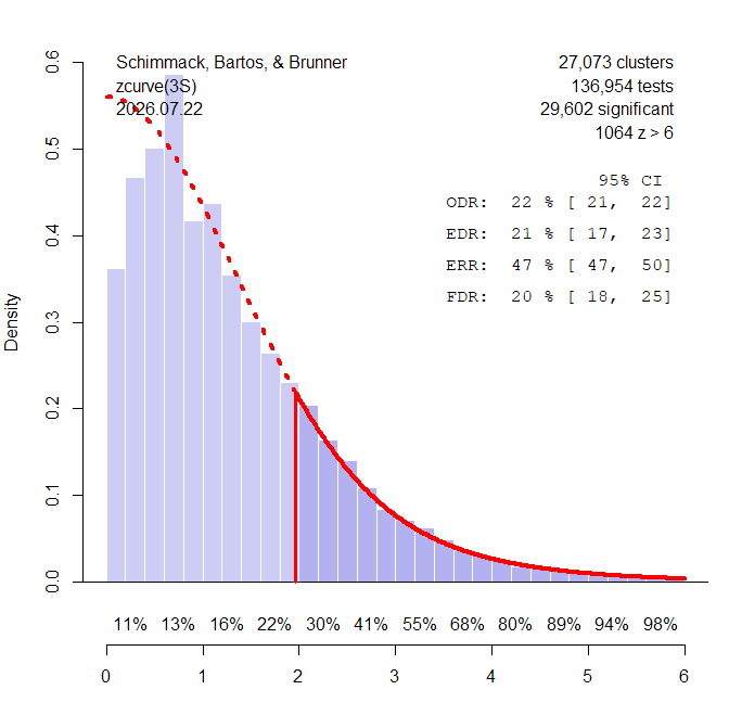
The z-curve plot shows that the mixture closely traces the distribution of significant results. It also predicts the nonsignificant distribution well. The similarity between the observed and expected discovery rates indicates little evidence of selection for significance in the Cochrane data. This finding is informative in its own right. Nonsignificant trials are not missing from these meta-analyses; they are considerably more common than significant trials. This does not rule out other sources of effect-size inflation, but strong publication selection against nonsignificant trials does not appear to characterize this dataset.

The estimated false discovery risk is approximately 20%, with the upper end of the 95% confidence interval at about 25%. Thus, even when z-curve is fitted with a latent distribution closely resembling the one preferred by van Zwet and colleagues, no more than approximately one quarter of significant findings could be exact-null false discoveries. This result is broadly consistent with our earlier analysis of $p$-values reported in medical-journal abstracts, despite the very different dataset and mixture specification.

Normal mixture with free means

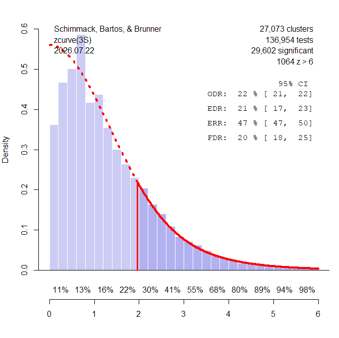
The second model relaxed the assumption that all component means are fixed at zero. Fixing the means at zero served other purposes in van Zwet and colleagues’ application, including producing a symmetric reference distribution and symmetric shrinkage toward zero. However, the restriction could matter if the latent effect distribution were centered or concentrated away from zero.

In the Cochrane data, relaxing the restriction made little difference. The means of the two dominant components were estimated to be close to zero, and the principal z-curve estimates were virtually unchanged. Thus, the zero-mean restriction happens to be fairly benign for these data.

Default discrete z-curve

The third model fitted the default z-curve specification with seven discrete components. Once again, the principal results changed only slightly.

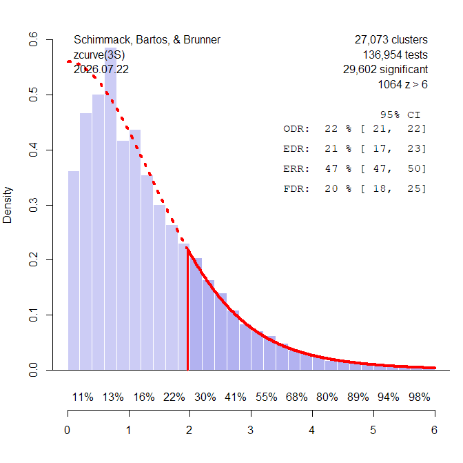
This illustrates an important property of z-curve. Its principal estimands are functions of the fitted distribution of test statistics rather than interpretations of individual mixture components. Different mixture models can assign very different weights and parameters to their latent components while producing nearly identical fitted densities. If they reproduce the relevant distribution of $z$-values equally well, they can therefore produce very similar estimates of the expected discovery rate, expected replication rate, and false discovery risk.

This result directly addresses one aspect of van Zwet’s criticism. A fixed discrete approximation can be biased in some data-generating scenarios, and this possibility should not be ignored. But zcurve3 makes the concern empirically testable. Researchers can fit alternative mixture specifications as a sensitivity analysis. In the Cochrane data, replacing the traditional discrete mixture with normal mixtures does not materially alter the principal z-curve conclusions.

Robust estimands, unstable components

The picture changes when the individual mixture components themselves are interpreted as latent populations.

In the two continuous normal-mixture models, the probability of an effect being exactly zero is zero by construction. The actual exact-null FDR is therefore zero under these models. This should not be confused with the false discovery risk, which remains around 20%. The latter asks how high the FDR could be without assuming that the chosen continuous latent model is literally true.

The zero-centered and free-mean normal mixtures imply false-sign rates of approximately 3.2%, reasonably close to van Zwet et al.’s reported estimate of about 2%.

The default discrete z-curve gives a different latent interpretation. About 4.5% of significant results are assigned to the component with a noncentrality parameter of zero. If this component is interpreted literally, the estimated actual FDR is therefore about 4.5%. If, instead, the zero component is regarded as a discrete approximation to a continuous collection of very small positive and negative effects, exact-zero FDR disappears and approximately half of the significant results in this component become sign errors. Under this interpretation, the false-sign rate is approximately 2.7%.

Thus, these relatively flexible models all imply a false-sign rate below about 5%. However, this apparent agreement should not be mistaken for identification of the latent distribution.

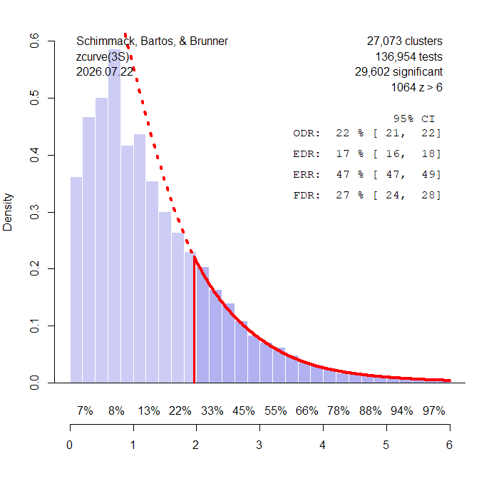
To illustrate the problem, I fitted another discrete mixture with components at noncentralities $0,2,4,$ and $6$. Removing the component at $z=1$ prevents the model from representing weak positive effects explicitly. Many of the low-power studies must therefore be assigned to the zero component instead.

The principal z-curve estimands changed only slightly. The latent interpretation changed dramatically. After accounting for significant observations above $z=6$, the zero component implies an actual FDR of approximately 23%, close to the maximum FDR permitted by the discovery rate. If the zero component is instead interpreted as a symmetric collection of effects extremely close to zero, approximately half of these findings have the wrong sign, producing an estimated false-sign rate of about 11.5%.

Nothing about the observed Cochrane data changed. Only the latent mixture specification changed.

This example illustrates why fitted mixture components should not automatically be interpreted as literal data-generating populations. Their main statistical advantage is precisely their flexibility: different mixtures can approximate the same observed density. Quantities that depend mainly on the fitted density can therefore be robust even when the decomposition into latent components is not. In contrast, quantities that require a literal interpretation of the components—including estimates of the actual proportion of exact zeros, false-sign rates, and some shrinkage quantities—can be substantially more model dependent.

This is not unique to z-curve. Stephens’s (2017) empirical-Bayes approach to false-sign rates, for example, obtains greater stability by imposing a substantive shape constraint: the latent effect distribution is assumed to be unimodal with its mode at zero. Such assumptions may be reasonable, but estimates obtained from them are conditional on those assumptions rather than determined by the observed data alone.

Conclusion

Mixture models remain relatively uncommon in meta-analysis and meta-science, and their use can invite a basic misunderstanding. The most serious mistake is to interpret the fitted components as if they were empirically identified populations of studies or true effects. Component locations, variances, and weights can be highly sensitive to model specification. Different mixtures can fit essentially the same observed distribution while implying substantially different latent decompositions. Good model fit alone therefore cannot establish that one particular decomposition is the true data-generating process.

Z-curve was designed to avoid relying on this interpretation. Its principal estimands—the expected discovery rate and expected replication rate—are global properties of the fitted distribution. The false discovery risk is subsequently obtained from the estimated discovery rate using Sorić’s bound. Consequently, substantially different mixture specifications can produce similar answers as long as they reproduce the relevant features of the observed distribution.

This distinction also clarifies the role of the nil hypothesis. It is not necessary to assume that some fixed proportion of scientific effects are literally zero in order to use false-discovery risk as a credibility criterion. If exact-zero effects do not exist, the actual exact-null FDR is zero. The Sorić bound remains useful because it asks the more conservative question: given the discovery rate, how large could the false discovery rate be? This is consistent with the broader logic of false-discovery methods already established in large-scale multiple testing.

The same point helps clarify discussions of “low power.” Van Zwet and colleagues define the signal-to-noise ratio as the true effect divided by its standard error and translate it into conventional power to reject $H_0:\theta=0$. This is mathematically legitimate, but if exact-zero effects are assumed never to occur, low power against zero cannot itself imply that significant findings are false. It primarily signals that effects are small relative to their sampling error, which creates imprecise estimates, magnitude exaggeration after selection, and some risk of sign errors. How much of this makes a study scientifically untrustworthy requires an explicit criterion.

The present Cochrane analysis provides one such criterion. Across substantially different mixture specifications, the estimated discovery and replication rates and the maximum false discovery rate are remarkably stable. In contrast, actual FDR and false-sign estimates can change substantially when the latent components are interpreted literally.

The lesson is therefore not that one mixture model is correct and another is wrong. Conclusions should be trusted to the extent that they survive reasonable changes in mixture specification. In the Cochrane data, the principal z-curve estimands pass this test. Literal interpretations of the latent mixture components do not.

References

Bartoš F, Schimmack U. Z-curve 2.0: Estimating replication rates and discovery rates. Meta-Psychology. 2022;6:2021.2720. doi:10.15626/MP.2021.2720.

Benjamini Y, Hochberg Y. Controlling the false discovery rate: A practical and powerful approach to multiple testing. J R Stat Soc Series B. 1995;57:289–300. doi:10.1111/j.2517-6161.1995.tb02031.x.

Gelman A, Carlin JB. Beyond power calculations: Assessing Type S (sign) and Type M (magnitude) errors. Perspect Psychol Sci. 2014;9:641–651. doi:10.1177/1745691614551642.

Gelman A, O’Rourke K. Discussion: Difficulties in making inferences about scientific truth from distributions of published p-values. Biostatistics. 2014;15:18–23. doi:10.1093/biostatistics/kxt034.

Ioannidis JPA. Why most published research findings are false. PLoS Med. 2005;2:e124. doi:10.1371/journal.pmed.0020124.

Ioannidis JPA. Discussion: Why “An estimate of the science-wise false discovery rate and application to the top medical literature” is false. Biostatistics. 2014;15:28–36. doi:10.1093/biostatistics/kxt036.

Jager LR, Leek JT. An estimate of the science-wise false discovery rate and application to the top medical literature. Biostatistics. 2014;15:1–12. doi:10.1093/biostatistics/kxt007.

Schimmack U, Bartoš F. Estimating the false discovery risk of (randomized) clinical trials in medical journals based on published p-values. PLoS ONE. 2023;18:e0290084. doi:10.1371/journal.pone.0290084.

Sorić B. Statistical “discoveries” and effect-size estimation. J Am Stat Assoc. 1989;84:608–610. doi:10.2307/2289950.

Stephens M. False discovery rates: A new deal. Biostatistics. 2017;18:275–294. doi:10.1093/biostatistics/kxw041.

Storey JD. The positive false discovery rate: A Bayesian interpretation and the q-value. Ann Stat. 2003;31:2013–2035. doi:10.1214/aos/1074290335.