Scientific progress depends on criticism, especially when it is used to identify limitations of statistical methods and to improve them. z-curve is no exception. Over the past year, several critiques have raised questions about the robustness of z-curve estimates, particularly with respect to the expected discovery rate (EDR). These critiques deserve careful examination, but they also require accurate characterization of what z-curve assumes, what it estimates, and under which conditions its estimates are informative.
Two recent lines of criticism are worth distinguishing. First, Pek et al. (2025) show that z-curve estimates can be biased when the publication process deviates from the assumed selection model. The default z-curve model assumes that selection operates primarily on statistical significance at the conventional α = .05 threshold (z = 1.96). Pek et al. demonstrate that if researchers also suppress statistically significant results with small effect sizes—for example, not publishing a result with p = .04 because the standardized mean difference is only d = .40—then z-curve estimates can become optimistic. This result is correct: z-curve cannot diagnose selective reporting based on effect size rather than statistical significance.
There is limited direct evidence that routine selection on effect-size magnitude (beyond statistical significance) is widespread; the QRPs most commonly reported in self-surveys are largely significance-focused (John et al., 2012). In any case, imperfect correction is not a reason to ignore selection bias entirely, because uncorrected meta-analyses can markedly overestimate population effects and replicability (Carter et al., 2019).
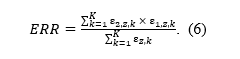
Moreover, the selection mechanism examined by Pek et al. has a clear directional implication: when statistically significant results are additionally filtered by effect size, z-curve’s estimates of EDR and ERR can be biased upward. This matters for interpretation. If z-curve already yields low EDR or ERR estimates, then the type of misspecification studied by Pek et al. would, if present in practice, imply that the underlying parameters could be even lower. For example, an estimated EDR of 20% under the default selection model could correspond to a substantially lower true discovery rate if significant-but-small effects are systematically suppressed. Whether such effect-size–based suppression is common enough to materially affect typical applications remains an empirical question.
A second critique has been advanced by Erik van Zwet, a biostatistician who has applied models of z-value distributions developed in genomics to meta-analyses of medical trials. These models were designed for settings in which the full set of test statistics is observed and therefore do not incorporate selection bias. When applied to literatures where selection bias is present, such models can yield biased estimates. In contrast, z-curve is explicitly designed to assess the presence of selection bias and to correct for it, when it is present. When no bias is present, z-curve can also be fitted to the full z-curve, including non-significant results.
van Zwet has published a few blog posts arguing that z-curve performs poorly when estimating the expected discovery rate (EDR). Importantly, his simulations do not show problems for the expected replication rate (ERR). Thus, z-curve’s ability to estimate the average true power of published significant results is not in question. The disputed issue concerns inference about the broader population of studies, including unpublished nonsignificant results.
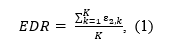
Some aspects of this critique require clarification. van Zwet has suggested that z-curve was evaluated only in a small number of simulations. This is incorrect. Prior work includes two large simulation studies—one conducted by František Bartoš and one conducted by me—that examined EDR confidence-interval coverage across a wide range of conditions. Based on these results, the width of the nominal 95% confidence intervals was conservatively expanded by ±5 percentage points to achieve near-nominal coverage across a wide range of realistic scenarios (see details below). Thus, EDR interval estimation was already empirically validated across many conditions with 100 or more significant results.
However, these simulations did not examine performance of z-curve with small sets of significant results. Because z-curve can technically be fit with as few as 10 significant results, it is reasonable to ask whether EDR confidence-interval coverage remains adequate when the number of significant studies is substantially smaller than 100. To address this question directly, I conducted a new simulation study focusing on the case of 50 significant results.
In addition, I introduced two diagnostics designed to assess when EDR estimation is likely to be weakly identified. Estimation of the EDR relies disproportionately on significant results from low-powered studies or false positives, because these observations provide information about the number of missing nonsignificant results. When nearly all significant results come from highly powered studies, the observed z-value distribution contains little information about what is missing. The first diagnostic therefore counts how many significant z-values fall in the interval from 1.96 to 2.96. Very small counts in this range signal that EDR estimates are driven by limited information. The second diagnostic examines the slope of the z-value density in this interval. A decreasing slope indicates information consistent with a mixture that includes low-powered studies, whereas an increasing slope reflects dominance of high-powered studies and weak identification of the EDR.
Reproducible Results of Simulation Study with 50 Significant Results
The simulation used a fully crossed factorial design with four values for each of four parameters, yielding 192 conditions. Population-level standardized mean differences were set to 0, .2, .4, or .6. Heterogeneity was modeled using normally distributed effect sizes with standard deviations (τ) of 0, .2, .4, or .6. In addition, a separate population of true null studies was included, with the proportion of false discoveries among significant results set to 0, .2, .4, or .6. Sample sizes varied across conditions, starting at n = 50 (25 observations per group). For each condition, simulations were run with exactly 50 significant results.
The simulation code is available here. The results are available here.
Across all scenarios coverage is 96%. The percentage is higher than the nominal 95% because the conservative adjustment leads to higher coverage in less changing scenarios.
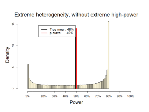
The slope diagnostic works as expected. When the slope is decreasing, coverage is 97%, but when the slope is increasing it drops to 83%. Increasing slopes are more likely to lead to an overestimation than underestimation of the EDR (75%). Increasing slopes occurred in only 5% of all simulations because these scenarios assume that the majority of studies have over 50% power, which requires large samples and moderate to large effect sizes.
The number of z-values in the range between 1.96 and 2.96 also matters. At least 12 values in this range are needed to have 95% coverage. However, the slope criterion is more diagnostic than the number of z-values in this range.
A logistic regression with CI coverage (yes = 1, no = 0) as outcome and slope direction, d, SD, se 2/sqrt(N), and FDR proportion as predictors showed a strong effect of slope direction, FDR, and a slope direction x FDR interaction. Based on these results, I limited the analysis to scenarios with decreasing or flat slopes.
The effect of FDR remained significant (b = 3.55, SE = 1.47), as did the main effect of effect size (b = −2.33, SE = 1.01) and the effect size × SD interaction (b = 6.93, SE = 2.99), indicating systematic variation in coverage across conditions.
These effects are explained by how the design parameters shape the distribution of observed z-values in the critical range used to estimate the EDR (1.96–2.96). Higher FDR values imply a larger proportion of true null effects, which produces a steeper declining slope in the truncated z-distribution and increases information about the mass of missing non-significant results. In contrast, larger effect sizes generate a greater share of high-powered studies with z-values well above the truncation point, which reduces the relative influence of marginally significant results and makes the EDR less identifiable from the observed distribution.
The significant effect size × SD interaction reflects the moderating role of heterogeneity. When heterogeneity is present, even large average effect sizes produce a mixture of moderate- and high-power studies, increasing the density of z-values near the significance threshold and partially restoring information about missing results. As a consequence, the adverse effect of large average effect sizes on coverage is attenuated when heterogeneity is non-zero.
Overall, the most challenging scenarios for EDR estimation are characterized by low heterogeneity and shallow slopes in the just-significant range. In these settings, the observed z-distribution contains limited information about the unobserved, non-significant portion of the distribution, so EDR is weakly identified from the selected data alone.
Inspection of the 192 design cells indicates that the largest coverage shortfalls are concentrated in homogeneous conditions, especially when SD = 0 and FDR = 0. This limitation of the default discrete mixture approximation under near-homogeneity has been documented previously (Brunner & Schimmack, 2020). In practice, it can be addressed by fitting a homogeneity-appropriate specification, such as a single-component model with a free mean and normally distributed heterogeneity (with SD allowed to approach 0), as implemented in z-curve 3.0.
Restricting attention to scenarios with heterogeneous data (SD > .2), 89% of conditions achieved at least 95% coverage, and only 2 conditions (1.4%) fell below 90% coverage. Thus, even with adjusted confidence intervals, nominal coverage is not guaranteed in all edge cases. The remaining coverage problems arise for two reasons: (a) the selected z-distribution can be nearly uninformative about the amount of missing, non-significant evidence when the just-significant slope is shallow, and (b) the default heterogeneous specification can be misspecified when applied to approximately homogeneous data. A conservative approach to the lower coverage in some cases is to report the results as 85% confidence interval even if coverage on average is over 95%.
Conclusion
Pek et al. and van Zwet have raised broad concerns about z-curve’s estimates of the expected discovery rate (EDR), which is used to assess publication bias and to quantify the extent of missing nonsignificant results. Their arguments rely heavily on a small set of stylized scenarios. These scenarios do not show that z-curve generally produces untrustworthy results. In contrast, prior large-scale simulation studies, together with the present extension to datasets with only 50 significant results, indicate that z-curve’s EDR confidence intervals achieve near-nominal coverage across a wide range of conditions, including many that are plausible for applied research.
Importantly, the new simulations also validate simple diagnostics that indicate when EDR estimation is likely to be less reliable. In particular, the shape of the significant z-value distribution in the critical range from 1.96 to 2.96—especially whether the density decreases or increases just above the significance threshold—helps identify weak-information regimes in which EDR may be overestimated and confidence-interval coverage may be reduced. Users can therefore compare the near-threshold shape of their observed z-value distribution to the patterns observed in simulation to assess whether EDR should be interpreted cautiously in a given application.
Overall, these results support the conclusion that z-curve provides credible estimates of the expected replication rate (ERR) and, under diagnostically identifiable conditions, the expected discovery rate (EDR), and that these quantities remain useful for evaluating the credibility of literatures in which selection on statistical significance is present.
The pattern is now familiar. I received another anonymous review by Reviewer 2 from a z-curve article that repeated Pek’s concerns about the performance of z-curve. To deal with biased reviewers, journals allow authors to mention potentially biased reviewers. I suggest doing so for Pek. I also suggest sharing a manuscript with me to ensure proper interpretation of results and to make it “reviewer-safe.”
To justify the claim that Pek is biased, researchers can use this rebuttal of Pek’s unscientific claims about z-curve.
Reviewer 2 (either Pek or a Pek parrot)
Reviewer Report:
The manuscript “A review and z-curve analysis of research on the palliative association of system justification” (Manuscript ID 1598066) extends the work of Sotola and Credé (2022), who used Z-curve analysis to evaluate the evidential value of findings related to system justification theory (SJT). The present paper similarly reports estimates of publication bias, questionable research practices (QRPs), and replication rates in the SJT literature using Z-curve. Evaluating how scientific evidence accumulates in the published literature is unquestionably important.
However, there is growing concern about the performance of meta-analytic forensic tools such as p-curve (Simonsohn, Nelson, & Simmons, 2014; see Morey & Davis-Stober, 2025 for a critique) and Z-curve (Brunner & Schimmack, 2020; Bartoš & Schimmack, 2022; see Pek et al., in press for a critique). Independent simulation studies increasingly suggest that these methods may perform poorly under realistic conditions, potentially yielding misleading results.
Justification for a theory or method typically requires subjecting it to a severe test (Mayo, 2019) – that is, assuming the opposite of what one seeks to establish (e.g., a null hypothesis of no effect) and demonstrating that this assumption leads to contradiction. In contrast, the simulation work used to support Z-curve (Brunner & Schimmack, 2020; Bartoš & Schimmack, 2022) relies on affirming belief through confirmation, a well-documented cognitive bias.
Findings from Pek et al. (in press) show that when selection bias is presented in published p-values — the very scenario Z-curve was intended to be applied — estimates of the expected discovery rate (EDR), expected replication rate (ERR), and Sorić’s False Discovery Risk (FDR) are themselves biased.
The magnitude and direction of this bias depend on multiple factors (e.g., number of p-values, selection mechanism of p-values) and cannot be corrected or detected from empirical data alone. The manuscript’s main contribution rests on the assumption that Z-curve yields reasonable estimates of the “reliability of published studies,” operationalized as a high ERR, and that the difference between the observed discovery rate (ODR) and EDR quantifies the extent of QRPs and publication bias.
The paper reports an ERR of .76, 95% CI [.53, .91] and concludes that research on the palliative hypothesis may be more reliable than findings in many other areas of psychology. There are several issues with this claim. First, the assertion that Sotola (2023) validated ERR estimates from the Z-curve reflects confirmation bias – I have not read Röseler (2023) and cannot comment on the argument made in it. The argument rests solely on the descriptive similarly between the ERR produced by Z-curve and the replication rate reported by the Open Science Collaboration (2015). However, no formal test of equivalence was conducted, and no consideration was given to estimate imprecision, potential bias in the estimates, or the conditions under which such agreement might occur by chance.
At minimum, if Z-curve estimates are treated as predicted values, some form of cross-validation or prediction interval should be used to quantify prediction uncertainty. More broadly, because ERR estimates produced by Z-curve are themselves likely biased (as shown in Pek et al., in press), and because the magnitude and direction of this bias are unknown, comparisons about ERR values across literatures do not provide a strong evidential basis for claims about the relative reliability of research areas.
Furthermore, the width of the 95% CI spans roughly half of the bounded parameter space of [0, 1], indicating substantial imprecision. Any claims based on these estimates should thus be contextualized with appropriate caution.
Another key result concerns the comparison of EDR = .52, 95% CO [.14, .92], and ODR = .81, 95% CI = [.69, .90]. The manuscript states that “When these two estimates are highly discrepant, this is consistent with the presence of questionable research practices (QRPS) and publication bias in this area of research (Brunner & Schimmack, 2020).
But in this case, the 95% CIs for the EDR and ODR in this work overlapped quite a bit, meaning that they may not be significantly different…” (p. 22). There are several issues with such a claim. First, Z curve results cannot directly support claims about the presence of QRPs.
The EDR reflects the proportion of significant p values expected under no selection bias, but it does not identify the source of selection bias (e.g., QRPs, fraud, editorial decisions). Using Z curve requires accepting its assumed missing data mechanism—a strong assumption that cannot be empirically validated.
Second, a descriptive comparison between two estimates cannot be interpreted as a formal test of difference (e.g., eyeballing two estimates of means as different does not tell us whether this difference is not driven by sampling variability). Means can be significantly different even if their confidence intervals overlap (Cumming & Finch, 2005).
A formal test of the difference is required. Third, EDR estimates can be biased. Even under ideal conditions, convergence to the population values requires extremely large numbers of studies (e.g., > 3000, see Figure 1 of Pek et al., in press).
The current study only has 64 tests. Thus, even if a formal test of the difference of ODR – EDR was conducted, little confidence could be placed on the result if the EDR estimate is biased and does not reflect the true population value.
Although I am critical of the outputs of Z curve analysis due to its poor statistical performance under realistic conditions, the manuscript has several strengths. These include adherence to good meta analytic practices such as providing a PRISMA flow chart, clearly stating inclusion and exclusion criteria, and verifying the calculation of p values. These aspects could be further strengthened by reporting test–retest reliability (given that a single author coded all studies) and by explicitly defining the population of selected p values. Because there appears to be heterogeneity in the results, a random effects meta analysis may be appropriate, and study level variables (e.g., type of hypothesis or analysis) could be used to explain between study variability. Additionally, the independence of p values has not been clearly addressed; p values may be correlated within articles or across studies. Minor points: The “reliability” of studies should be explicitly defined. The work by Manapat et al. (2022) should be cited in relation to Nagy et al. (2025). The findings of Simmons et al. (2011) applies only to single studies.
However, most research is published in multi-study sets, and follow-up simulations by Wegener at al. (2024) indicate that the Type I error rate is well-controlled when methodological constraints (e.g., same test, same design, same measures) are applied consistently across multiple studies – thus, the concerns of Simmons et al. (2011) pertain to a very small number of published results.
I could not find the reference to Schimmack and Brunner (2023) cited on p. 17.
Rebuttal to Core Claims in Recent Critiques of z-Curve
1. Claim: z-curve “performs poorly under realistic conditions”
Rebuttal
The claim that z-curve “performs poorly under realistic conditions” is not supported by the full body of available evidence. While recent critiques demonstrate that z-curve estimates—particularly EDR—can be biased under specific data-generating and selection mechanisms, these findings do not justify a general conclusion of poor performance.
Z-curve has been evaluated in extensive simulation studies that examined a wide range of empirically plausible scenarios, including heterogeneous power distributions, mixtures of low- and high-powered studies, varying false-positive rates, different degrees of selection for significance, and multiple shapes of observed z-value distributions (e.g., unimodal, right-skewed, and multimodal distributions). These simulations explicitly included sample sizes as low as k ≈ 100, which is typical for applied meta-research in psychology.
Across these conditions, z-curve demonstrated reasonable statistical properties conditional on its assumptions, including interpretable ERR and EDR estimates and confidence intervals with acceptable coverage in most realistic regimes. Importantly, these studies also identified conditions under which estimation becomes less informative—such as when the observed z-value distribution provides little information about missing nonsignificant results—thereby documenting diagnosable scope limits rather than undifferentiated poor performance.
Recent critiques rely primarily on selective adversarial scenarios and extrapolate from these to broad claims about “realistic conditions,” while not engaging with the earlier simulation literature that systematically evaluated z-curve across a much broader parameter space. A balanced scientific assessment therefore supports a more limited conclusion: z-curve has identifiable limitations and scope conditions, but existing simulation evidence does not support the claim that it generally performs poorly under realistic conditions.
2. Claim: Bias in EDR or ERR renders these estimates uninterpretable or misleading
Rebuttal
The critique conflates the possibility of bias with a lack of inferential value. All methods used to evaluate published literatures under selection—including effect-size meta-analysis, selection models, and Bayesian hierarchical approaches—are biased under some violations of their assumptions. The existence of bias therefore does not imply that an estimator is uninformative.
Z-curve explicitly reports uncertainty through bootstrap confidence intervals, which quantify sampling variability and model uncertainty given the observed data. No evidence is presented that z-curve confidence intervals systematically fail to achieve nominal coverage under conditions relevant to applied analyses. The appropriate conclusion is that z-curve estimates must be interpreted conditionally and cautiously, not that they lack statistical meaning.
This claim overgeneralizes results from specific, highly constrained simulation scenarios. The cited sample sizes correspond to conditions in which the observed data provide little identifying information, not to a general requirement for statistical validity.
In applied statistics, consistency in the limit does not imply that estimates at smaller sample sizes are meaningless; it implies that uncertainty must be acknowledged. In the present application, this uncertainty is explicitly reflected in wide confidence intervals. Small sample sizes therefore affect precision, not validity, and do not justify dismissing the estimates outright.
4. Claim: Differences between ODR and EDR cannot support inferences about selection or questionable research practices
Rebuttal
It is correct that differences between ODR and EDR do not identify the source of selection (e.g., QRPs, editorial decisions, or other mechanisms). However, the critique goes further by implying that such differences lack diagnostic value altogether.
Under the z-curve framework, ODR–EDR discrepancies are interpreted as evidence of selection, not of specific researcher behaviors. This inference is explicitly conditional and does not rely on attributing intent or mechanism. Rejecting this interpretation would require demonstrating that ODR–EDR differences are uninformative even under monotonic selection on statistical significance, which has not been shown.
5. Claim: ERR comparisons across literatures lack evidential basis because bias direction is unknown
Rebuttal
The critique asserts that because ERR estimates may be biased with unknown direction, comparisons across literatures lack evidential value. This conclusion does not follow.
Bias does not eliminate comparative information unless it is shown to be large, variable, and systematically distorting rankings across plausible conditions. No evidence is provided that ERR estimates reverse ordering across literatures or are less informative than alternative metrics. While comparative claims should be interpreted cautiously, caution does not imply the absence of evidential content.
6. Claim: z-curve validation relies on “affirming belief through confirmation”
Rebuttal
This characterization misrepresents the role of simulation studies in statistical methodology. Simulation-based evaluation of estimators under known data-generating processes is the standard approach for assessing bias, variance, and coverage across frequentist and Bayesian methods alike.
Characterizing simulation-based validation as epistemically deficient would apply equally to conventional meta-analysis, selection models, and hierarchical Bayesian approaches. No alternative validation framework is proposed that would avoid reliance on model-based simulation.
7. Implicit claim: Effect-size meta-analysis provides a firmer basis for credibility assessment
Rebuttal
Effect-size meta-analysis addresses a different inferential target. It presupposes that studies estimate commensurable effects of a common hypothesis. In heterogeneous literatures, pooled effect sizes represent averages over substantively distinct estimands and may lack clear interpretation.
Moreover, effect-size meta-analysis does not estimate discovery rates, replication probabilities, or false-positive risk, nor does it model selection unless explicitly extended. No evidence is provided that effect-size meta-analysis offers superior performance for evaluating evidential credibility under selective reporting.
Summary
The critiques correctly identify that z-curve is a model-based method with assumptions and scope conditions. However, they systematically extend these points beyond what the evidence supports by:
extrapolating from selective adversarial simulations,
conflating potential bias with lack of inferential value,
overgeneralizing small-sample limitations,
and applying asymmetrical standards relative to conventional methods.
A scientifically justified conclusion is that z-curve provides conditionally informative estimates with quantifiable uncertainty, not that it lacks statistical validity or evidential relevance.
Bartoš, F., & Schimmack, U. (2022). Z-curve 2.0: Estimating replication rates and discovery rates. Meta-Psychology, 6, Article e0000130. https://doi.org/10.15626/MP.2022.2981
Brunner, J., & Schimmack, U. (2020). Estimating population mean power under conditions of heterogeneity and selection for significance. Meta- Psychology. MP.2018.874, https://doi.org/10.15626/MP.2018.874
van Zwet, E., Gelman, A., Greenland, S., Imbens, G., Schwab, S., & Goodman, S. N. (2024). A New Look at P Values for Randomized Clinical Trials. NEJM evidence, 3(1), EVIDoa2300003. https://doi.org/10.1056/EVIDoa2300003
The Story of Two Z-Curve Models
Erik van Zwet recently posted a critique of the z-curve method on Andrew Gelman’s blog.
Meaningful discussion of the severity and scope of this critique was difficult in that forum, so I address the issue more carefully here.
van Zwet identified a situation in which z-curve can overestimate the Expected Discovery Rate (EDR) when it is inferred from the distribution of statistically significant z-values. Specifically, when the distribution of significant results is driven primarily by studies with high power, the observed distribution contains little information about the distribution of nonsignificant results. If those nonsignificant results are not reported and z-curve is nevertheless used to infer them from the significant results alone, the method can underestimate the number of missing nonsignificant studies and, as a consequence, overestimate the Expected Discovery Rate (EDR).
This is a genuine limitation, but it is a conditional and diagnosable one. Crucially, the problematic scenarios are directly observable in the data. Problematic data have an increasing or flat slope of the significant z-value distribution and a mode well above the significance threshold. In such cases, z-curve does not silently fail; it signals that inference about missing studies is weak and that EDR estimates should not be trusted.
This is rarely a problem in psychology, where most studies have low power, the mode is at the significance criterion, and the slope decreases, often steeply. This pattern implies a large set of non-significant results and z-curve provides good estimates in these scenarios. It is difficult to estimate distributions of unobserved data, leading to wide confidence intervals around these estimates. However, there is no fixed number of studies that are needed. The relevant question is whether the confidence intervals are informative enough to support meaningful conclusions.
One of the most powerful set of studies that I have actually seen comes from epidemiology, where studies often have large samples to estimate effect sizes precisely. In these studies, power to reject the null hypothesis is actually not really important, but the data serve as a good example of a set of studies with high power, rather than low power as in psychology.
However, even this example shows a decreasing slope and a mode at significance criterion. Fitting z-curve to these data still suggests some selection bias and no underestimation of reported non-significant results. This illustrates how extreme van Zwet’s scenario must be to produce the increasing-slope pattern that undermines EDR estimation.
What about van Zwet’s Z-Curve Method?
It is also noteworthy that van Zwet does not compare our z-curve method (Bartos & Schimmack, 2022; Brunner & Bartos, 2020) to his own z-curve method that was used to analyze z-values from clinical trials (van Zwet et al., 2024).
The article fits a model to the distribution of absolute z-values (ignoring whether results show a benefit or harm to patients). The key differences between the two approaches are that (a) van Zwet et al.’s model uses all z-values and assumes (implicitly) that there is no selection bias, and (b) that true effect sizes are never zero and errors can only be sign errors. Based on these assumptions, the article concludes that no more than 2% of clinical trials produce a result that falsely rejects a true hypothesis. For example, a statistically significant result could be treated as an error only if the true effect has the opposite sign (e.g., the true effect increases smoking, but a significant result is used to claim it reduced smoking).
The advantage of this method is that it is not necessary to estimate the EDR from the distribution of only significant results, but it does so only by assuming that publication bias does not exist. In this case, we can just count the observed non-significant and significant results and use the observed discovery rate to estimate average power and the false positive risk.
The trade-off is clear. z-curve attempts to address selection bias and sometimes lacks sufficient information to do so reliably; van Zwet’s approach achieves stable estimates by assuming the problem away. The former risks imprecision when information is weak; the latter risks bias when its core assumption is violated.
In the example from epidemiology, there is evidence of some publication bias and omission of non-significant results. Using van Zwet’s model would be inappropriate because it would overestimate the true discovery rate. The focus on sign errors alone is also questionable and should be clearly stated as a strong assumption. It implies that significant results in the right direction are not errors, even if effect sizes are close to zero. For example, a significant result that suggests it extends life is considered a true finding, even if the effect size is one day.
False positive rates do not fully solve that problem, but false positive rates that include zero as a hypothetical value for the population effect size are higher and treat small effects close to zero as errors rather than treating half of them as correct rejections of the null hypothesis. For example, an intervention that decreases smoking by 1% of all smokers is not really different from one that increases it by 1%, but a focus on signs treats only the latter one as an error.
In short, van Zwet’s critique identifies a boundary condition for z-curve, not a general failure. At the same time, his own method rests on a stronger and untested assumption—no selection bias—whose violation would invalidate its conclusions entirely. No method is perfect and using a single scenario to imply that a method is always wrong is not a valid argument against any method. By the same logic, van Zwet’s own method could be declared “useless” whenever selection bias exists, which is precisely the point: all methods have scope conditions.
Using proper logic, we suggest that all methods work when assumptions are met. The main point is to test whether they are met or not. We clarified that z-curve estimation of the EDR assumes that enough low powered studies produced significant results to influence the distribution of significant results. If the slope of significant results is not decreasing, this assumption does not hold and z-curve should not be used to estimate the EDR. Similarly, users of van Zwets first method should first test whether selection bias is present and not use it when it does. They should also examine whether they think a proportion of studies could have tested practically true null hypotheses and not use the method when this is a concern.
Finally, the blog post responds to Gelman’s polemic about our z-curve method and earlier work by Jager and Leek (2014), by noting that Gelman’s critic of other methods exist in parallel to his own work (at least co-authorship) that also modeled distribution of z-values to make claims about power and the risk of false inferences. The assumption of this model that selection bias does not exist is peculiar, given Gelman’s typical writing about low power and the negative effects of selection for significance. A more constructive discussion would apply the same critical standards to all methods—including one’s own.
Wilson BM, Wixted JT. The Prior Odds of Testing a True Effect in Cognitive and Social Psychology. Advances in Methods and Practices in Psychological Science. 2018;1(2):186-197. doi:10.1177/2515245918767122
Abstract
Wilson and Wixted had a cool idea, but it turns out to be wrong. They proposed that sign errors in replication studies can be used to estimate false positive rates. Here I show that their approach makes a false assumption and does not work.
Introduction
Two influential articles shifted concerns about false positives in psychology from complacency to fear (Ioannidis, 2005; Simmons, Nelson, & Simonsohn, 2011). First, psychologists assumed that false rejections of the null hypothesis (no effect) are rare because the null hypothesis is rarely true. Effects were either positive or negative, but never really zero. In addition, meta-analyses typically found evidence for effects, even assuming biased reporting of studies (Rosenthal, 1979).
Simmons et al. (2011) demonstrated, however, that questionable, but widely used statistical practices can increase the risk of publishing significant results without real effects from the nominal 5% level (p < .05) to levels that may exceed 50% in some scenarios. When only 25% of significant results in social psychology could be replicated, it seemed possible that a large number of the replication failures were false positives (Open Science Collaboration, 2015).
Wilson and Wixted (2018) used the reproducibility results to estimate how often social psychologists test true null hypotheses. Their approach relied on the rate of sign reversals between original and replication estimates. If the null hypothesis is true, sampling error will produce an equal number of estimates in both directions. Thus, a high rate of sign reversals could be interpreted as evidence that many original findings reflect sampling error around a true null. Second, for every sign reversal there is typically a same-sign replication, and Wilson and Wixted treated the remaining same-sign results as reflecting tests of true hypotheses that reliably produce the correct sign.
Let P(SR) be the observed proportion of sign reversals between originals and replications (not conditional on significance). If true effects always reproduce the same sign and null effects produce sign reversals 50% of the time, then the observed SR provides an estimate of the proportion of true null hypotheses that were tested, P(True-H0).
P(True-H0) = 2*P(SR)
Wilson and Wixted further interpreted this quantity as informative about the fraction of statistically significant original results that might be false positives. Wilson and Wixted (2018) found approximately 25% sign reversals in replications of social psychological studies. Under their simplifying assumptions, this implies 50% true null hypotheses in the underlying set of hypotheses being tested, and they used this inference, together with assumptions about significance and power, to argue that false positives could be common in social psychology.
Like others, I thought this was a clever way to make use of sign reversals. The article has been cited only 31 times (WoS, January 6, 2026), and none of the articles critically examined Wilson and Wixted’s use of sign errors to estimate false positive rates.
However, other evidence suggested that false positives are rare (Schimmack, 2026). To resolve the conflict between Wilson and Wixted’s conclusions and other findings, I reexamined their logic and ChatGPT pointed out Wilson and Wixted’s (2018) formula rests on assumptions that need not hold.
The main reason is that it makes the false assumption that tests of true hypotheses do not produce sign errors. This is simply false because studies that test false null hypotheses with low power can still produce sign reversals (Gelman & Carlin, 2014). Moreover, sign reversals can be generated even when the false-positive rate is essentially zero, if original studies are selected for statistical significance and the underlying studies have low power. In fact, it is possible to predict the percentage of sign reversals from the non-centrality of the test statistic under the assumption that all studies have the same power. To obtain 25% sign reversals, all studies could test a false null hypothesis with about 10% power. In that scenario, many replications would reverse sign because estimates are highly noisy, while the original literature could still contain few or no literal false positives if the true effects are nonzero.
Empirical Examination with Many Labs 5
I used the results from ManyLabs5 (Ebersole et al., 2020) to evaluate what different methods imply about the false discovery risk of social psychological studies in the Reproducibility Project, first applying Wilson and Wixted’s sign-reversal approach and then using z-curve (Bartos & Schimmack, 2022; Brunner & Schimmack, 2020).
ManyLabs5 conducted additional replications of 10 social psychological studies that failed to replicate in the Reproducibility Project (Open Science Collaboration, 2015). The replication effort included both the original Reproducibility Project protocols and revised protocols developed in collaboration with the original authors. There were 7 sign reversals in total across the 30 replication estimates. Using Wilson and Wixted’s sign-reversal framework, 7 out of 30 sign reversals (23%) would be interpreted as evidence that approximately 46% of the underlying population effects in this set are modeled as exactly zero (i.e., that H0 is true for about 46% of the effects).
To compare these results more directly to Wilson and Wixted’s analysis, it is necessary to condition on non-significant replication outcomes, because ManyLabs5 selected studies based on replication failure rather than original significance alone. Among the non-significant replication results, 25 sign reversals occurred out of 75 estimates, corresponding to a rate of 33%, which would imply a false-positive rate of approximately 66% under Wilson and Wixted’s framework. Although this estimate is somewhat higher, both analyses would be interpreted as implying a large fraction of false positives—on the order of one-half—among the original significant findings within that framework.
To conduct a z-curve analysis, I transformed the effect sizes (r) in ManyLabs5 (Table 3) into d-values and used the reported confidence intervals to compute standard errors, SE = (d upper − d lower)/3.92, and corresponding z-values, z = d/SE. I fitted a z-curve model that allows for selection on statistical significance (Bartos & Schimmack, 2022; Brunner & Schimmack, 2020) to the 10 significant original results. I fitted a second z-curve model to the 30 replication results, treating this set as unselected (i.e., without modeling selection on significance).
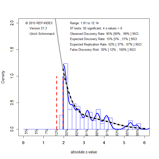
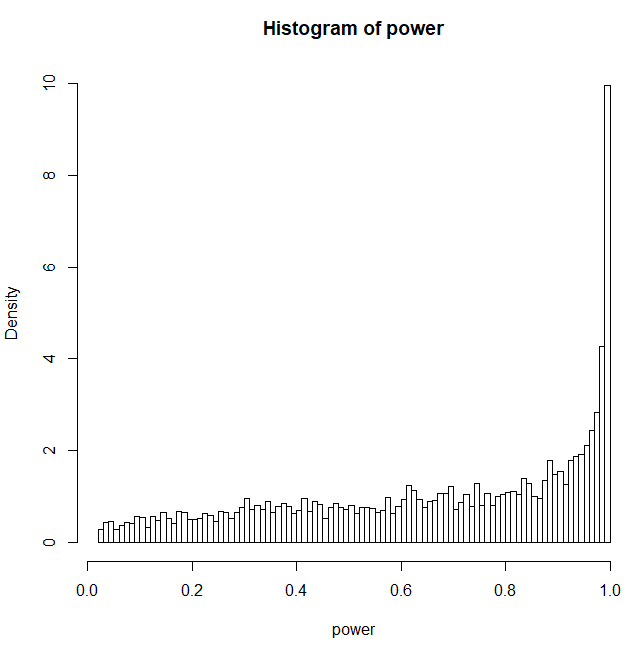
The z-curve for the 10 original results shows evidence consistent with strong selection on statistical significance, despite the small set of studies. Although all original results are statistically significant, the estimated expected discovery rate is only 8%, and the upper limit of the 95% confidence interval is 61%, well below 100%. Visual inspection of the z-curve plot also shows a concentration of results just above the significance threshold (z = 1.96) and none just below it, even though sampling variation does not create a discontinuity between results with p = .04 and p = .06.
The expected replication rate (ERR) is a model-based estimate of the average probability that an exact replication would yield a statistically significant result in the same direction. For the 10 original studies, ERR is 32%, but the confidence interval is wide (3% to 70%). The lower bound near 3% is close to the directional false-alarm rate under a two-sided test when the true effect is zero (α/2 = 2.5%), meaning that the data are compatible with the extreme-null scenario in which all underlying effects are zero and the original significant results reflect selection. This does not constitute an estimate of the false-positive rate; rather, it indicates that the data are too limited to rule out that worst-case possibility. At the same time, the same results are also compatible with an alternative scenario in which all underlying effects are non-zero but power is low across studies.
For the 30 replication results, the z-curve model provides a reasonable fit to the observed distribution, which supports the use of a model that does not assume selection on statistical significance. In this context, the key quantity is the expected discovery rate (EDR), which can be interpreted as a model-based estimate of the average true power of the 30 replication studies. The estimated EDR is 17%. This value is lower than the corresponding estimate based on the original studies, despite increases in sample sizes and statistical power in the replication attempts. This pattern illustrates that ERR estimates derived from biased original studies tend to be overly optimistic predictors of actual replication outcomes (Bartos & Schimmack, 2022). In contrast, the average power of the replication studies can be estimated more directly because the model does not need to correct for selection bias.
A key implication is that the observed rate of sign reversals (23%) could have been generated by a set of studies in which all null hypotheses are false but average power is low (around 17%). However, the z-curve analysis also shows that even a sample of 30 studies is insufficient to draw precise conclusions about false positive rates in social psychology. Following Sorić (1989), the EDR can be used to derive an upper bound on the false discovery rate (FDR), that is, the maximum proportion of false positives consistent with the observed discovery rate. Based on this approach, the FDR ranges from 11% to 100%. To rule out high false positive risks, studies would need higher power, narrower confidence intervals, or more stringent significance thresholds.
Conclusion
This blog post compared Wilson and Wixted’s use of sign reversals to estimate false discovery rates with z-curve estimates of false discovery risk. I showed that Wilson and Wixted’s approach rests on implausible assumptions. Most importantly, it assumes that sign reversals occur only when the true effect is exactly zero. It does not allow for sign reversals under nonzero effects, which can occur when all null hypotheses are false but tests of these hypotheses have low power.
The z-curve analysis of 30 replication estimates in the ML5 project shows that low average power is a plausible explanation for sign reversals even without invoking a high false-positive rate. Even with the larger samples used in ML5, the data are not precise enough to draw firm conclusions about false positives in social psychology. A key problem remains the fundamental asymmetry of NHST: it makes it possible to reject null hypotheses, but it does not allow researchers to demonstrate that an effect is (practically) zero without very high precision.
The solution is to define the null hypothesis as a region of effect sizes that are so small that they are practically meaningless. The actual level may vary across domains, but a reasonable default is Cohen’s criterion for a small effect size, r = .1 or d = .2. By this criterion, only two of the replication studies in ML5 had sample sizes that were large enough to produce results that ruled out effect sizes of at least r = .1 with adequate precision. Other replications still lacked precision to do so. Interestingly, five of the ten original statistically significant results also failed to rule out effect sizes of at least r = .1, because their confidence intervals included r = .10. Thus, these studies at best provided suggestive evidence about the sign of an effect, but no evidence that the effect size is practically meaningful.
The broader lesson is that any serious discussion of false positives in social psychology requires (a) a specification of what counts as an “absence of an effect” in practice, using minimum effect sizes of interest that can be empirically tested, (b) large sample sizes that allow precise estimation of effect sizes, and (c) unbiased reporting of results. A few registered replication reports come close to this ideal, but even these results have failed to resolve controversies because effect sizes close to zero in the predicted direction remain ambiguous without a clearly specified threshold for practical importance. To avoid endless controversies and futile replication studies, it is necessary to specify minimum effect sizes of interest before data are collected.
In practice, this means designing studies so that the confidence interval can exclude effects larger than the minimum effect size of interest, rather than merely achieving p < .05 against a point null of zero. Conceptually, this is closely related to specifying the null hypothesis as a minimum effect size and using a directional test, rather than using a two-sided test against a nil null of exactly zero. Put differently, the problem is not null hypothesis testing per se, but nil hypothesis testing (Cohen, 1994).
I love talking to ChatGPT because it is actually able to process arguments in a rational manner without motivated biases (at least about topics like average power). The document is a transcript of my discussion with ChatGPT about McShane et al.’s article “Average Power: A Cautionary Note” The article has been cited as “evidence” that average power estimates are useless or even fundamentally flawed. As you can see from the discussion that is an overstatement. Like all estimates of unknown population parameters, it is possible that estimates are biased, but the problems are by no means greater than the problems in estimates of other meta-analytic averages. After offering some arguments in favor of using average power estimates, ChatGPT agrees that it can provide useful information to evaluate the presence of publicatoin bias in original studies and to predict the outcome of replication studies and to evaluate discrepancies in success rates between original and replication studies.
Jerry Brunner is a recent emeritus from the Department of Statistics at the University of Toronto Mississauga. Jerry first started in psychology, but was frustrated by the unscientific practices he observed in graduate school. He went on to become a professor in statistics. Thus, he is not only an expert in statistis. He also understands the methodological problems in psychology.
Sometime in the wake of the replication crisis around 2014/15, I went to his office to talk to him about power and bias detection. . Working with Jerry was educational and motivational. Without him z-curve would not exist. We spend years on trying different methods and thinking about the underlying statistical assumptions. Simulations often shattered our intuitions. The Brunner and Schimmack (2020) article summarizes all of this work.
A few years later, the method is being used to examine the credibility of published articles across different research areas. However, not everybody is happy about a tool that can reveal publication bias, the use of questionable research practices, and a high risk of false positive results. An anonymous reviewer dismissed z-curve results based on a long list of criticisms (Post: Dear Anonymous Reviewer). It was funny to see how ChatGPT responds to these criticisms (Comment). However, the quality of ChatGPT responses is difficult to evaluate. Therefore, I am pleased to share Jerry’s response to the reviewer’s comments here. Let’s just say that the reviewer was wise to make their comments anonymously. Posting the review and the response in public also shows why we need open reviews like the ones published in Meta-Psychology by the reviewers of our z-curve article. Hidden and biased reviews are just one more reason why progress in psychology is so slow.
Jerry Brunner’s Response
This is Jerry Brunner, the “Professor of Statistics” mentioned the post. I am also co-author of Brunner and Schimmack (2020). Since the review Uli posted is mostly an attack on our joint paper (Brunner and Schimmack, 2020), I thought I’d respond.
First of all, z-curve is sort of a moving target. The method described by Brunner and Schimmack is strictly a way of estimating population mean power based on a random sample of tests that have been selected for statistical significance. I’ll call it z-curve 1.0. The algorithm has evolved over time, and the current z-curve R package (available at https://cran.r-project.org/web/packages/zcurve/index.html) implements a variety of diagnostics based on a sample of p-values. The reviewer’s comments apply to z-curve 1.0, and so do my responses. This is good from my perspective, because I was in on the development of z-curve 1.0, and I believe I understand it pretty well. When I refer to z-curve in the material that follows, I mean z-curve 1.0. I do believe z-curve 1.0 has some limitations, but they do not overlap with the ones suggested by the reviewer.
Here are some quotes from the review, followed by my answers.
(1) “… z-curve analysis is based on the concept of using an average power estimate of completed studies (i.e., post hoc power analysis). However, statisticians and methodologists have written about the problem of post hoc power analysis …”
This is not accurate. Post-hoc power analysis is indeed fatally flawed; z-curve is something quite different. For later reference, in the “observed” power method, sample effect size is used to estimate population effect size for a single study. Estimated effect size is combined with observed sample size to produce an estimated non-centrality parameter for the non-central distribution of the test statistic, and estimated power is calculated from that, as an area under the curve of the non-central distribution. So, the observed power method produces an estimated power for an individual study. These estimates have been found to be too noisy for practical use.
The confusion of z-curve with observed power comes up frequently in the reviewer’s comments. To be clear, z-curve does not estimate effect sizes, nor does it produce power estimates for individual studies.
(2) “It should be noted that power is not a property of a (completed) study (fixed data). Power is a performance measure of a procedure (statistical test) applied to an infinite number of studies (random data) represented by a sampling distribution. Thus, what one estimates from completed study is not really “power” that has the properties of a frequentist probability even though the same formula is used. Average power does not solve this ontological problem (i.e., misunderstanding what frequentist probability is; see also McShane et al., 2020). Power should always be about a design for future studies, because power is the probability of the performance of a test (rejecting the null hypothesis) over repeated samples for some specified sample size, effect size, and Type I error rate (see also Greenland et al., 2016; O’Keefe, 2007). z-curve, however, makes use of this problematic concept of average power (for completed studies), which brings to question the validity of z-curve analysis results.”
The reviewer appears to believe that once the results of a study are in, the study no longer has a power. To clear up this misconception, I will describe the model on which z-curve is based.
There is a population of studies, each with its own subject population. One designated significance test will be carried out on the data for each study. Given the subject population, the procedure and design of the study (including sample size), significance level and the statistical test employed, there is a probability of rejecting the null hypothesis. This probability has the usual frequentist interpretation; it’s the long-term relative frequency of rejection based on (hypothetical) repeated sampling from the particular subject population. I will use the term “power” for the probability of rejecting the null hypothesis, whether or not the null hypothesis is exactly true.
Note that the power of the test — again, a member of a population of tests — is a function of the design and procedure of the study, and also of the true state of affairs in the subject population (say, as captured by effect size).
So, every study in the population of studies has a power. It’s the same before any data are collected, and after the data are collected. If the study were replicated exactly with a fresh sample from the same population, the probability of observing significant results would be exactly the power of the study — the true power.
This takes care of the reviewer’s objection, but let me continue describing our model, because the details will be useful later.
For each study in the population of studies, a random sample is drawn from the subject population, and the null hypothesis is tested. The results are either significant, or not. If the results are not significant, they are rejected for publication, or more likely never submitted. They go into the mythical “file drawer,” and are no longer available. The studies that do obtain significant results form a sub-population of the original population of studies. Naturally, each of these studies has a true power value. What z-curve is trying to estimate is the population mean power of the studies with significant results.
So, we draw a random sample from the population of studies with significant results, and use the reported results to estimate population mean power — not of the original population of studies, but only of the subset that obtained significant results. To us, this roughly corresponds to the mean power in a population of published results in a particular field or sub-field.
Note that there are two sources of randomness in the model just described. One arises from the random sampling of studies, and the other from random sampling of subjects within studies. In an appendix containing the theorems, Brunner and Schimmack liken designing a study (and choosing a test) to the manufacture of a biased coin with probability of heads equal to the power. All the coins are tossed, corresponding to running the subjects, collecting the data and carrying out the tests. Then the coins showing tails are discarded. We seek to estimate the mean P(Head) for all the remaining coins.
(3) “In Brunner and Schimmack (2020), there is a problem with ‘Theorem 1 states that success rate and mean power are equivalent …’ Here, the coin flip with a binary outcome is a process to describe significant vs. nonsignificant p-values. Focusing on observed power, the problem is that using estimated effect sizes (from completed studies) have sampling variability and cannot be assumed to be equivalent to the population effect size.”
There is no problem with Theorem 1. The theorem says that in the coin tossing experiment just described, suppose you (1) randomly select a coin from the population, and (2) toss it — so there are two stages of randomness. Then the probability of observing a head is exactly equal to the mean P(Heads) for the entire set of coins. This is pretty cool if you think about it. The theorem makes no use of the concept of effect size. In fact, it’s not directly about estimation at all; it’s actually a well-known result in pure probability, slightly specialized for this setting. The reviewer says “Focusing on observed power …” But why would he or she focus on observed power? We are talking about true power here.
(4) “Coming back to p-values, these statistics have their own distribution (that cannot be derived unless the effect size is null and the p-value follows a uniform distribution).
They said it couldn’t be done. Actually, deriving the distribution of the p-value under the alternative hypothesis is a reasonable homework problem for a masters student in statistics. I could give some hints …
(5) “Now, if the counter argument taken is that z-curve does not require an effect size input to calculate power, then I’m not sure what z-curve calculates because a value of power is defined by sample size, effect size, Type I error rate, and the sampling distribution of the statistical procedure (as consistently presented in textbooks for data analysis).”
Indeed, z-curve uses only p-values, from which useful estimates of effect size cannot be recovered. As previously stated, z-curve does not estimate power for individual studies. However, the reviewer is aware that p-values have a probability distribution. Intuitively, shouldn’t the distribution of p-values and the distribution of power values be connected in some way? For example, if all the null hypotheses in a population of tests were true so that all power values were equal to 0.05, then the distribution of p-values would be uniform on the interval from zero to one. When the null hypothesis of a test is false, the distribution of the p-value is right skewed and strictly decreasing (except in pathological artificial cases), with more of the probability piling up near zero. If average power were very high, one might expect a distribution with a lot of very small p-values. The point of this is just that the distribution of p-values surely contains some information about the distribution of power values. What z-curve does is to massage a sample of significant p-values to produce an estimate, not of the entire distribution of power after selection, but just of its population mean. It’s not an unreasonable enterprise, in spite of what the reviewer thinks. Also, it works well for large samples of studies. This is confirmed in the simulation studies reported by Brunner and Schimmack.
(6) “The problem of Theorem 2 in Brunner and Schimmack (2020) is assuming some distribution of power (for all tests, effect sizes, and sample sizes). This is curious because the calculation of power is based on the sampling distribution of a specific test statistic centered about the unknown population effect size and whose variance is determined by sample size. Power is then a function of sample size, effect size, and the sampling distribution of the test statistic.”
Okay, no problem. As described above, every study in the population of studies has its own test statistic, its own true (not estimated) effect size, its own sample size — and therefore its own true power. The relative frequency histogram of these numbers is the true population distribution of power.
(7) “There is no justification (or mathematical derivation) to show that power follows a uniform or beta distribution (e.g., see Figure 1 & 2 in Brunner and Schimmack, 2000, respectively).”
Right. These were examples, illustrating the distribution of power before versus after selection for significance — as given in Theorem 2. Theorem 2 applies to any distribution of true power values.
(8) “If the counter argument here is that we avoid these issues by transforming everything into a z-score, there is no justification that these z-scores will follow a z-distribution because the z-score is derived from a normal distribution – it is not the transformation of a p-value that will result in a z-distribution of z-scores … it’s weird to assume that p-values transformed to z-scores might have the standard error of 1 according to the z-distribution …”
The reviewer is objecting to Step 1 of constructing a z-curve estimate, given on page 6 of Brunner and Schimmack (2020). We start with a sample of significant p-values, arising from a variety of statistical tests, various F-tests, chi-squared tests, whatever — all with different sample sizes. Then we pretend that all the tests were actually two-sided z-tests with the results in the predicted direction, equivalent to one-sided z-tests with significance level 0.025. Then we transform the p-values to obtain the z statistics that would have generated them, had they actually been z-tests. Then we do some other stuff to the z statistics.
But as the reviewer notes, most of the tests probably are not z-tests. The distributions of their p-values, which depend on the non-central distributions of their test statistics, are different from one another, and also different from the distribution for genuine z-tests. Our paper describes it as an approximation, but why should it be a good approximation? I honestly don’t know, and I have given it a lot of thought. I certainly would not have come up with this idea myself, and when Uli proposed it, I did not think it would work. We both came up with a lot of estimation methods that did not work when we tested them out. But when we tested this one, it was successful. Call it a brilliant leap of intuition on Uli’s part. That’s how I think of it.
Uli’s comment. It helps to know your history. Well before psychologists focused on effect sizes for meta-analysis, Fisher already had a method to meta-analyze p-values. P-Curve is just a meta-analysis of p-values with a selection model. However, p-values have ugly distributions and Stouffer proposed the transformation of p-values into z-scores to conduct meta-analyses. This method was used by Rosenthal to compute the fail-safe-N, one of the earliest methods to evaluate the credibility of published results(Fail-Safe-N). Ironically, even the p-curve app started using this transformation (p-curve changes). Thus, p-curve is really a version of z-curve. The problem with p-curve is that it has only one parameter and cannot model heterogeneity in true power. This is the key advantage of z-curve.1.0 over p-curve (Brunner & Schimmack, 2020). P-curve is even biased when all studies have the same population effect size, but different sample sizes, which leads to heterogeneity in power (Brunner, 2018].
Such things are fairly common in statistics. An idea is proposed, and it seems to work. There’s a “proof,” or at least an argument for the method, but the proof does not hold up. Later on, somebody figures out how to fill in the missing technical details. A good example is Cox’s proportional hazards regression model in survival analysis. It worked great in a large number of simulation studies, and was widely used in practice. Cox’s mathematical justification was weak. The justification starts out being intuitively reasonable but not quite rigorous, and then deteriorates. I have taught this material, and it’s not a pleasant experience. People used the method anyway. Then decades after it was proposed by Cox, somebody else (Aalen and others) proved everything using a very different and advanced set of mathematical tools. The clean justification was too advanced for my students.
Another example (from mathematics) is Fermat’s last theorem, which took over 300 years to prove. I’m not saying that z-curve is in the same league as Fermat’s last theorem, just that statistical methods can be successful and essentially correct before anyone has been able to provide a rigorous justification.
Still, this is one place where the reviewer is not completely mixed up.
Another Uli comment Undergraduate students are often taught different test statistics and distributions as if they are totally different. However, most tests in psychology are practically z-tests. Just look at a t-distribution with N = 40 (df = 38) and try to see the difference to a standard normal distribution. The difference is tiny and invisible when you increase sample sizes above 40! And F-tests. F-values with 1 experimenter degree of freedom are just squared t-values, so the square root of these is practically a z-test. But what about chi-square? Well, with 1 df, chi-square is just a squared z-score, so we can use the square root and have a z-score. But what if we don’t have two groups, but compute correlations or regressions? Well, the statistical significance test uses the t-distribution and sample sizes are often well above 40. So, t and z are practically identical. It is therefore not surprising to me that approximating empirical results with different test-statistics can be approximated with the standard normal distribution. We could make teaching statistics so much easier, instead of confusing students with F-distributions. The only exception are complex designs with 3 x 4 x 5 ANOVAs, but they don’t really test anything and are just used to p-hack. Rant over. Back to Jerry.
(9) “It is unclear how Theorem 2 is related to the z-curve procedure.”
Theorem 2 is about how selection for significance affects the probability distribution of true power values. Z-curve estimates are based only on studies that have achieved significant results; the others are hidden, by a process that can be called publication bias. There is a fundamental distinction between the original population of power values and the sub-population belonging to studies that produce significant results. The theorems in the appendix are intended to clarify that distinction. The reviewer believes that once significance has been observed, the studies in question no longer even have true power values. So, clarification would seem to be necessary.
(10) “In the description of the z-curve analysis, it is unclear why z-curve is needed to calculate “average power.” If p < .05 is the criterion of significance, then according to Theorem 1, why not count up all the reported p-values and calculate the proportion in which the p-values are significant?”
If there were no selection for significance, this is what a reasonable person would do. But the point of the paper, and what makes the estimation problem challenging, is that all we can observe are statistics from studies with p < 0.05. Publication bias is real, and z-curve is designed to allow for it.
(11) “To beat a dead horse, z-curve makes use of the concept of “power” for completed studies. To claim that power is a property of completed studies is an ontological error …”
Wrong. Power is a feature of the design of a study, the significance test, and the subject population. All of these features still exist after data have been collected and the test is carried out.
Uli and Jerry comment: Whenever a psychologist uses the word “ontological,” be very skeptical. Most psychologists who use the word understand philosophy as well as this reviewer understands statistics.
(12) “The authors make a statement that (observed) power is the probability of exact replication. However, there is a conceptual error embedded in this statement. While Greenwald et al. (1996, p. 1976) state “replicability can be computed as the power of an exact replication study, which can be approximated by [observed power],” they also explicitly emphasized that such a statement requires the assumption that the estimated effect size is the same as the unknown population effect size which they admit cannot be met in practice.”
Observed power (a bad estimate of true power) is not the probability of significance upon exact replication. True power is the probability of significance upon exact replication. It’s based on true effect size, not estimated effect size. We were talking about true power, and we mistakenly thought that was obvious.
(13) “The basis of supporting the z-curve procedure is a simulation study. This approach merely confirms what is assumed with simulation and does not allow for the procedure to be refuted in any way (cf. Popper’s idea of refutation being the basis of science.) In a simulation study, one assumes that the underlying process of generating p-values is correct (i.e., consistent with the z-curve procedure). However, one cannot evaluate whether the p-value generating process assumed in the simulation study matches that of empirical data. Stated a different way, models about phenomena are fallible and so we find evidence to refute and corroborate these models. The simulation in support of the z-curve does not put the z-curve to the test but uses a model consistent with the z-curve (absent of empirical data) to confirm the z-curve procedure (a tautological argument). This is akin to saying that model A gives us the best results, and based on simulated data on model A, we get the best results.”
This criticism would have been somewhat justified if the simulations had used p-values from a bunch of z-tests. However, they did not. The simulations reported in the paper are all F-tests with one numerator degree of freedom, and denominator degrees of freedom depending on the sample size. This covers all the tests of individual regression coefficients in multiple regression, as well as comparisons of two means using two-sample (and even matched) t-tests. Brunner and Schmmack say (p. 8)
Because the pattern of results was similar for F-tests
and chi-squared tests and for different degrees of freedom,
we only report details for F-tests with one numerator
degree of freedom; preliminary data mining of
the psychological literature suggests that this is the case
most frequently encountered in practice. Full results are
given in the supplementary materials.
So I was going to refer the reader (and the anonymous reviewer, who is probably not reading this post anyway) to the supplementary materials. Fortunately I checked first, and found that the supplementary materials include a bunch of OSF stuff like the letter submitting the article for publication, and the reviewers’ comments and so on — but not the full set of simulations. Oops.
All the code and the full set of simulation results is posted at
https://www.utstat.utoronto.ca/brunner/zcurve2018
You can download all the material in a single file at
After expanding, just open index.html in a browser.
Actually we did a lot more simulation studies than this, but you have to draw the line somewhere. The point is that z-curve performs well for large numbers of studies with chi-squared test statistics as well as F statistics — all with varying degrees of freedom.
(14) “The simulation study was conducted for the performance of the z-curve on constrained scenarios including F-tests with df = 1 and not for the combination of t-tests and chi-square tests as applied in the current study. I’m not sure what to make of the z-curve performance for the data used in the current paper because the simulation study does not provide evidence of its performance under these unexplored conditions.”
Now the reviewer is talking about the paper that was actually under review. The mistake is natural, because of our (my) error in not making sure that the full set of simulations was included in the supplementary materials. The conditions in question are not unexplored; they are thoroughly explored, and the accuracy of z-curve for large samples is confirmed.
(15+) There are some more comments by the reviewer, but these are strictly about the paper under review, and not about Brunner and Schimmack (2020). So, I will leave any further response to others.
Peer-review is the foundation of science. Peer-reviewers work hard to evaluate manuscript to see whether they are worthy of being published, especially in old-fashioned journals with strict page limitations. Their hard work often goes unnoticed because peer-reviews remain unpublished. This is a shame. A few journals have recognized that science might benefit from publishing reviews. Not all reviews are worthy of publication, but when a reviewer spends hours, if not days, to write a long and detailed comment, it seems only fair to share the fruits of their labor in public. Unfortunately, I am not able to give credit to Reviewer 1 who was too modest or shy to share their name. This does not undermine the value they created and I hope the reviewer may find the courage to take credit for their work.
Reviewer 1 was asked to review a paper that used z-curve to evaluate the credibility of research published in the leading emotion journals. Yet, going beyond the assigned task, Reviewer 1 gave a detailed and thorough review of the z-curve method that showed the deep flaws of this statistical method that had been missed by reviewers of articles that promoted this dangerous and misleading tool. After a theoretical deep-dive into the ontology of z-curve, Reviewer 1 points out that simulation studies seem to have validated the method. Yet, Reviewer 1 was quick to notice that the simulations were a shame and designed to show that z-curve works rather than to see it fail in applications to more realistic data. Deeply embarrassed, my co-thors, including a Professor of Statistics, are now contacting journals to retract our flawed articles.
Please find the damaging review of z-curve below.
P.S. We are also offering a $200 reward for credible simulation studies that demonstrate that z-curve is crap.
P.P.S Some readers seem to have missed the sarcasm and taken the criticism by Reviewer 1 seriously. The problem is lack of expertise to evaluate the conflicting claims. To make it easy I share an independent paper that validated z-curve with actual replication outcomes. Not sure how Reviewer 1 would explain the positive outcome. Maybe we hacked the replication studies, too?
Comments to the Author The manuscript “Credibility of results in emotion science: A z-curve analysis of results in the journals Cognition & Emotion and Emotion” (CEM-DA.24) presents results from a z-curve analysis on reported statistics (t-tests, F-tests, and chi-square tests with df < 6 and 95% confidence intervals) for empirical studies (excluding meta-analysis) published in Cognition & Emotion from 1987 to 2023 and Emotion from 2001 to 2023. The purposes of reporting results from a z-curve analysis are to (a) estimate selection bias in emotion research and (b) predict a success rate in replication studies.
I have strong reservations about the conclusions drawn by the authors that do not seem to be strongly supported by their reported results. Specifically, I am not confident that conclusions from z-curve results justify the statements made in the paper under review. Below, I outline the main concerns that center on the z-curve methodology that unfortunately focuses on providing a review on Brunner and Schimmack (2020) and not so much on the current paper.
In reading Brunner and Schimmack (2020), z-curve analysis is based on the concept of using an average power estimate of completed studies (i.e., post hoc power analysis). However, statisticians and methodologists have written about the problem of post hoc power analysis (whether it be for a single study or for a set of studies; see Pek, Hoisington-Shaw, & Wegener, in press for a treatment of this misconception).
It should be noted that power is *not* a property of a (completed) study (fixed data). Power is a performance measure of a procedure (statistical test) applied to an infinite number of studies (random data) represented by a sampling distribution. Thus, what one estimates from completed study is not really “power” that has the properties of a frequentist probability even though the same formula is used. Average power does not solve this ontological problem (i.e., misunderstanding what frequentist probability is; see also McShane et al., 2020). Power should *always* be about a design for future studies, because power is the probability of the performance of a test (rejecting the null hypothesis) over repeated samples for some specified sample size, effect size, and Type I error rate (see also Greenland et al., 2016; O’Keefe, 2007). z-curve, however, makes use of this problematic concept of average power (for completed studies), which brings to question the validity of z-curve analysis results.
In Brunner and Schimmack (2020), there is a problem with “Theorem 1 states that success rate and mean power are equivalent even if the set of coins is a subset of all coins.” Here, the coin flip with a binary outcome is a process to describe significant vs. nonsignificant p-values. Focusing on observed power, the problem is that using estimated effect sizes (from completed studies) have sampling variability and cannot be assumed to be equivalent to the population effect size. Methodological papers that deal with power analysis making use of estimated effect size show that the uncertainty due to sampling variability is extremely high (e.g., see Anderson et al., 2017; McShane & Böckenholt, 2016); it is worse when effects are random (cf. random effects meta-analysis; see McShane, Böckenholt, & Hansen, 2020; Pek, Pitt, & Wegener, 2024). Accepting that effects are random seems to be more consistent with what we observe in empirical results of the same topic. The extent of uncertainty in power estimates (based on observed effects) is so high that much cannot be concluded with such imprecise calculations.
Coming back to p-values, these statistics have their own distribution (that cannot be derived unless the effect size is null and the p-value follows a uniform distribution). However, because p-values have sampling variability (and an unknown sampling distribution), one cannot take a significant p-value to deterministically indicate a tally on power (which assumes that an unknown specific effect size is true). Stated differently, a significant p-value can be consistent with a Type I error. Now, if the counter argument taken is that z-curve does not require an effect size input to calculate power, then I’m not sure what z-curve calculates because a value of power is defined by sample size, effect size, Type I error rate, and the sampling distribution of the statistical procedure (as consistently presented in textbooks for data analysis).
There seems to be some conceptual slippage on the meaning of power here because what the authors call power does not seem to have the defining features of power.
The problem of Theorem 2 in Brunner and Schimmack (2020) is assuming some distribution of power (for all tests, effect sizes, and sample sizes). This is curious because the calculation of power is based on the sampling distribution of a specific test statistic centered about the unknown population effect size and whose variance is determined by sample size. Power is then a function of sample size, effect size, and the sampling distribution of the test statistic. There is no justification (or mathematical derivation) to show that power follows a uniform or beta distribution (e.g., see Figure 1 & 2 in Brunner and Schimmack, 2000, respectively). If the counter argument here is that we avoid these issues by transforming everything into a z-score, there is no justification that these z-scores will follow a z-distribution because the z-score is derived from a normal distribution – it is not the transformation of a p-value that will result in a z-distribution of z-scores. P-values are statistics and follow a sampling distribution; the variance of the sampling distribution is a function of sample size. So, it’s weird to assume that p-values transformed to z-scores might have the standard error of 1 according to the z-distribution. If the further argument is using a mixture of z-distributions to estimate the distribution of the z-scores, then these z-scores are not technically z-scores in that they are nor distributed following the z-distribution. We might estimate the standard error of the mixture of z-distributions to rescale the distribution again to a z-distribution… but to what end? Again, there is some conceptual slippage in what is meant by a z-score. If the distribution of p-values that have been transformed to a z-score is not a z-distribution and then the mixture distribution is then shaped back into a z-distribution (with truncations that seem arbitrary) so that the critical value of 1.96 can be used – I’m not sure what the resulting distribution is of, anymore. A related point is that we do not yet know whether p-values are transformation invariant (in distribution) under a z-score transformation. Furthermore, the distribution for power invoked in Theorem 1 is not a function of sample size, effect size, or statistical procedure, suggesting that the assumed distribution does not align well with the features that we know influence power. It is unclear how Theorem 2 is related to the z-curve procedure. Again, there seems to be some conceptual slippage involved with p-values being transformed into z-scores that somehow give us an estimate of power (without stating the effect size, sample size, or procedure).
In the description of the z-curve analysis, it is unclear why z-curve is needed to calculate “average power.” If p < .05 is the criterion of significance, then according to Theorem 1, why not count up all the reported p-values and calculate the proportion in which the p-values are significant? After all, p-values can be transformed to z-scores and vice-versa in that they carry the same information. But then, there is a problem of p-values having sampling variability and might be consistent with Type I error. A transformation from p to z will not fix sampling variability.
To beat a dead horse, z-curve makes use of the concept of “power” for completed studies. To claim that power is a property of completed studies is an ontological error about the meaning of frequentist probability. A thought experiment might help. Suppose I completed a study, and the p-value is .50. I convert this p-value to a z-score for a two-tailed test and get 0.67. Let’s say I collect a bunch of studies and do this and get a distribution of z-scores (that don’t end up being distributed z). I do a bunch of things to make this distribution become a z-distribution. Then, I define power as the proportion of z-scores above the cutoff of 1.96. We are now calling power a collection of z-scores above 1.96 (without controlling for sample size, effect size, and procedure). This newly defined “power” based on the z-distribution does not reflect the original definition of power (area under the curve for a specific effect size, a specific procedure, and a specific sample size, assuming the Type I error is .05). This conceptual slippage is akin to burning a piece of wood, putting the ashes into a mold that looks like wood, and calling the molded ashes wood.
The authors make a statement that (observed) power is the probability of exact replication. However, there is a conceptual error embedded in this statement. While Greenwald et al. (1996, p. 1976) state “replicability can be computed as the power of an exact replication study, which can be approximated by [observed power],” they also explicitly emphasized that such a statement requires the assumption that the estimated effect size is the same as the unknown population effect size which they admit cannot be met in practice. Furthermore, recall that power is a property of a procedure and is not a property of completed data (cf. ontological error), thus using observed power to quantify replicability presents replicability as a property of a procedure and not about the robustness of an observed effect. Again, there seems to be some conceptual slippage occurring here on what is meant by replication versus what is quantifying replication (which should not be observed power).
The basis of supporting the z-curve procedure is a simulation study. This approach merely confirms what is assumed with simulation and does not allow for the procedure to be refuted in any way (cf. Popper’s idea of refutation being the basis of science.) In a simulation study, one assumes that the underlying process of generating p-values is correct (i.e., consistent with the z-curve procedure). However, one cannot evaluate whether the p-value generating process assumed in the simulation study matches that of empirical data. Stated a different way, models about phenomena are fallible and so we find evidence to refute and corroborate these models. The simulation in support of the z-curve does not put the z-curve to the test but uses a model consistent with the z-curve (absent of empirical data) to confirm the z-curve procedure (a tautological argument). This is akin to saying that model A gives us the best results, and based on simulated data on model A, we get the best results.
Further, the evidence that z-curve performs well is specific to the assumptions within the simulation study. If p-values were generated in a different way to reflect a competing tentative process, the performance of the z-curve would be different. The simulation study was conducted for the performance of the z-curve on constrained scenarios including F-tests with df = 1 and not for the combination of t-tests and chi-square tests as applied in the current study. I’m not sure what to make of the z-curve performance for the data used in the current paper because the simulation study does not provide evidence of its performance under these unexplored conditions.
IINPUT DATA. The authors made use of statistics reported in empirical research published in Cognition & Emotion and Emotion. Often, articles might report several studies, and studies would have several models, and models would contain several tests. Thus, there might be a nested structure of tests nested within models, models nested within studies, and studies nested within articles. It does not seem that this nesting is taken into account to provide a good estimate of selection bias and the expectation replication rate. Thus, the estimates provided cannot be deemed unbiased (e.g., estimates would be biased toward articles that tend to report a lot of statistics compared to others).
As the authors admit, there is no separation of statistical tests used for manipulation checks, preliminary analyses, or tests of competing and alternative hypothesis. Given that the sampling of the statistics might not be representative of key findings in emotion research, little confidence can be placed in the accuracy of the estimates reported and the strong claims being made using them (about emotion research in general). Finally, the authors excluded chi-square tests with degrees of freedom larger than 6. This would mean that tests of independence with designs larger than a 2×2 contingency table would be excluded (or tests of independence with 6 categories). In general, the authors need to be careful on what conditions their conclusions apply to.
UNSUBSTANTIATED CONCLUSIONS. The key conclusions made by the authors are that there is selection bias in emotion research, and there is a success rate of 70% in replication studies. These conclusions are made from z-curve analysis, in which I question the validity of. My concerns of the z-curve procedure has to do with ontological errors made about the probability attached to the concept of power, the rationale for z-transformations on p-values (along with strange distributional gymnastics with little justification provided in the original paper), and equating power with replication.
Even if the z-curve is valid, the performance of z-curve should be better evaluated to show that they apply to the conditions of the data used in the current study. Furthermore, data quality used in z-curve analysis in terms of selection criteria (e.g., excluding tests for manipulation checks, etc.) and modeling the nested structure inherent in reported results would go a long way in ensuring that the estimate provided is as unbiased as can be.
Finally, it seems odd to conclude selection bias based on data with selection bias. There might be some tautology going on within the argument. An analogy about missing data might help. Given a set of data in which we assume had undergone selection (i.e., part of the distribution is missing), how can we know from the data what is missing? The only way to talk about the missing part of the distribution is to assume a distribution for the “full” data that subsumes the observed data distribution. But who can say that the assumed distribution is the correct one that would have generated the full data? Our selected data does not have the features to let us infer what the full distribution should be. How can we know what we observe has undergone selection bias without knowledge of the selection process (cf. distribution of the full data) unless some implicit assumption is made. We are not given the assumption and therefore cannot evaluate whether the assumption is valid. I cannot tell what assumptions z-curve makes about selection.
It was relatively quiet on academic twitter when most academics were enjoying the last weeks of summer before the start of a new, new-normal semester. This changed on August 17, when the datacolada crew published a new blog post that revealed fraud in a study of dishonesty (http://datacolada.org/98). Suddenly, the integrity of social psychology was once again discussed on twitter, in several newspaper articles, and an article in Science magazine (O’Grady, 2021). The discovery of fraud in one dataset raises questions about other studies in articles published by the same researcher as well as in social psychology in general (“some researchers are calling Ariely’s large body of work into question”; O’Grady, 2021).
The brouhaha about the discovery of fraud is understandable because fraud is widely considered an unethical behavior that violates standards of academic integrity that may end a career (e.g., Stapel). However, there are many other reasons to be suspect of the credibility of Dan Ariely’s published results and those by many other social psychologists. Over the past decade, strong scientific evidence has accumulated that social psychologists’ research practices were inadequate and often failed to produce solid empirical findings that can inform theories of human behavior, including dishonest ones.
Arguably, the most damaging finding for social psychology was the finding that only 25% of published results could be replicated in a direct attempt to reproduce original findings (Open Science Collaboration, 2015). With such a low base-rate of successful replications, all published results in social psychology journals are likely to fail to replicate. The rational response to this discovery is to not trust anything that is published in social psychology journals unless there is evidence that a finding is replicable. Based on this logic, the discovery of fraud in a study published in 2012 is of little significance. Even without fraud, many findings are questionable.
Questionable Research Practices
The idealistic model of a scientist assumes that scientists test predictions by collecting data and then let the data decide whether the prediction was true or false. Articles are written to follow this script with an introduction that makes predictions, a results section that tests these predictions, and a conclusion that takes the results into account. This format makes articles look like they follow the ideal model of science, but it only covers up the fact that actual science is produced in a very different way; at least in social psychology before 2012. Either predictions are made after the results are known (Kerr, 1998) or the results are selected to fit the predictions (Simmons, Nelson, & Simonsohn, 2011).
This explains why most articles in social psychology support authors’ predictions (Sterling, 1959; Sterling et al., 1995; Motyl et al., 2017). This high success rate is not the result of brilliant scientists and deep insights into human behaviors. Instead, it is explained by selection for (statistical) significance. That is, when a result produces a statistically significant result that can be used to claim support for a prediction, researchers write a manuscript and submit it for publication. However, when the result is not significant, they do not write a manuscript. In addition, researchers will analyze their data in multiple ways. If they find one way that supports their predictions, they will report this analysis, and not mention that other ways failed to show the effect. Selection for significance has many names such as publication bias, questionable research practices, or p-hacking. Excessive use of these practices makes it easy to provide evidence for false predictions (Simmons, Nelson, & Simonsohn, 2011). Thus, the end-result of using questionable practices and fraud can be the same; published results are falsely used to support claims as scientifically proven or validated, when they actually have not been subjected to a real empirical test.
Although questionable practices and fraud have the same effect, scientists make a hard distinction between fraud and QRPs. While fraud is generally considered to be dishonest and punished with retractions of articles or even job losses, QRPs are tolerated. This leads to the false impression that articles that have not been retracted provide credible evidence and can be used to make scientific arguments (studies show ….). However, QRPs are much more prevalent than outright fraud and account for the majority of replication failures, but do not result in retractions (John, Loewenstein, & Prelec, 2012; Schimmack, 2021).
The good news is that the use of QRPs is detectable even when original data are not available, whereas fraud typically requires access to the original data to reveal unusual patterns. Over the past decade, my collaborators and I have worked on developing statistical tools that can reveal selection for significance (Bartos & Schimmack, 2021; Brunner & Schimmack, 2020; Schimmack, 2012). I used the most advanced version of these methods, z-curve.2.0, to examine the credibility of results published in Dan Ariely’s articles.
Data
To examine the credibility of results published in Dan Ariely’s articles I followed the same approach that I used for other social psychologists (Replicability Audits). I selected articles based on authors’ H-Index in WebOfKnowledge. At the time of coding, Dan Ariely had an H-Index of 47; that is, he published 47 articles that were cited at least 47 times. I also included the 48th article that was cited 47 times. I focus on the highly cited articles because dishonest reporting of results is more harmful, if the work is highly cited. Just like a falling tree may not make a sound if nobody is around, untrustworthy results in an article that is not cited have no real effect.
For all empirical articles, I picked the most important statistical test per study. The coding of focal results is important because authors may publish non-significant results when they made no prediction. They may also publish a non-significant result when they predict no effect. However, most claims are based on demonstrating a statistically significant result. The focus on a single result is needed to ensure statistical independence which is an assumption made by the statistical model. When multiple focal tests are available, I pick the first one unless another one is theoretically more important (e.g., featured in the abstract). Although this coding is subjective, other researchers including Dan Ariely can do their own coding and verify my results.
Thirty-one of the 48 articles reported at least one empirical study. As some articles reported more than one study, the total number of studies was k = 97. Most of the results were reported with test-statistics like t, F, or chi-square values. These values were first converted into two-sided p-values and then into absolute z-scores. 92 of these z-scores were statistically significant and used for a z-curve analysis.
Z-Curve Results
The key results of the z-curve analysis are captured in Figure 1.
Figure 1
Visual inspection of the z-curve plot shows clear evidence of selection for significance. While a large number of z-scores are just statistically significant (z > 1.96 equals p < .05), there are very few z-scores that are just shy of significance (z < 1.96). Moreover, the few z-scores that do not meet the standard of significance were all interpreted as sufficient evidence for a prediction. Thus, Dan Ariely’s observed success rate is 100% or 95% if only p-values below .05 are counted. As pointed out in the introduction, this is not a unique feature of Dan Ariely’s articles, but a general finding in social psychology.
A formal test of selection for significance compares the observed discovery rate (95% z-scores greater than 1.96) to the expected discovery rate that is predicted by the statistical model. The prediction of the z-curve model is illustrated by the blue curve. Based on the distribution of significant z-scores, the model expected a lot more non-significant results. The estimated expected discovery rate is only 15%. Even though this is just an estimate, the 95% confidence interval around this estimate ranges from 5% to only 31%. Thus, the observed discovery rate is clearly much much higher than one could expect. In short, we have strong evidence that Dan Ariely and his co-authors used questionable practices to report more successes than their actual studies produced.
Although these results cast a shadow over Dan Ariely’s articles, there is a silver lining. It is unlikely that the large pile of just significant results was obtained by outright fraud; not impossible, but unlikely. The reason is that QRPs are bound to produce just significant results, but fraud can produce extremely high z-scores. The fraudulent study that was flagged by datacolada has a z-score of 11, which is virtually impossible to produce with QRPs (Simmons et al., 2001). Thus, while we can disregard many of the results in Ariely’s articles, he does not have to fear to lose his job (unless more fraud is uncovered by data detectives). Ariely is also in good company. The expected discovery rate for John A. Bargh is 15% (Bargh Audit) and the one for Roy F. Baumester is 11% (Baumeister Audit).
The z-curve plot also shows some z-scores greater than 3 or even greater than 4. These z-scores are more likely to reveal true findings (unless they were obtained with fraud) because (a) it gets harder to produce high z-scores with QRPs and replication studies show higher success rates for original studies with strong evidence (Schimmack, 2021). The problem is to find a reasonable criterion to distinguish between questionable results and credible results.
Z-curve make it possible to do so because the EDR estimates can be used to estimate the false discovery risk (Schimmack & Bartos, 2021). As shown in Figure 1, with an EDR of 15% and a significance criterion of alpha = .05, the false discovery risk is 30%. That is, up to 30% of results with p-values below .05 could be false positive results. The false discovery risk can be reduced by lowering alpha. Figure 2 shows the results for alpha = .01. The estimated false discovery risk is now below 5%. This large reduction in the FDR was achieved by treating the pile of just significant results as no longer significant (i.e., it is now on the left side of the vertical red line that reflects significance with alpha = .01, z = 2.58).
With the new significance criterion only 51 of the 97 tests are significant (53%). Thus, it is not necessary to throw away all of Ariely’s published results. About half of his published results might have produced some real evidence. Of course, this assumes that z-scores greater than 2.58 are based on real data. Any investigation should therefore focus on results with p-values below .01.
The final information that is provided by a z-curve analysis is the probability that a replication study with the same sample size produces a statistically significant result. This probability is called the expected replication rate (ERR). Figure 1 shows an ERR of 52% with alpha = 5%, but it includes all of the just significant results. Figure 2 excludes these studies, but uses alpha = 1%. Figure 3 estimates the ERR only for studies that had a p-value below .01 but using alpha = .05 to evaluate the outcome of a replication study.
Figur e3
In Figure 3 only z-scores greater than 2.58 (p = .01; on the right side of the dotted blue line) are used to fit the model using alpha = .05 (the red vertical line at 1.96) as criterion for significance. The estimated replication rate is 85%. Thus, we would predict mostly successful replication outcomes with alpha = .05, if these original studies were replicated and if the original studies were based on real data.
Conclusion
The discovery of a fraudulent dataset in a study on dishonesty has raised new questions about the credibility of social psychology. Meanwhile, the much bigger problem of selection for significance is neglected. Rather than treating studies as credible unless they are retracted, it is time to distrust studies unless there is evidence to trust them. Z-curve provides one way to assure readers that findings can be trusted by keeping the false discovery risk at a reasonably low level, say below 5%. Applying this methods to Ariely’s most cited articles showed that nearly half of Ariely’s published results can be discarded because they entail a high false positive risk. This is also true for many other findings in social psychology, but social psychologists try to pretend that the use of questionable practices was harmless and can be ignored. Instead, undergraduate students, readers of popular psychology books, and policy makers may be better off by ignoring social psychology until social psychologists report all of their results honestly and subject their theories to real empirical tests that may fail. That is, if social psychology wants to be a science, social psychologists have to act like scientists.
Citation and link to the actual article: Bartoš, F. & Schimmack, U. (2022). Z‑curve 2.0: Estimating replication rates and discovery rates. Meta‑Psychology, Volume 6, Issue 4, Article MP.2021.2720. Published September 1, 2022. DOI:https://doi.org/10.15626/MP.2021.2720
Update July 14, 2021
After trying several traditional journals that are falsely considered to be prestigious because they have high impact factors, we are proud to announce that our manuscript “Z-curve 2.0: : Estimating Replication Rates and Discovery Rates” has been accepted for publication in Meta-Psychology. We received the most critical and constructive comments of our manuscript during the review process at Meta-Psychology and are grateful for many helpful suggestions that improved the clarity of the final version. Moreover, the entire review process is open and transparent and can be followed when the article is published. Moreover, the article is freely available to anybody interested in Z-Curve.2.0, including users of the zcurve package (https://cran.r-project.org/web/packages/zcurve/index.html).
Although the article will be freely available on the Meta-Psychology website, the latest version of the manuscript is posted here as a blog post. Supplementary materials can be found on OSF (https://osf.io/r6ewt/)
Z-curve 2.0: Estimating Replication and Discovery Rates
František Bartoš1,2,*, Ulrich Schimmack3 1 University of Amsterdam 2 Faculty of Arts, Charles University 3 University of Toronto, Mississauga
Correspondence concerning this article should be addressed to: František Bartoš, University of Amsterdam, Department of Psychological Methods, Nieuwe Achtergracht 129-B, 1018 VZ Amsterdam, The Netherlands, fbartos96@gmail.com
Submitted to Meta-Psychology. Participate in open peer review by commenting through hypothes.is directly on this preprint. The full editorial process of all articles under review at Meta-Psychology can be found following this link: https://tinyurl.com/mp-submissions
You will find this preprint by searching for the first authors name.
Abstract
Selection for statistical significance is a well-known factor that distorts the published literature and challenges the cumulative progress in science. Recent replication failures have fueled concerns that many published results are false-positives. Brunner and Schimmack (2020) developed z-curve, a method for estimating the expected replication rate (ERR) – the predicted success rate of exact replication studies based on the mean power after selection for significance. This article introduces an extension of this method, z-curve 2.0. The main extension is an estimate of the expected discovery rate (EDR) – the estimate of a proportion that the reported statistically significant results constitute from all conducted statistical tests. This information can be used to detect and quantify the amount of selection bias by comparing the EDR to the observed discovery rate (ODR; observed proportion of statistically significant results). In addition, we examined the performance of bootstrapped confidence intervals in simulation studies. Based on these results, we created robust confidence intervals with good coverage across a wide range of scenarios to provide information about the uncertainty in EDR and ERR estimates. We implemented the method in the zcurve R package (Bartoš & Schimmack, 2020).
It has been known for decades that the published record in scientific journals is not representative of all studies that are conducted. For a number of reasons, most published studies are selected because they reported a theoretically interesting result that is statistically significant; p < .05 (Rosenthal & Gaito, 1964; Scheel, Schijen, & Lakens, 2021; Sterling, 1959; Sterling et al., 1995). This selective publishing of statistically significant results introduces a bias in the published literature. At the very least, published effect sizes are inflated. In the most extreme cases, a false-positive result is supported by a large number of statistically significant results (Rosenthal, 1979).
Some sciences (e.g., experimental psychology) tried to reduce the risk of false-positive results by demanding replication studies in multiple-study articles (cf. Wegner, 1992). However, internal replication studies provided a false sense of replicability because researchers used questionable research practices to produce successful internal replications (Francis, 2014; John, Lowenstein, & Prelec, 2012; Schimmack, 2012). The pervasive presence of publication bias at least partially explains replication failures in social psychology (Open Science Collaboration, 2015; Pashler & Wagenmakers, 2012, Schimmack, 2020); medicine (Begley & Ellis, 2012; Prinz, Schlange, & Asadullah 2011), and economics (Camerer et al., 2016; Chang & Li, 2015).
In meta-analyses, the problem of publication bias is usually addressed by one of the different methods for its detection and a subsequent adjustment of effect size estimates. However, many of them (Egger, Smith, Schneider, & Minder, 1997; Ioannidis and Trikalinos, 2007; Schimmack, 2012) perform poorly under conditions of heterogeneity (Renkewitz & Keiner, 2019), whereas others employ a meta-analytic model assuming that the studies are conducted on a single phenomenon (e.g., Hedges, 1992; Vevea & Hedges, 1995; Maier, Bartoš & Wagenmakers, in press). Moreover, while the aforementioned methods test for publication bias (return a p-value or a Bayes factor), they usually do not provide a quantitative estimate of selection bias. An exception would be the publication probabilities/ratios estimates from selection models (e.g., Hedges, 1992). Maximum likelihood selection models work well when the distribution of effect sizes is consistent with model assumptions, but can be biased when the distribution when the actual distribution does not match the expected distribution (e.g., Brunner & Schimmack, 2020; Hedges, 1992; Vevea & Hedges, 1995). Brunner and Schimmack (2020) introduced a new method that does not require a priori assumption about the distribution of effect sizes. The z-curve method uses a finite mixture model to correct for selection bias. We extended z-curve to also provide information about the amount of selection bias. To distinguish between the new and old z-curve methods, we refer to the old z-curve as z-curve 1.0 and the new z-curve as z-curve 2.0. Z-curve 2.0 has been implemented in the open statistic program R as the zcurve package that can be downloaded from CRAN (Bartoš & Schimmack, 2020).
Before we introduce z-curve 2.0, we would like to introduce some key statistical terms. We assume that readers are familiar with the basic concepts of statistical significance testing; normal distribution, null-hypothesis, alpha, type-I error, and false-positive result (see Bartoš & Maier, in press, for discussion of some of those concepts and their relation).
Glossary
Power is defined as the long-run relative frequency of statistically significant results in a series of exact replication studies with the same sample size when the null-hypothesis is false. For example, in a study with two groups (n = 50), a population effect size of Cohen’s d = 0.4 has 50.8% power to produce a statistically significant result. Thus, 100 replications of this study are expected to produce approximately 50 statistically significant results. The actual frequency will approach 50.8% as the study is repeated infinitely.
Unconditional power extends the concept of power to studies where the null-hypothesis is true. Typically, power is a conditional probability assuming a non-zero effect size (i.e., the null-hypothesis is false). However, the long-run relative frequency of statistically significant results is also known when the null-hypothesis is true. In this case, the long-run relative frequency is determined by the significance criterion, alpha. With alpha = 5%, we expect that 5 out of 100 studies will produce a statistically significant result. We use the term unconditional power to refer to the long-run frequency of statistically significant results without conditioning on a true effect. When the effect size is zero and alpha is 5%, unconditional power is 5%. As we only consider unconditional power in this article, we will use the term power to refer to unconditional power, just like Canadians use the term hockey to refer to ice hockey.
Mean (unconditional) power is a summary statistic of studies that vary in power. Mean power is simply the arithmetic mean of the power of individual studies. For example, two studies with power = .4 and power = .6, have a mean power of .5.
Discovery rate is a relative frequency of statistically significant results. Following Soric (1989), we call statistically significant results discoveries. For example, if 100 studies produce 36 statistically significant results, the discovery rate is 36%. Importantly, the discovery rate does not distinguish between true or false discoveries. If only false-positive results were reported, the discovery rate would be 100%, but none of the discoveries would reflect a true effect (Rosenthal, 1979).
Selection bias is a process that favors the publication of statistically significant results. Consequently, the published literature has a higher percentage of statistically significant results than was among the actually conducted studies. It results from significance testing that creates two classes of studies separated by the significance criterion alpha. Those with a statistically significant result, p < .05, where the null-hypothesis is rejected, and those with a statistically non-significant result, where the null-hypothesis is not rejected, p > .05. Selection for statistical significance limits the population of all studies that were conducted to the population of studies with statistically significant results. For example, if two studies produce p-values of .20 and .01, only the study with the p-value .01 is retained. Selection bias is often called publication bias. Studies show that authors are more likely to submit findings for publication when the results are statistically significant (Franco, Malhotra & Simonovits, 2014).
Observed discovery rate (ODR) is the percentage of statistically significant results in an observed set of studies. For example, if 100 published studies have 80 statistically significant results, the observed discovery rate is 80%. The observed discovery rate is higher than the true discovery rate when selection bias is present.
Expected discovery rate (EDR) is the mean power before selection for significance; in other words, the mean power of all conducted studies with statistically significant and non-significant results. As power is the long-run relative frequency of statistically significant results, the mean power before selection for significance is the expected relative frequency of statistically significant results. As we call statistically significant results discoveries, we refer to the expected percentage of statistically significant results as the expected discovery rate. For example, if we have two studies with power of .05 and .95, we are expecting 1 statistically significant result and an EDR of 50%, (.95 + .05)/2 = .5.
Expected replication rate (ERR) is the mean power after selection for significance, in other words, the mean power of only the statistically significant studies. Furthermore, since most people would declare a replication successful only if it produces a result in the same direction, we base ERR on the power to obtain a statistically significant result in the same direction. Using the prior example, we assume that the study with 5% power produced a statistically non-significant result and the study with 95% power produced a statistically significant result. In this case, we end up with only one statistically significant result with 95% power. Subsequently, the mean power after selection for significance is 95% (there is almost zero chance that a study with 95% power would produce replication with an outcome in the opposite direction). Based on this estimate, we would predict that 95% of exact replications of this study with the same sample size, and therefore with 95% power, will be statistically significant in the same direction.
As mean power after selection for significance predicts the relative frequency of statistically significant results in replication studies, we call it the expected replication rate. The ERR also corresponds to the “aggregate replication probability” discussed by Miller (2009).
Numerical Example
Before introducing the formal model, we illustrate the concepts with a fictional example. In the example, researchers test 100 true hypotheses with 100% power (i.e., every test of a true hypothesis produces p < .05) and 100 false hypotheses (H0 is true) with 5% power which is determined by alpha = .05. Consequently, the researchers obtain 100 true positive results and 5 false-positive results, for a total of 105 statistically significant results.[1] The expected discovery rate is (1 × 100 + 0.05 × 100)/(100 + 100) = 105/200 = 52.5% which corresponds to the observed discovery rate when all conducted studies are reported.
So far, we have assumed that there is no selection bias. However, let us now assume that 50 of the 95 statistically non-significant results are not reported. In this case, the observed discovery rate increased from 105/200 to 105/150 = 70%. The discrepancy between the EDR, 52.5%, and the ODR, 70%, provides quantitative information about the amount of selection bias.
As shown, the EDR provides valuable information about the typical power of studies and about the presence of selection bias. However, it does not provide information about the replicability of the statistically significant results. The reason is that studies with higher power are more likely to produce a statistically significant result in replications (Brunner & Schimmack, 2020; Miller, 2009). The main purpose of z-curve 1.0 was to estimate the mean power after selection for significance to predict the outcome of exact replication studies. In the example, only 5 of the 100 false hypotheses were statistically significant. In contrast, all 100 tests of the true hypothesis were statistically significant. This means that the mean power after selection for significance is (5 × .025 + 100 × 1)/(5 + 100) = 100.125/105 ≈ 95.4%, which is the expected replication rate.
Formal Introduction
Unfortunately, there is no standard symbol for power, which is usually denoted as 1 – β, with β being the probability of a type-II error. We propose to use epsilon, ε, as a Greek symbol for power because one Greek word for power starts with this letter (εξουσία). We further add subscript 1 or 2, depending on whether the direction of the outcome is relevant or not. Therefore, denotes power of a study regardless of the direction of the outcome and denotes power of a study in a specified direction.
The EDR,
is defined as the mean power (ε2) of a set of K studies, independent on the outcome direction.
Following Brunner and Schimmack (2020), the expected replication rate (ERR) is defined as the ratio of mean squared power and mean power of all studies, statistically significant and non-significant ones. We modify the definition here by taking the direction of the replication study into account.[2] The mean square power in the nominator is used because we are computing the expected relative frequency of statistically significant studies produced by a set of already statistically significant studies – if a study produces a statistically significant result with probability equal to its power, the chance that the same study will again be significant is power squared. The mean power in the denominator is used because we are restricting our selection to only already statistically significant studies which are produced at the rate corresponding to their power (see also Miller, 2009). The ratio simplifies by omitting division by K in both the nominator and denominator to:
which can also be read as a weighted mean power, where each power is weighted by itself. The weights originate from the fact that studies with higher power are more likely to produce statistically significant results. The weighted mean power of all studies is therefore equal to the unweighted mean power of the studies selected for significance (ksig; cf. Brunner & Schimmack, 2020).
If we have a set of studies with the same power (e.g., set of exact replications with the same sample size) that test for an effect with a z-test, the p-values converted to z-statistics follow a normal distribution with mean and a standard deviation equal to 1. Using an alpha level α, the power is the tail area of a standard normal distribution (Φ) centered over a mean, (μz) on the left and right side of the z-scores corresponding to alpha, -1.96 and 1.96 (with the usual alpha = .05),
or the tail area on the right side of the z-score corresponding to alpha, when we are also considering whether the directionality of the effect,
Two-sided p-values do not preserve the direction of the deviation from null and we cannot know whether a z-statistic comes from the lower or upper tail of the distribution. Therefore, we work with absolute values of z-statistics, changing their distribution from normal to folded normal distribution (Elandt, 1961; Leone, Nelson, & Nottingham, 1961).
Figure 1 illustrates the key concepts of z-curve with various examples. The first three density plots in the first row show the sampling distributions for studies with low (ε = 0.3), medium (ε = 0.5), and high (ε = .8) power, respectively. The last density plots illustrate the distribution that is obtained for a mixture of studies with low, medium, and high power with equal frequency (33.3% each). It is noteworthy that all four density distributions have different shapes. While Figure 1 illustrates how differences in power produce differences in the shape of the distributions, z-curve works backward and uses the shape of the distribution to estimate power.
Figure 1. Density (y-axis) of z-statistics (x-axis) generated by studies with different powers (columns) across different stages of the publication process (rows). The first row shows a distribution of z-statistics from z-tests homogeneous in power (the first three columns) or by their mixture (the fourth column). The second row shows only statistically significant z-statistics. The third row visualizes EDR as a proportion of statistically significant z-statistics out of all z-statistics. The fourth row shows a distribution of z-statistics from exact replications of only the statistically significant studies (dashed line for non-significant replication studies). The fifth row visualizes ERR as a proportion of statistically significant exact replications out of statistically significant studies.
Although z-curve can be used to fit the distributions in the first row, we assume that the observed distribution of all z-statistics is distorted by the selection bias. Even if some statistically non-significant p-values are reported, their distribution is subject to unknown selection effects. Therefore, by default z-curve assumes that selection bias is present and uses only the distribution of statistically significant results. This changes the distributions of z-statistics to folded normal distributions that are truncated at the z-score corresponding to the significance criterion, which is typically z = 1.96 for p = .05 (two-tailed). The second row in Figure 1 shows these truncated folded normal distributions. Importantly, studies with different levels of power produce different distributions despite the truncation. The different shapes of truncated distributions make it possible to estimate power by fitting a model to the truncated distribution. The third row of Figure 1 illustrates the EDR as a proportion of statistically significant studies from all conducted studies. We use Equation 3 to re-express EDR (Equation 2), which equals the mean unconditional power, of a set of K heterogenous studies using the means of sampling distributions of their z-statistics, μz,k,
Z-curve makes it possible to estimate the shape of the distribution in the region of statistically non-significant results on the basis of the observed distribution of statistically significant results. That is, after fitting a model to the grey area of the curve, it extrapolates the full distribution.
The fourth row of Figure 1 visualizes a distribution of expected z-statistics if the statistically significant studies were to be exactly replicated (not depicting the small proportion of results in the opposite direction than the original, significant, result). The full line highlights the portion of studies that would produce a statistically significant result, with the distribution of statistically non-significant studies drawn using the dashed line. An exact replication with the same sample size of the studies in the grey area in the second row is not expected to reproduce the truncated distribution again because truncation is a selection process. The replication distribution is not truncated and produces statistically significant and non-significant results. By modeling the selection process, z-curve predicts the non-truncated distributions in the fourth row from the truncated distributions in the second row.
The fifth row of Figure 1 visualizes ERR as a proportion of statistically significant exact replications in the expected direction from a set of the previously statistically significant studies. The ERR (Equation 1) of a set ofheterogeneous studies can be again re-expressed using Equations 3 and 4 with the means of sampling distributions of their z-statistics,
Z-curve 2.0
Z-curve is a finite mixture model (Brunner & Schimmack, 2020). Finite mixture models leverage the fact that an observed distribution of statistically significant z-statistics is a mixture of K truncated folded normal distribution with means and standard deviations 1. Instead of trying to estimate of every single observed z-statistic, a finite mixture model approximates the observed distribution based on K studies with a smaller set of J truncated folded normal distributions, , with J < K components,
Each mixture component j approximates a proportion of observed z-statistics with a probability density function, , of truncated folded normal distribution with parameters – a mean and standard deviation equal to 1. For example, while actual studies may vary in power from 40% to 60%, a mixture model may represent all of these studies with a single component with 50% power.
Z-curve 1.0 used three components with varying means. Extensive testing showed that varying means produced poor estimates of the EDR. Therefore, we switched to models with fixed means and increased the number of components to seven. The seven components are equally spaced by one standard deviation from z = 0 (power = alpha) to 6 (power ~ 1). As power for z-scores greater than 6 is essentially 1, it is not necessary to model the distribution of z-scores greater than 6, and all z-scores greater than 6 are assigned a power value of 1 (Brunner & Schimmack, 2020). The power values implied by the 7 components are .05, .17, .50, .85, .98, .999, .99997. We also tried a model with equal spacing of power, and we tried models with fewer or more components, but neither did improve performance in simulation studies.
We use the model parameter estimates to compute the estimated the EDR and ERR as the weighted average of seven truncated folded normal distributions centered over z = 0 to 6,
Curve Fitting
Z-curve 1.0 used an unorthodox approach to find the best fitting model that required fitting a truncated kernel-density distribution to the statistically significant z-statistics (Brunner & Schimmack, 2020). This is a non-trivial step that may produce some systematic bias in estimates. Z-curve 2.0 makes it possible to fit the model directly to the observed z-statistics using the well-established expectation maximization (EM) algorithm that is commonly used to fit mixture models (Dempster, Laird, & Rubin, 1977, Lee & Scott, 2012). Using the EM algorithm has the advantage that it is a well-validated method to fit mixture models. It is beyond the scope of this article to explain the mechanics of the EM algorithm (cf. Bishop, 2006), but it is important to point out some of its potential limitations. The main limitation is that it may terminate the search for the best fit before the best fitting model has been found. In order to prevent this, we run 20 searches with randomly selected starting values and terminate the algorithm in the first 100 iterations, or if the criterion falls below 1e-3. We then select the outcome with the highest likelihood value and continue until 1000 iterations or a criterion value of 1e-5 is reached. To speed up the fitting process, we optimized the procedure using Rcpp (Eddelbuettel et al., 2011).
Information about point estimates should be accompanied by information about uncertainty whenever possible. The most common way to do so is by providing confidence intervals. We followed the common practice of using bootstrapping to obtain confidence intervals for mixture models (Ujeh et al., 2016). As bootstrapping is a resource-intensive process, we used 500 samples for the simulation studies. Users of the z-curve package can use more iterations to analyze actual data.
Simulations
Brunner and Schimmack (2020) compared several methods for estimating mean power and found that z-curve performed better than three competing methods. However, these simulations were limited to the estimation of the ERR. Here we present new simulation studies to examine the performance of z-curve as a method to estimate the EDR as well. One simulation directly simulated power distributions, the other one simulated t-tests. We report the detailed results of both simulation studies in a Supplement. For the sake of brevity, we focus on the simulation of t-tests because readers can more easily evaluate the realism of these simulations. Moreover, most tests in psychology are t-tests or F-tests and Bruner and Schimmack (2020) already showed that the numerator degrees of freedom of F-tests do not influence results. Thus, the results for t-tests can be generalized to F-tests and z-tests.
The simulation was a complex 4 x 4 x 4 x 3 x 3 design with 576 cells. The first factor of the design that was manipulated was the mean effect size with Cohen’s ds ranging from 0 to 0.6 (0, 0.2, 0.4., 0.6). The second factor in the design was heterogeneity in effect sizes was simulated with a normal distribution around the mean effect size with SDs ranging from 0 to 0.6 (0, 0.2, 0.4., 0.6). Preliminary analysis with skewed distributions showed no influence of skew. The third factor of the design was sample size for between-subject design with N = 50, 100, and 200. The fourth factor of the design was the percentage of true null-hypotheses that ranged from 0 to 60% (0%, 20%, 40%, 60%). The last factor of the design was the number of studies with sets of k = 100, 300, and 1,000 statistically significant studies.
Each cell of the design was run 100 times for a total of 57,600 simulations. For the main effects of this design there were 57,600 / 4 = 14,400 or 57,600 / 3 = 19,200 simulations. Even for two-way interaction effects, the number of simulations is sufficient, 57,600 / 16 = 3,600. For higher interactions the design may be underpowered to detect smaller effects. Thus, our simulation study meets recommendations for sample sizes in simulation studies for main effects and two-way interactions, but not for more complex interaction effects (Morris, White, & Crowther, 2019). The code for the simulations is accessible at https://osf.io/r6ewt/.
Evaluation
For a comprehensive evaluation of z-curve 2.0 estimates, we report bias (i.e., mean distance between estimated and true values), root mean square error (RMSE; quantifying the error variance of the estimator), and confidence interval coverage (Morris et al. 2019).[3] To check the performance of the z-curve across different simulation settings, we analyzed the results of the factorial design using analyses of variance (ANOVAs) for continuous measures and logistic regression for the evaluation of confidence intervals (0 = true value not in the interval, 1 = true value in the interval). The analysis scripts and results are accessible at https://osf.io/r6ewt/.
Results
We start with the ERR because it is essentially a conceptual replication study of Brunner and Schimmack’s (2020) simulation studies with z-curve 1.0.
ERR
Visual inspection of the z-curves ERR estimates plotted against the true ERR values did not show any pathological behavior due to the approximation by a finite mixture model (Figure 3).
Figure 3. Estimated (y-axis) vs. true (x-axis) ERR in simulation U across a different number of studies.
Figure 3 shows that even with k = 100 studies, z-curve estimates are clustered close enough to the true values to provide useful predictions about the replicability of sets of studies. Overall bias was less than one percentage point, -0.88 (SEMCMC = 0.04). This confirms that z-curve has high large-sample accuracy (Brunner & Schimmack, 2020). RMSE decreased from 5.14 (SEMCMC = 0.03) percentage points with k = 100 to 2.21 (SEMCMC = 0.01) percentage points with k = 1,000. Thus, even with relatively small sample sizes of 100 studies, z-curve can provide useful information about the ERR.
The Analysis of Variance (ANOVA) showed no statistically significant 5-way interaction or 4-way interactions. A strong three-way interaction was found for effect size, heterogeneity of effect sizes, and sample size, z = 9.42. Despite the high statistical significance, effect sizes were small. Out of the 36 cells of the 4 x 3 x 3 design, 32 cells showed less than one percentage point bias. Larger biases were found when effect sizes were large, heterogeneity was low, and sample sizes were small. The largest bias was found for Cohen’s d = 0.6, SD = 0, and N = 50. In this condition, ERR was 4.41 (SEMCMC = 0.11) percentage points lower than the true replication rate. The finding that z-curve performs worse with low heterogeneity replicates findings by Brunner and Schimmack (2002). One reason could be that a model with seven components can easily be biased when most parameters are zero. The fixed components may also create a problem when true power is between two fixed levels. Although a bias of 4 percentage points is not ideal, it also does not undermine the value of a model that has very little bias across a wide range of scenarios.
The number of studies had a two-way interaction with effect size, z = 3.8, but bias in the 12 cells of the 4 x 3 design was always less than 2 percentage points. Overall, these results confirm the fairly good large sample accuracy of the ERR estimates.
We used logistic regression to examine patterns in the coverage of the 95% confidence intervals. This time a statistically significant four-way interaction emerged for effect size, heterogeneity of effect sizes, sample size, and the percentage of true null-hypotheses, z = 10.94. Problems mirrored the results for bias. Coverage was low when there were no true null-hypotheses, no heterogeneity in effect sizes, large effects, and small sample sizes. Coverage was only 31.3% (SEMCMC = 2.68) when the percentage of true H0 was 0, heterogeneity of effect sizes was 0, the effect size was Cohen’s d = 0.6, and the sample size was N = 50.
In statistics, it is common to replace confidence intervals that fail to show adequate coverage with confidence intervals that provide good coverage with real data; these confidence intervals are often called robust confidence intervals (Royall, 1996). We suspected that low coverage was related to systematic bias. When confidence intervals are drawn around systematically biased estimates, they are likely to miss the true effect size by the amount of systematic bias, when sampling error pushes estimates in the same direction as the systematic bias. To increase coverage, it is therefore necessary to take systematic bias into account. We created robust confidence intervals by adding three percentage points on each side. This is very conservative because the bias analysis would suggest that only adjustment in one direction is needed.
The logistic regression analysis still showed some statistically significant variation in coverage. The most notable finding was a 2-way interaction for effect size and sample size, z = 4.68. However, coverage was at 95% or higher for all 12 cells of the design. Further inspection showed that the main problem remained scenarios with high effect sizes (d = 0.6) and no heterogeneity (SD = 0), but even with small heterogeneity, SD = 0.2, this problem disappeared. We therefore recommend extending confidence intervals by three percentage points. This is the default setting in the z-curve package, but the package allows researchers to change these settings. Moreover, in meta-analyses of studies with low heterogeneity, alternative methods that are more appropriate for homogeneous methods (e.g., selection models; Hedges, 1992) may be used or the number of components could be reduced.
EDR
Visual inspection of EDRs plotted against the true discovery rates (Figure 4) showed a noticeable increase in uncertainty. This is to be expected as EDR estimates require estimation of the distribution for statistically non-significant z-statistics solely on the basis of the distribution of statistically significant results.
Figure 4. Estimated (y-axis) vs. true (x-axis) EDR across a different number of studies.
Despite the high variability in estimates, they can be useful. With the observed discovery rate in psychology being often over 90% (Sterling, 1959), many of these estimates would alert readers that selection bias is present. A bigger problem is that the highly variable EDR estimates might lack the power to detect selection bias in small sets of studies.
Across all studies, systematic bias was small, 1.42 (SEMCMC = 0.08) for 100 studies, 0.57 (SEMCMC = 0.06) for 300 studies, 0.16 (SEMCMC = 0.05) percentage points for 1000 studies. This shows that the shape of the distribution of statistically significant results does provide valid information about the shape of the full distribution. Consistent with Figure 4, RMSE values were large and remained fairly large even with larger number of studies, 11.70 (SEMCMC = 0.11) for 100 studies, 8.88 (SEMCMC = 0.08) for 300 studies, 6.49 (SEMCMC = 0.07) percentage points for 1000 studies. These results show how costly selection bias is because more precise estimates of the discovery rate would be available without selection bias.
The main consequence of high RMSE is that confidence intervals are expected to be wide. The next analysis examined whether confidence intervals have adequate coverage. This was not the case; coverage = 87.3% (SEMCMC = 0.14). We next used logistic regression to examine patterns in coverage in our simulation design. A notable 3-way interaction between effect size, sample size, and percentage of true H0 was present, z = 3.83. While the pattern was complex, not a single cell of the design showed coverage over 95%.
As before, we created robust confidence intervals by extending the interval. We settled for an extension by five percentage points. The 3-way interaction remained statistically significant, z = 3.36. Now 43 of the 48 cells showed coverage over 95%. For reasons that are not clear to us, the main problem occurred for an effect size of Cohen’s d = 0.4 and no true H0, independent of sample size. While improving the performance of z-curve remains an important goal and future research might find better approaches to address this problem, for now, we recommend using z-curve 2.0 with these robust confidence intervals, but users can specify more conservative adjustments.
Application to Real Data
It is not easy to evaluate the performance of z-curve 2.0 estimates with actual data because selection bias is ubiquitous and direct replication studies are fairly rare (Zwaan, Etz, Lucas, & Donnellan, 2018). A notable exception is the Open Science Collaboration project that replicated 100 studies from three psychology journals (Open Science Collaboration, 2015). This unprecedented effort has attracted attention within and outside of psychological science and the article has already been cited over 1,000 times. The key finding was that out of 97 statistically significant results, including marginally significant ones, only 36 replication studies (37%) reproduced a statistically significant result in the replication attempts.
This finding has produced a wide range of reactions. Often the results are cited as evidence for a replication crisis in psychological science, especially social psychology (Schimmack, 2020). Others argue that the replication studies were poorly carried out and that many of the original results are robust findings (Bressan, 2019). This debate mirrors other disputes about failures to replicate original results. The interpretation of replication studies is often strongly influenced by researchers’ a priori beliefs. Thus, they rarely settle academic disputes. Z-curve analysis can provide valuable information to determine whether an original or a replication study is more trustworthy. If a z-curve analysis shows no evidence for selection bias and a high ERR, it is likely that the original result is credible and the replication failure is a false negative result or the replication study failed to reproduce the original experiment. On the other hand, if there is evidence for selection bias and the ERR is low, replication failures are expected because the original results were obtained with questionable research practices.
Another advantage of z-curve analyses of published results is that it is easier to obtain large representative samples of studies than to conduct actual replication studies. To illustrate the usefulness of z-curve analyses, we focus on social psychology because this field has received the most attention from meta-psychologists (Schimmack, 2020). We fitted z-curve 2.0 to two studies of published test statistics from social psychology and compared these results to the actual success rate in the Open Science Collaboration project (k = 55).
One sample is based on Motyl et al.’s (2017) assessment of the replicability of social psychology (k = 678). The other sample is based on the coding of the most highly cited articles by social psychologists with a high H-Index (k = 2,208; Schimmack, 2021). The ERR estimates were 44%, 95% CI [35, 52]%, and 51%, 95% CI [45, 56]%. The two estimates do not differ significantly from each other, but both estimates are considerably higher than the actual discovery rate in the OSC replication project, 25%, 95% CI [13, 37]%. We postpone the discussion of this discrepancy to the discussion section.
The EDRs estimates were 16%, 95% CI [5, 32]%, and 14%, 95% CI [7, 23]%. Again, both of the estimates overlap and do not significantly differ. At the same time, the EDR estimates are much lower than the ODRs in these two data sets (90%, 89%). The z-curve analysis of published results in social psychology shows a strong selection bias that explains replication failures in actual replication attempts. Thus, the z-curve analysis reveals that replication failures cannot be attributed to problems of the replication attempts. Instead, the low EDR estimates show that many non-significant original results are missing from the published record.
Discussion
A previous article introduced z-curve as a viable method to estimate mean power after selection for significance (Brunner & Schimmack, 2020). This is a useful statistic because it predicts the success rate of exact replication studies. We therefore call this statistic the expected replication rate. Studies with a high replication rate provide credible evidence for a phenomenon. In contrast, studies with a low replication rate are untrustworthy and require additional evidence.
We extended z-curve 1.0 in two ways. First, we implemented the expectation maximization algorithm to fit the mixture model to the observed distribution of z-statistics. This is a more conventional method to fit mixture models. We found that this method produces good estimates, but it did not eliminate some of the systematic biases that were observed with z-curve 1.0. More important, we extended z-curve to estimate the mean power before selection for significance. We call this statistic the expected discovery rate because mean power predicts the percentage of statistically significant results for a set of studies. We found that EDR estimates have satisfactory large sample accuracy, but vary widely in smaller sets of studies. This limits the usefulness for meta-analysis of small sets of studies, but as we demonstrated with actual data, the results are useful when a large set of studies is available. The comparison of the EDR and ODR can also be used to assess the amount of selection bias. A low EDR can also help researchers to realize that they test too many false hypotheses or test true hypotheses with insufficient power.
In contrast to Miller (2009), who stipulates that estimating the ERR (“aggregated replication probability”) is unattainable due to selection processes, Schimmack and Brunner’s (2020) z-curve 1.0 addresses the issue by modeling the selection for significance.
Finally, we examined the performance of bootstrapped confidence intervals in simulation studies. We found that coverage for 95% confidence intervals was sometimes below 95%. To improve the coverage of confidence intervals, we created robust confidence intervals that added three percentage points to the confidence interval of the ERR and five percentage points to the confidence interval of the EDR.
We demonstrate the usefulness of the EDR and confidence intervals with an example from social psychology. We find that ERR overestimates the actual replicability in social psychology. We also find clear evidence that power in social psychology is low and that high success rates are mostly due to selection for significance. It is noteworthy that while the Motyl et al.’s (2017) dataset is representative for social psychology, Schimmack’s (2021) dataset sampled highly influential articles. The fact that both sampling procedures produced similar results suggests that studies by eminent researchers or studies with high citation rates are no more replicable than other studies published in social psychology.
Z-curve 2.0 does provide additional valuable information that was not provided by z-curve 1.0. Moreover, z-curve 2.0 is available as an R-package, making it easier for researchers to conduct z-curve analyses (Bartoš & Schimmack, 2020). This article provides the theoretical background for the use of the z-curve package. Subsequently, we discuss some potential limitations of z-curve 2.0 analysis and compare z-curve 2.0 to other methods that aim to estimate selection bias or power of studies.
Bias Detection Methods
In theory, bias detection is as old as meta-analysis. The first bias test showed that Mendel’s genetic experiments with peas had less sampling error than a statistical model would predict (Pires & Branco, 2010). However, when meta-analysis emerged as a widely used tool to integrate research findings, selection bias was often ignored. Psychologists focused on fail-safe N (Rosenthal, 1979), which did not test for the presence of bias and often led to false conclusions about the credibility of a result (Ferguson & Heene, 2012). The most common tools to detect bias rely on correlations between effect sizes and sample size. A key problem with this approach is that it often has low power and that results are not trustworthy under conditions of heterogeneity (Inzlicht, Gervais, & Berkman, 2015; Renkewitz & Keiner, 2019). The tests are also not useful for meta-analysis of heterogeneous sets of studies where researchers use larger samples to study smaller effects, which also introduces a correlation between effect sizes and sample sizes. Due to these limitations, evidence of bias has been dismissed as inconclusive (Cunningham & Baumeister, 2016; Inzlicht & Friese; 2019).
It is harder to dismiss evidence of bias when a set of published studies has more statistically significant results than the power of the studies warrants; that is, the ODR exceeds the EDR (Sterling et al., 1995). Aside from z-curve 2.0, there are two other bias tests that rely on a comparison of the ODR and EDR to evaluate the presence of selection bias, namely the Test of Excessive Significance (TES, Ioannidis & Trikalinos, 2005) and the Incredibility Test (IT; Schimmack, 2012).
Z-curve 2.0 has several advantages over the existing methods. First, TES was explicitly designed for meta-analysis with little heterogeneity and may produce biased results when heterogeneity is present (Renkewitz & Keiner, 2019). Second, both the TES and the IT take observed power at face value. As observed power is inflated by selection for significance, the tests have low power to detect selection for significance, unless the selection bias is large. Finally, TES and IT rely on p-values to provide information about bias. As a result, they do not provide information about the amount of selection bias.
Z-curve 2.0 overcomes these problems by correcting the power estimate for selection bias, providing quantitative evidence about the amount of bias by comparing the ODR and EDR, and by providing evidence about statistical significance by means of a confidence interval around the EDR estimate. Thus, z-curve 2.0 is a valuable tool for meta-analysts, especially when analyzing a large sample of heterogenous studies that vary widely in designs and effect sizes. As we demonstrated with our example, the EDR of social psychology studies is very low. This information is useful because it alerts readers to the fact that not all p-values below .05 reveal a true and replicable finding.
Nevertheless, z-curve has some limitations. One limitation is that it does not distinguish between significant results with opposite signs. In the presence of multiple tests of the same hypothesis with opposite signs, researchers can exclude inconsistent significant results and estimate z-curve on the basis of significant results with the correct sign. However, the selection of tests by the meta-analyst introduces additional selection bias, which has to be taken into account in the comparison of the EDR and ODR. Another limitation is the assumption that all studies used the same alpha criterion (.05) to select for significance. This possibility can be explored by conducting multiple z-curve analyses with different selection criteria (e.g., .05, .01). The use of lower selection criteria is also useful because some questionable research practices produce a cluster of just significant results. However, all statistical methods can only produce estimates that come with some uncertainty. When severe selection bias is present, new studies are needed to provide credible evidence for a phenomenon.
Predicting Replication Outcomes
Since 2011, many psychologists have learned that published significant results can have a low replication probability (Open Science Collaboration, 2015). This makes it difficult to trust the published literature, especially older articles that report results from studies with small samples that were not pre-registered. Should these results be disregarded because they might have been obtained with questionable research practices? Should results only be trusted if they have been replicated in a new, ideally pre-registered, replication study? Or should we simply assume that most published results are probably true and continue to treat every p-value below .05 as a true discovery?
The appeal of z-curve is that we can use the published evidence to distinguish between credible and “incredible” (biased) statistically significant results. If a meta-analysis shows low selection bias and a high replication rate, the results are credible. If a meta-analysis shows high selection bias and a low replication rate, the results are incredible and require independent verification.
As appealing as this sounds, every method needs to be validated before it can be applied to answer substantive questions. This is also true for z-curve 2.0. We used the results from the OSC replicability project for this purpose. The results suggest that z-curve predictions of replication rates may be overly optimistic. While the expected replication rate was between 44% and 51% (35% – 56% CI range), the actual success rate was only 25%, 95% CI [13, 37]%. Thus, it is important to examine why z-curve estimates are higher than the actual replication rate in the OSC project.
One possible explanation is that there is a problem with the replication studies. Social psychologists quickly criticized the quality of the replication studies (Gilbert, King, Pettigrew, & Wilson, 2016). In response, the replication team conducted the new replications of contested replication studies. Based on the effect sizes in these much larger replication studies, not a single original study would have produced statistically significant results (Ebersole et al., 2020). It is therefore unlikely that the quality of replication studies explains the low success rate of replication studies in social psychology.
A more interesting explanation is that social psychological phenomena are not as stable as boiling distilled water under tightly controlled laboratory conditions. Rather, effect sizes vary across populations, experimenters, times of day, and a myriad of other factors that are difficult to control (Stroebe & Strack, 2014). In this case, selection for significance produces additional regression to the mean because statistically significant results were obtained with the help of favorable hidden moderators that produced larger effect sizes that are unlikely to be present again in a direct replication study.
The worst-case scenario is that studies that were selected for significance are no more powerful than studies that produced statistically non-significant results. In this case, the EDR predicts the outcome of actual replication studies. Consistent with this explanation, the actual replication rate of 25%, 95% CI [13, 37]%, was highly consistent with the EDR estimates of 16%, 95% CI [5, 32]%, and 14%, 95% CI [7, 23]%. More research is needed once more replication studies become available to see how closely actual replication rates are to the EDR and the ERR. For now, they should be considered the worst and the best possible scenarios and actual replication rates are expected to fall somewhere between these two estimates.
A third possibility for the discrepancy is that questionable research practices change the shape of the z-curve in ways that are different from a simple selection model. For example, if researchers have several statistically significant results and pick the highest one, the selection model underestimates the amount of selection that occurred. This can bias z-curve estimates and inflate the ERR and EDR estimates. Unfortunately, it is also possible that questionable research practices have the opposite effect and that ERR and EDR estimates underestimate the true values. This uncertainty does not undermine the usefulness of z-curve analyses. Rather it shows how questionable research practices undermine the credibility of published results. Z-curve 2.0 does not alleviate the need to reform research practices and to ensure that all researchers report their results honestly.
Conclusion
Z-curve 1.0 made it possible to estimate the replication rate of a set of studies on the basis of published test results. Z-curve 2.0 makes it possible to also estimate the expected discovery rate; that is, how many tests were conducted to produce the statistically significant results. The EDR can be used to evaluate the presence and amount of selection bias. Although there are many methods that have the same purpose, z-curve 2.0 has several advantages over these methods. Most importantly, it quantifies the amount of selection bias. This information is particularly useful when meta-analyses report effect sizes based on methods that do not consider the presence of selection bias.
Author Contributions
Most of the ideas in the manuscript were developed jointly. The main idea behind the z-curve method and its density version was developed by Dr. Schimmack. Mr. Bartoš implemented the EM version of the method and conducted the extensive simulation studies.
Acknowledgments
Access to computing and storage facilities owned by parties and projects contributing to the National Grid Infrastructure MetaCentrum provided under the program “Projects of Large Research, Development, and Innovations Infrastructures” (CESNET LM2015042), is greatly appreciated. We would like to thank Maximilian Maier, Erik W. van Zwet, and Leonardo Tozzi for valuable comments on a draft of this manuscript.
No conflict of interest to report. This work was not supported by a specific grant.
References
Bartoš, F., & Maier, M. (in press). Power or alpha? The better way of decreasing the false discovery rate. Meta-Psychology. https://doi.org/10.31234/osf.io/ev29a
Bartoš, F., & Schimmack, U. (2020). “zcurve: An R Package for Fitting Z-curves.” R package version 1.0.0
Begley, C. G., & Ellis, L. M. (2012). Raise standards for preclinical cancer research. Nature, 483(7391), 531–533. https://doi.org/10.1038/483531a
Bishop, C. M. (2006). Pattern recognition and machine learning. Springer.
Boos, D. D., & Stefanski, L. A. (2011). P-value precision and reproducibility. The American Statistician, 65(4), 213-221. https://doi.org/10.1198/tas.2011.10129
Brunner, J. & Schimmack, U. (2020). Estimating population mean power under conditions of heterogeneity and selection for significance. Meta-Psychology, 4, https://doi.org/10.15626/MP.2018.874
Camerer, C. F., Dreber, A., Forsell, E., Ho, T. H., Huber, J., Johannesson, M., … & Heikensten, E. (2016). Evaluating replicability of laboratory experiments in economics. Science, 351(6280). https://doi.org/10.1126/science.aaf0918
Chang, Andrew C., and Phillip Li (2015). Is economics research replicable? Sixty published papers from thirteen journals say ”usually not”, Finance and Economics Discussion Series 2015-083. Washington: Board of Governors of the Federal Reserve System. http://dx.doi.org/10.17016/FEDS.2015.083.
Chase, L. J., & Chase, R. B. (1976). Statistical power analysis of applied psychological research. Journal of Applied Psychology, 61(2), 234–237. https://doi.org/10.1037/0021-9010.61.2.234
Cunningham, M. R., & Baumeister, R. F. (2016). How to make nothing out of something: Analyses of the impact of study sampling and statistical interpretation in misleading meta-analytic conclusions. Frontiers in Psychology, 7, 1639. https://doi.org/10.3389/fpsyg.2016.01639
Dempster, A. P., Laird, N. M., & Rubin, D. B. (1977). Maximum likelihood from incomplete data via the EM algorithm. Journal of the Royal Statistical Society: Series B (Methodological), 39(1), 1–22. https://doi.org/10.1111/j.2517-6161.1977.tb01600.x
Ebersole, C. R., Mathur, M. B., Baranski, E., Bart-Plange, D.-J., Buttrick, N. R., Chartier, C. R., Corker, K. S., Corley, M., Hartshorne, J. K., IJzerman, H., Lazarević, L. B., Rabagliati, H., Ropovik, I., Aczel, B., Aeschbach, L. F., Andrighetto, L., Arnal, J. D., Arrow, H., Babincak, P., … Nosek, B. A. (2020). Many Labs 5: Testing pre-data-collection peer review as an intervention to increase replicability. Advances in Methods and Practices in Psychological Science, 3(3), 309–331. https://doi.org/10.1177/2515245920958687
Egger, M., Smith, G. D., Schneider, M., & Minder, C. (1997). Bias in meta-analysis detected by a simple, graphical test. BMJ,315(7109), 629-634. https://doi.org/10.1136/bmj.315.7109.629
Eddelbuettel, D., François, R., Allaire, J., Ushey, K., Kou, Q., Russel, N., … Bates, D. (2011). Rcpp: Seamless R and C++ integration. Journal of Statistical Software, 40(8), 1–18. https://doi.org/10.18637/jss.v040.i08
Elandt, R. C. (1961). The folded normal distribution: Two methods of estimating parameters from moments. Technometrics, 3(4), 551–562. https://doi.org/10.2307/1266561
Ferguson, C. J., & Heene, M. (2012). A vast graveyard of undead theories: Publication bias and psychological science’s aversion to the null. Perspectives on Psychological Science, 7(6), 555–561. https://doi.org/10.1177/1745691612459059
Francis G., (2014). The frequency of excess success for articles in Psychological Science. Psychonomic Bulletin and Review, 21, 1180–1187. https://doi.org/10.3758/s13423-014-0601-x
Franco, A., Malhotra, N., & Simonovits, G. (2014). Publication bias in the social sciences: Unlocking the file drawer. Science, 345(6203), 1502-1505. . https://doi.org/10.1126/science.1255484
Gilbert, D. T., King, G., Pettigrew, S., & Wilson, T. D. (2016). Comment on “Estimating the reproducibility of psychological science.” Science,351, 1037–1103. http://dx.doi.org/10.1126/science.aad7243
Hedges, L. V. (1992). Modeling publication selection effects in meta-analysis. Statistical Science,7(2), 246–255. https://doi.org/10.1214/ss/1177011364
Inzlicht, M., Gervais, W., & Berkman, E. (2015). Bias-correction techniques alone cannot determine whether ego depletion is different from zero: Commentary on Carter, Kofler, Forster, & McCullough, 2015. Kofler, Forster, & McCullough. http://dx.doi.org/10.2139/ssrn.2659409
Ioannidis, J. P., & Trikalinos, T. A. (2007). An exploratory test for an excess of significant findings. Clinical Trials, 4(3), 245–253. https://doi.org/10.1177/1740774507079441
John, L. K., Lowenstein, G., & Prelec, D. (2012). Measuring the prevalence of questionable research practices with incentives for truth telling. Psychological Science, 23, 517–523. https://doi.org/10.1177/0956797611430953
Lee, G., & Scott, C. (2012). EM algorithms for multivariate Gaussian mixture models with truncated and censored data. Computational Statistics & Data Analysis, 56(9), 2816–2829. https://doi.org/10.1016/j.csda.2012.03.003
Maier, M., Bartoš, F., & Wagenmakers, E. (in press). Robust Bayesian meta-analysis: Addressing publication bias with model-averaging. Psychological Methods. https://doi.org/10.31234/osf.io/u4cns
Miller, J. (2009). What is the probability of replicating a statistically significant effect?. Psychonomic Bulletin & Review 16, 617–640. https://doi.org/10.3758/PBR.16.4.617
Morris, T. P., White, I. R., & Crowther, M. J. (2019). Using simulation studies to evaluate statistical methods. Statistics in Medicine, 38(11), 2074-2102. https://doi.org/10.1002/sim.8086
Motyl, M., Demos, A. P., Carsel, T. S., Hanson, B. E., Melton, Z. J., Mueller, A. B., Prims, J. P., Sun, J., Washburn, A. N., Wong, K. M., Yantis, C., & Skitka, L. J. (2017). The state of social and personality science: Rotten to the core, not so bad, getting better, or getting worse? Journal of Personality and Social Psychology, 113(1), 34–58. https://doi.org/10.1037/pspa0000084
Open Science Collaboration. (2015). Estimating the reproducibility of psychological science. Science, 349(6251), aac4716–aac4716. https://doi.org/10.1126/science.aac4716
Pashler, H., & Wagenmakers, E. J. (2012). Editors’ introduction to the special section on replicability in psychological science: A crisis of confidence? Perspectives on Psychological Science, 7(6), 528-530. https://doi.org/10.1177/1745691612465253
Pires, A. M., & Branco, J. A. (2010). A statistical model to explain the Mendel—Fisher controversy. Statistical Science, 545-565. https://doi.org/10.1214/10-STS342
Prinz, F., Schlange, T., & Asadullah, K. (2011). Believe it or not: how much can we rely on published data on potential drug targets? Nature Reviews Drug Discovery, 10(9), 712–712. https://doi.org/10.1038/nrd3439-c1
Renkewitz, F., & Keiner, M. (2019). How to detect publication bias in psychological research. Zeitschrift für Psychologie. https://doi.org/10.1027/2151-2604/a000386
Rosenthal, R., & Gaito, J. (1964). Further evidence for the cliff effect in interpretation of levels of significance. Psychological Reports 15(2), 570.https://doi.org/10.2466/pr0.1964.15.2.570
Scheel, A. M., Schijen, M. R., & Lakens, D. (2021). An excess of positive results: Comparing the standard Psychology literature with Registered Reports. Advances in Methods and Practices in Psychological Science, 4(2), https://doi.org/10.1177/25152459211007467
Schimmack, U. (2012). The ironic effect of significant results on the credibility of multiple-study articles. Psychological Methods, 17, 551–566. https://doi.org/10.1037/a0029487
Schimmack, U. (2020). A meta-psychological perspective on the decade of replication failures in social psychology. Canadian Psychology/Psychologie canadienne. 61 (4), 364-376. https://doi.org/10.1037/cap0000246
Sorić, B. (1989). Statistical “discoveries” and effect-size estimation. Journal of the American Statistical Association, 84(406), 608-610. https://doi.org/10.2307/2289950
Sterling, T. D. (1959). Publication decision and the possible effects on inferences drawn from tests of significance – or vice versa. Journal of the American Statistical Association, 54, 30–34. https://doi.org/10.2307/2282137
Sterling, T. D., Rosenbaum, W. L., & Weinkam, J. J. (1995). Publication decisions revisited: The effect of the outcome of statistical tests on the decision to publish and vice versa. The American Statistician, 49, 108–112. https://doi.org/10.2307/2684823
Stroebe, W., & Strack, F. (2014). The alleged crisis and the illusion of exact replication. Perspectives on Psychological Science, 9, 59–71. http://dx.doi.org/10.1177/1745691613514450
Vevea, J. L., & Hedges, L. V. (1995). A general linear model for estimating effect size in the presence of publication bias. Psychometrika, 60(3), 419–435. https://doi.org/10.1007/BF02294384
Wegner, D. M. (1992). The premature demise of the solo experiment. Personality and Social Psychology Bulletin, 18(4), 504-508. https://doi.org/10.1177/0146167292184017
Zwaan, R. A., Etz, A., Lucas, R. E., & Donnellan, M. B. (2018). Making replication mainstream. Behavioral and Brain Sciences, 41, Article e120. https://doi.org/10.1017/S0140525X17001972
Footnotes
[1] In reality, sampling erorr will produce an observed discovery rate that deviates slightly from the expected discovery rate. To keep things simple, we assume that the observed discovery rate matches the expected discovery rate perfectly.
[2] We thank Erik van Zwet for suggesting this modification in his review and for many other helpful comments.
[3] To compute MCMC standard errors of bias and RMSE across multiple conditions with different true ERR/EDR value, we centered the estimates by substracting the true ERR/EDR. For computing the MCMC standard error of RMSE, we used the Jackknife estimate of variance Efron & Stein (1981).
UPDATE 3/27/2018: Here is R-code to see how z-curve and p-curve work and to run the simulations used by Datacolada and to try other ones. (R-Code download)
Introduction
The blog Datacolada is a joint blog by Uri Simonsohn, Leif Nelson, and Joe Simmons. Like this blog, Datacolada blogs about statistics and research methods in the social sciences with a focus on controversial issues in psychology. Unlike this blog, Datacolada does not have a comments section. However, this shouldn’t stop researchers to critically examine the content of Datacolada. As I have a comments section, I will first voice my concerns about blog post [67] and then open the discussion to anybody who cares about estimating the average power of studies that reported a “discovery” in a psychology journal.
Background:
Estimating power is easy when all studies are honestly reported. In this ideal world, average power can be estimated by the percentage of significant results and with the median observed power (Schimmack, 2015). However, in reality not all studies are published and researchers use questionable research practices that inflate success rates and observed power. Currently two methods promise to correct for these problems and to provide estimates of the average power of studies that yielded a significant result.
Uri Simonsohn’s P-Curve has been in the public domain in the form of an app since January 2015. Z-Curve has been used to critique published studies and individual authors for low power in their published studies on blog posts since June 2015. Neither method has the stamp of approval of peer-review. P-Curve has been developed from Version 3.0 to Version 4.6 without presenting any simulations that the method works. It is simply assumed that the method works because it is built on a peer-reviewed method for the estimation of effect sizes. Jerry Brunner and I have developed four methods for the estimation of average power in a set of studies selected for significance, including z-curve and our own version of p-curve that estimates power and not effect sizes .
We have carried out extensive simulation studies and asked numerous journals to examine the validity of our simulation results. We also posted our results in a blog post and asked for comments. The fact that our work is still not published in 2018 does not reflect problems with out results. The reasons for rejection were mostly that it is not relevant to estimate average power of studies that have been published.
Respondents to an informal poll in the Psychological Methods Discussion Group mostly disagree and so do we.
There are numerous examples on this blog that show how this method can be used to predict that major replication efforts will fail (ego-depletion replicability report) or that claims about the way people (that is you and I) think in a popular book (Thinking: Fast and Slow) for a general audience (again that is you and me) by a Nobel Laureate are based on studies that were obtained with deceptive research practices.
The author, Daniel Kahneman, was as dismayed as I am by the realization that many published findings that are supposed to enlighten us have provided false facts and he graciously acknowledged this.
“I accept the basic conclusions of this blog. To be clear, I do so (1) without expressing an opinion about the statistical techniques it employed and (2) without stating an opinion about the validity and replicability of the individual studies I cited. What the blog gets absolutely right is that I placed too much faith in underpowered studies.” (Daniel Kahneman).
It is time to ensure that methods like p-curve and z-curve are vetted by independent statistical experts. The traditional way of closed peer review in journals that need to reject good work because for-profit publishers and organizations like APS need to earn money from selling print-copies of their journals has failed.
Therefore we ask statisticians and methodologists from any discipline that uses significance testing to draw inferences from empirical studies to examine the claims in our manuscript and to help us to correct any errors. If p-curve is the better tool for the job, so be it.
It is unfortunate that the comparison of p-curve and z-curve has become a public battle. In an idealistic world, scientists would not be attached to their ideas and would resolve conflicts in a calm exchange of arguments. What better field to reach consensus than math or statistics where a true answer exists and can be revealed by means of mathematical proof or simulation studies.
However, the real world does not match the ideal world of science. Just like Uri-Simonsohn is proud of p-curve, I am proud of z-curve and I want z-curve to do better. This explains why my attempt to resolve this conflict in private failed (see email exchange).
The main outcome of the failed attempt to find agreement in private was that Uri Simonsohn posted a blog on Datacolada with the bold claim “P-Curve Handles Heterogeneity Just Fine,” which contradicts the claims that Jerry and I made in the manuscript that I sent him before we submitted it for publication. So, not only did the private communication fail. Our attempt to resolve disagreement resulted in an open blog post that contradicted our claims. A few months later, this blog post was cited by the editor of our manuscript as a minor reason for rejecting our comparison of p-curve and z-curve.
Just to be clear, I know that the datacolada post that Nelson cites was posted after your paper was submitted and I’m not factoring your paper’s failure to anticipate it into my decision (after all, Bem was wrong (Dan Simons, Editor of AMMPS)
Please remember, I shared a document and R-Code with simulations that document the behavior of p-curve. I had a very long email exchange with Uri Simonsohn in which I asked him to comment on our simulation results, which he never did. Instead, he wrote his own simulations to convince himself that p-curve works.
The tweet below shows that Uri is aware of the problem that statisticians can use statistical tricks, p-hacking, to make their method look better than they are.
I will now demonstrate that Uri p-hacked his simulations to make p-curve look better than it is and to hide the fact that z-curve is the better tool for the job.
Critical Examination of Uri Simonsohn’s Simulation Studies
On the blog, Uri Simonsohn shows the Figure below which was based on an example that I provided during our email exchange. The Figure shows the simulated distribution of true power. It also shows the the mean true power is 61%, whereas the p-curve estimate is 79%. Uri Simonssohn does not show the z-curve estimate. He also does not show what the distribution of observed t-values looks like. This is important because few readers are familiar with histograms of power and the fact that it is normal for power to pile up at 1 because 1 is the upper limit for power.
I used the R-Code posted on the Datacolada website to provide additional information about this example. Before I show the results it is important to point out that Uri Simonshon works with a different selection model than Jerry and I. We verified that this has no implications for the performance of p-curve or z-curve, but it does have implications for the distribution of true power that we would expect in real data.
Selection for Significance 1: Jerry and I work with a simple model where researchers conduct studies, test for significance, and then publish the significant results. They may also publish the non-significant results, but they cannot be used to claim a discovery (of course, we can debate whether a significant result implies a discovery, but that is irrelevant here). We use z-curve to estimate the average power of those studies that produced a significant result. As power is the probabilty of obtaining a significant result, the average true power of significant results predicts the success rate in a set of exact replication studies. Therefore, we call this estimate an estimate of replicability.
Selection for Significance 2: The Datacolada team famously coined the term p-hacking. p-hacking refers to massive use of questionable research practices in order to produce statistically significant results. In an influential article, they created the impression that p-hacking allows researchers to get statistical significance in pretty much every study without a real effect (i.e., a false positive). If this were the case, researchers would not have failed studies hidden away like our selection model implies.
No File Drawers: Another Unsupported Claim by Datacolada
In the 2018 volume of Annual Review of Psychology (edited by Susan Fiske), the Datacolada team explicitly claims that psychology researchers do not have file drawers of failed studies.
There is an old, popular, and simple explanation for this paradox. Experiments that work are sent to a journal, whereas experiments that fail are sent to the file drawer (Rosenthal 1979). We believe that this “file-drawer explanation” is incorrect. Most failed studies are not missing. They are published in our journals, masquerading as successes.
They provide no evidence for this claim and ignore evidence to the contrary. For example, Bem (2011) pointed out that it is a common practice in experimental social psychology to conduct small studies so that failed studies can be dismissed as “pilot studies.” In addition, some famous social psychologists have stated explicitly that they have a file drawer of studies that did not work.
“We did run multiple studies, some of which did not work, and some of which worked better than others. You may think that not reporting the less successful studies is wrong, but that is how the field works.” (Roy Baumeister, personal email communication)
In response to replication failures, Kathleen Vohs acknowledged that a couple of studies with non-significant results were excluded from the manuscript submitted for publication that was published with only significant results.
(2) With regard to unreported studies, the authors conducted two additional money priming studies that showed no effects, the details of which were shared with us. (quote from Rohrer et al., 2015, who failed to replicate Vohs’s findings; see also Vadillo et al., 2016.)
Dan Gilbert and Timothy Wilson acknowledged that they did not publish non-significant results that they considered to be uninformative.
“First, it’s important to be clear about what “publication bias” means. It doesn’t mean that anyone did anything wrong, improper, misleading, unethical, inappropriate, or illegal. Rather it refers to the wellknown fact that scientists in every field publish studies whose results tell them something interesting about the world, and don’t publish studies whose results tell them nothing. Let us be clear: We did not run the same study over and over again until it yielded significant results and then report only the study that “worked.” Doing so would be clearly unethical. Instead, like most researchers who are developing new methods, we did some preliminary studies that used different stimuli and different procedures and that showed no interesting effects. Why didn’t these studies show interesting effects? We’ll never know. Failed studies are often (though not always) inconclusive, which is why they are often (but not always) unpublishable. So yes, we had to mess around for a while to establish a paradigm that was sensitive and powerful enough to observe the effects that we had hypothesized.” (Gilbert and Wilson).
Bias analyses show some problems with the evidence for stereotype threat effects. In a radio interview, Michael Inzlicht reported that he had several failed studies that were not submitted for publication and he is now skeptical about the entirely stereotype threat literature (conflict of interest: Mickey Inzlicht is a friend and colleague of mine who remains the only social psychologists who has published a critical self-analysis of his work before 2011 and is actively involved in reforming research practices in social psychology).
Steve Spencer also acknowledged that he has a file drawer with unsuccessful studies. In 2016, he promised to open his file-drawer and make the results available.
By the end of the year, I will certainly make my whole file drawer available for any one who wants to see it. Despite disagreeing with some of the specifics of what Uli says and certainly with his tone I would welcome everyone else who studies stereotype threat to make their whole file drawer available as well.
Nearly two years later, he hasn’t followed through on this promise (how big can it be? LOL).
Although this anecdotal evidence makes it clear that researchers have file drawers with non-significant results, it remains unclear how large file-drawers are and how often researchers p-hacked null-effects to significance (creating false positive results).
The Influence of Z-Curve on the Distribution of True Power and Observed Test-Statistics
Z-Curve, but not p-curve, can address this question to some extent because p-hacking influences the probability that a low-powered study will be published. A simple selection model with alpha = .05 implies that only 1 out of 20 false positive results produces a significant result and will be included in the set of studies with significant results. In contrast, extreme p-hacking implies that every false positive result (20 out of 20) will be included in the set of studies with significant results.
To illustrate the implications of selection for significance versus p-hacking, it is instructive to examine the distribution of observed significant results based on the simulated distribution of true power in Figure 1.
Figure 2 shows the distribution assuming that all studies will be p-hacked to significance. P-hacking can influence the observed distribution, but I am assuming a simple p-hacking model that is statistically equivalent to optional stopping with small samples. Just keep repeating the experiment (with minor variations that do not influence power to deceive yourself that you are not p-hacking) and stop when you have a significant result.
The histogram of t-values looks very similar to a z-score because t-values with df = 98 are approximately normally distributed. As all studies were p-hacked, all studies are significant with qt(.975,98) = 1.98 as criterion value. However, some studies have strong evidence against the null-hypothesis with t-values greater than 6. The huge pile of t-values just above the criterion value of 1.98 occurs because all low powered studies became significant.
The distribution in Figure 3 looks different than the distribution in Figure 2.
Now there are numerous non-significant results and even a few significant results with the opposite sign of the true effect (t < -1.98). For the estimation of replicability only the results that reached significance are relevant, if only for the reason that they are the only results that are published (success rates in psychology are above 90%; Sterling, 1959, see also real data later on). To compare the distributions it is more instructive to select only the significant results in Figure 3 and to compare the densities in Figures 2 and 3.
The graph in Figure 4 shows that p-hacking results in more just significant results with t-values between 2 and 2.5 than mere publication bias does. The reason is that the significance filter of alpha = .05 eliminates false positives and low powered true effects. As a result the true power of studies that produced significant results is higher in the set of studies that were selected for significance. The average true power of the honest significant results without p-hacking is 80% (as seen in Figure 1, the average power for the p-hacked studies in red is 61%).
With real data, the distribution of true power is unknown. Thus, it is unknown how much p-hacking occurred. For the reader of a journal that reports only significant it is also irrelevant whether p-hacking occurred. A result may be reported because 10 similar studies tested a single hypothesis or 10 conceptual replication studies produced 1 significant result. In either scenario, the reported significant result provides weak evidence for an effect if the significant result occurred with low power.
It is also important to realize (and it took Jerry and I some time to convince ourselves with simulations that this is actually true) that p-curve and z-curve estimates do not depend on the selection mechanism. The only information that matters is the true power of studies and not how studies were selected. To illustrate this fact, I also used p-curve and z-curve to estimate the average power of the t-values without p-hacking (blue distribution in Figure 4). P-Curve again overestimates true power. While average true power is 80%, the p-curve estimate is 94%.
In conclusion, the datacolada blog post did present one out of several examples that I provided and that were included in the manuscript that I shared with Uri. The Datacolada post correctly showed that z-curve provides good estimates of the average true power and that p-curve produces inflated estimates.
I elaborated on this example by pointing out the distinction between p-hacking (all studies are significant) and selection for significance (e.g., due to publication bias or in assessing replicability of published results). I showed that z-curve produces the correct estimates with and without p-hacking because the selection process does not matter. The only consequence of p-hacking is that more low-powered studies become significant because it undermines the function of the significance filter to prevent studies with weak evidence from entering the literature.
In conclusion, the actual blog post shows that p-curve can be severely biased when data are heterogeneous, which contradicts the title that P-Curve handles heterogeneity just fine.
When The Shoe Doesn’t Fit, Cut of Your Toes
To rescue p-curve and to justify the title, Uri Simonsohn suggests that the example that I provided is unrealistic and that p-curve performs as well or better in simulations that are more realistic. He does not mention that I also provided real world examples in my article that showed better performance of z-curve with real data.
So, the real issue is not whether p-curve handles heterogeneity well (it does not). The real issue is now how much heterogeneity we should expect.
Figure 5 shows that Uri Simonsohn considers to be realistic data. The distribution of true power uses the same beta distribution as the distribution in Figure 1, but instead of scaling it from the lowest possible value (alpha = 5%) to the highest possible value 1-1/infinity), it scales power from alpha to a maximum of 80%. For readers less familiar with power, a value of 80% implies that researches plan studies deliberately with the risk of a 20% probability to end up with a false negative result (i.e., the effect exists, but the evidence is not strong enough, p > .05).
The labeling in the graph implies that studies with more than recommended 80% power, including 81% power are considered to have extremely high power (again, with a 20% risk of a false positive result). The graph also shows that p-curve provided an unbiased estimate of true average power despite (extreme) heterogeneity in true power between 5% and 80%.
Figure 6 shows the histogram of observed t-values based on a simulation in which all studies in Figure 5 are p-hacked to get significance. As p-hacking inflates all t-values to meet the minimum value of 1.98, and truncation of power to values below 80% removes high t-values, 92% of t-values are within the limited range from 1.98 to 4. A crud measure of heterogeneity is the variance of t-values, which is 0.51. With N = 100, a t-distribution is just a little bit wider than the standard normal distribution, which has a standard deviation of 1. Thus, the small variance of 0.51 indicates that these data have low variability.
The histogram of observed t-values and the variance in these observed t-values makes it possible to quantify heterogeneity in true power. In Figure 2, heterogeneity was high (Var(t) = 1.56) and p-curve overestimated average true power. In Figure 6, heterogeneity is low (Var(t) = 0.51) and p-curve provided accurate estimates. This finding suggests that estimation bias in p-curve is linked to the distribution and variance in observed t-values, which reflects the distribution and variance in true power.
When the data are not simulated, test statistics can come from different tests with different degrees of freedom. In this case, it is necessary to convert all test statistics into z-scores so that strength of evidence is measured in a common metric. In our manuscript, we used the variance of z-scores to quantify heterogeneity and showed that p-curve overestimates when heterogeneity is high.
In conclusion, Uri Simonsohn demonstrated that p-curve can produce accurate estimates when the range of true power is arbitrarily limited to values below 80% power. He suggests that this is reasonable because having more than 80% power is extremely high power and rare.
Thus, there is no disagreement between Uri Simonsohn and us when it comes to the statistical performance of p-curve and z-curve. P-curve overestimates when power is not truncated at 80%. The only disagreement concerns the amount of actual variability in real data.
What is realistic?
Jerry and I are both big fans of Jacob Cohen who has made invaluable contributions to psychology as a science, including his attempt to introduce psychologists to Neyman-Pearson’s approach to statistical inferences that avoids many of the problems of Fishers’ approach that dominates statistics training in psychology to this day.
The concept of statistical power requires that researchers formulate an alternative hypothesis, which requires specifying an expected effect size. To facilitate this task, Cohen developed standardized effect sizes. For example, Cohen’s standardizes a mean difference (e.g., height difference between men and women in centimeters) by the standard deviation. As a result, the effect size is independent of the unit of measurement and is expressed in terms of percentages of a standard deviation. Cohen provided rough guidelines about the size of effect sizes that one could expect in psychology.
It is now widely accepted that most effect sizes are in the range between 0 and 1 standard deviation. It is common to refer to effect sizes of d = .2 (20% of a standard deviation) as small, d = .5 as medium, and d = .8 as large.
True power is a function of effect size and sampling error. In a between subject study sampling error is a function of sample size and most sample sizes in between-subject designs fall into a range from 40 to 200 participants, although sample sizes have been increasing somewhat in response to the replication crisis. With N = 40 to 200, sampling error ranges from 0.14 (2/sqrt(200) to .32 (2/sqrt(40).
The non-central t-values are simply the ratio of standardized effect sizes and sampling error of standardized measures. At the lowest end, effect sizes of 0 have a non-central t-value of 0 (0/.14 = 0; 0/.32 = 0). At the upper end, a large effect size of .8 obtained in the largest sample (N = 200) yields a t-value of .8/.14 = 5.71. While smaller non-central t-values than 0 are not possible, larger non-central t-values can occur in some studies. Either the effect size is very large or sampling error is smaller. Smaller sampling errors are especially likely when studies use covariates, within-subject designs or one-sample t-tests. For example, a moderate effect size (d = .5) in a within-subject design with 90% fixed error variance (r = .9), yields a non-central t-value of 11.
A simple way to simulate data that are consistent with these well-known properties of results in psychology is to assume that the average effect size is half a standard deviation (d = .5) and to model variability in true effect sizes with a normal distribution with a standard deviation of SD = .2. Accordingly, 95% of effect sizes would fall into the range from d = .1 to d = .9. Sample sizes can be modeled with a simple uniform distribution (equal probability) from N = 40 to 200.
Converting the non-centrality parameters to power with p < .05 shows that many values fall into the region from .80 to 1 that Uri Simonsohn called extremely high power. The graph shows that it does not require extremely large effect sizes (d > 1) or large samples (N > 200) to conduct studies with 80% power or more. Of course, the percentage of studies with 80% power or more depends on the distribution of effect sizes, but it seems questionable to assume that studies rarely have 80% power.
The mean true power is 66% (I guess you see where this is going).
This is the distribution of the observed t-values. The variance is 1.21 and 23% of the t-values are greater than 4. The z-curve estimate is 66% and the p-curve estimate is 83%.
In conclusion, a simulation that starts with knowledge about effect sizes and sample sizes in psychological research shows that it is misleading to call 80% power or more extremely high power that is rarely achieved in actual studies. It is likely that real datasets will include studies with more than 80% power and that this will lead p-curve to overestimate average power.
A comparison of P-Curve and Z-Curve with Real Data
The point of fitting p-curve and z-curve to real data is not to validate the methods. The methods have been validated in simulation studies that show good performance of z-curve and poor performance of p-curve when hterogeneity is high.
The only question remains how biased p-curve is with real data. Of course, this depends on the nature of the data. It is therefore important to remember that the Datacolada team proposed p-curve as an alternative to Cohen’s (1962) seminal study of power in the 1960 issue of the Journal of Abnormal and Social Psychology.
“Estimating the publication-bias corrected estimate of the average power of a set of studies can be useful for at least two purposes. First, many scientists are intrinsically interested in assessing the statistical power of published research (see e.g., Button et al., 2013; Cohen, 1962; Rossi, 1990; Sedlmeier & Gigerenzer, 1989).
There have been two recent attempts at estimating the replicability of results in psychology. One project conducted 100 actual replication studies (Open Science Collaboration, 2015). A more recent project examined the replicability of social psychology using a larger set of studies and statistical methods to assess replicability (Motyl et al., 2017).
The authors sampled articles from four journals, the Journal of Personality and Social Psychology, Personality and Social Psychology Bulletin, Journal of Experimental Psychology, and Psychological Science and four years, 2003, 2004, 2013, and 2014. They randomly sampled 543 articles that contained 1,505 studies. For each study, a coding team picked one statistical test that tested the main hypothesis. The authors converted test-statistics into z-scores and showed histograms for the years 2003-2004 and 2013-2014 to examine changes over time. The results were similar.
The histograms show clear evidence that non-significant results are missing either due to p-hacking or publication bias. The authors did not use p-curve or z-curve to estimate the average true power. I used these data to examine the performance of z-curve and p-curve. I selected only tests that were coded as ANOVAs (k = 751) or t-tests (k = 232). Furthermore, I excluded cases with very large test statistics (> 100) and experimenter degrees of freedom (10 or more). For participant degrees of freedom, I excluded values below 10 and above 1000. This left 889 test statistics. The test statistics were converted into z-scores. The variance of the significant z-scores was 2.56. However, this is due to a long tail of z-scores with a maximum value of 18.02. The variance of z-scores between 1.96 and 6 was 0.83.
Fitting z-curve to all significant z-scores yielded an estimate of 45% average true power. The p-curve estimate was 78% (90%CI = 75;81). This finding is not surprising given the simulation results and the variance in the Motyl et al. data.
One possible solution to this problem could be to modify p-curve in the same way that z-curve only models z-scores between 1.96 and 6 and treats all z-scores of 6 as having power = 1. The z-curve estimate is then adjusted by the proportion of extreme z-scores
Using the same approach with p-curve does help to reduce the bias in p-curve estimates, but p-curve still produces a much higher estimate than z-curve, namely 63% (90%CI = .58;67. This is still nearly 20% higher than the z-curve estimate.
In response to these results, Leif Nelson argued that the problem is not with p-curve, but with the Motyl et al. data.
One of these “clearly invalid” data are the data from Motyl et al.’s study. Nelson claim is based on another datacolada blog post about the Motyl et al. study with the title
A detailed examination of datacolada 60 will be the subject of another open discussion about Datacolada. Here it is sufficient to point that Nelson’s strong claim that Motyl et al.’s data are “clearly invalid” is not based on empirical evidence. It is based on disagreement about the coding of 10 out of over 1,500 tests (0.67%). Moreover, it is wrong to label these disagreements mistakes because there is no right or wrong way to pick one test from a set of tests.
In conclusion, the Datacolada team has provided no evidence to support their claim that my simulations are unrealistic. In contrast, I have demonstrated that their truncated simulation does not match reality. Their only defense is now that I cheery-picked data that make z-curve look good. However, a simulation with realistic assumptions about effect sizes and sample sizes also shows large heterogeneity and p-curve fails to provide reasonable estimates.
The fact that sometimes p-curve is not biased is not particularly important because z-curve provides practically useful estimates in these scenarios as well. So, the choice is between one method that gets it right sometimes and another method that gets it right all the time. Which method would you choose?
It is important to point out that z-curve shows some small systematic bias in some situations. The bias is typically about 2% points. We developed a conservative 95%CI to address this problem and demonstrated that his 95% confidence interval has good coverage under these conditions and is conservative in situations when z-curve is unbiased. The good performance of z-curve is the result of several years of development. Not surprisingly, it works better than a method that has never been subjected to stress-tests by the developers.
Future Directions
Z-curve has many additional advantages over p-curve. First, z-curve is a model for heterogeneous data. As a result, it is possible to develop methods that can quantify the amount of variability in power while correcting for selection bias. Second, heterogeneity implies that power varies across studies. As studies with higher power tend to produce larger z-scores, it is possible to provide corrected power estimates for sets of z-values. For example, the average power of just significant results (z < 2.5) could be very low.
Although these new features are still under development, first tests show promising results. For example, the local power estimates for Motyl et al. suggest that test statistics with z-scores below 2.5 (p = .012) have only 26% power and even those between 2.5 and 3.0 (p = .0026) have only 34% power. Moreover, test statistics between 1.96 and 3 account for two-thirds of all test statistics. This suggests that many published results in social psychology will be difficult to replicate.
The problem with fixed-effect models like p-curve is that the average may be falsely generalized to individual studies. Accordingly, an average estimate of 45% might be misinterpreted as evidence that most findings are replicable and that replication studies with a little bit power would be able to replicate most findings. However, this is not the case (OSC, 2015). In reality, there are many studies with low power that are difficult to replicate and relatively few studies with very high power that are easy to replicate. Averaging across these studies gives the wrong impression that all studies have moderate power. Thus, p-curve estimates may be misinterpreted easily because p-curve ignores heterogeneity in true power.
Final Conclusion
In the datacolada 67 blog post, the Datacolada team tried to defend p-curve against evidence that p-curve fails when data are heterogeneous. It is understandable that authors are defensive about their methods. In this comment on the blog post, I tried to reveal flaws in Uri’s arguments and to show that z-curve is indeed a better tool for the job. However, I am just as motivated to promote z-curve as the Datacolada team is to promote p-curve.
To address this problem of conflict of interest and motivated reasoning, it is time for third parties to weigh in. Neither method has been vetted by traditional peer-review because editors didn’t see any merit in p-curve or z-curve, but these methods are already being used to make claims about replicability. It is time to make sure that they are used properly. So, please contribute to the discussion about p-curve and z-curve in the comments section. Even if you simply have a clarification question, please post it.
Cookie Consent
We use cookies to improve your experience on our site. By using our site, you consent to cookies.