[67] P-curve Handles Heterogeneity Just Fine
UPDATE 3/27/2018: Here is R-code to see how z-curve and p-curve work and to run the simulations used by Datacolada and to try other ones. (R-Code download)
Introduction
The blog Datacolada is a joint blog by Uri Simonsohn, Leif Nelson, and Joe Simmons. Like this blog, Datacolada blogs about statistics and research methods in the social sciences with a focus on controversial issues in psychology. Unlike this blog, Datacolada does not have a comments section. However, this shouldn’t stop researchers to critically examine the content of Datacolada. As I have a comments section, I will first voice my concerns about blog post [67] and then open the discussion to anybody who cares about estimating the average power of studies that reported a “discovery” in a psychology journal.
Background:
Estimating power is easy when all studies are honestly reported. In this ideal world, average power can be estimated by the percentage of significant results and with the median observed power (Schimmack, 2015). However, in reality not all studies are published and researchers use questionable research practices that inflate success rates and observed power. Currently two methods promise to correct for these problems and to provide estimates of the average power of studies that yielded a significant result.
Uri Simonsohn’s P-Curve has been in the public domain in the form of an app since January 2015. Z-Curve has been used to critique published studies and individual authors for low power in their published studies on blog posts since June 2015. Neither method has the stamp of approval of peer-review. P-Curve has been developed from Version 3.0 to Version 4.6 without presenting any simulations that the method works. It is simply assumed that the method works because it is built on a peer-reviewed method for the estimation of effect sizes. Jerry Brunner and I have developed four methods for the estimation of average power in a set of studies selected for significance, including z-curve and our own version of p-curve that estimates power and not effect sizes .
We have carried out extensive simulation studies and asked numerous journals to examine the validity of our simulation results. We also posted our results in a blog post and asked for comments. The fact that our work is still not published in 2018 does not reflect problems with out results. The reasons for rejection were mostly that it is not relevant to estimate average power of studies that have been published.
Respondents to an informal poll in the Psychological Methods Discussion Group mostly disagree and so do we.

There are numerous examples on this blog that show how this method can be used to predict that major replication efforts will fail (ego-depletion replicability report) or that claims about the way people (that is you and I) think in a popular book (Thinking: Fast and Slow) for a general audience (again that is you and me) by a Nobel Laureate are based on studies that were obtained with deceptive research practices.
The author, Daniel Kahneman, was as dismayed as I am by the realization that many published findings that are supposed to enlighten us have provided false facts and he graciously acknowledged this.
“I accept the basic conclusions of this blog. To be clear, I do so (1) without expressing an opinion about the statistical techniques it employed and (2) without stating an opinion about the validity and replicability of the individual studies I cited. What the blog gets absolutely right is that I placed too much faith in underpowered studies.” (Daniel Kahneman).
It is time to ensure that methods like p-curve and z-curve are vetted by independent statistical experts. The traditional way of closed peer review in journals that need to reject good work because for-profit publishers and organizations like APS need to earn money from selling print-copies of their journals has failed.
Therefore we ask statisticians and methodologists from any discipline that uses significance testing to draw inferences from empirical studies to examine the claims in our manuscript and to help us to correct any errors. If p-curve is the better tool for the job, so be it.
It is unfortunate that the comparison of p-curve and z-curve has become a public battle. In an idealistic world, scientists would not be attached to their ideas and would resolve conflicts in a calm exchange of arguments. What better field to reach consensus than math or statistics where a true answer exists and can be revealed by means of mathematical proof or simulation studies.
However, the real world does not match the ideal world of science. Just like Uri-Simonsohn is proud of p-curve, I am proud of z-curve and I want z-curve to do better. This explains why my attempt to resolve this conflict in private failed (see email exchange).
The main outcome of the failed attempt to find agreement in private was that Uri Simonsohn posted a blog on Datacolada with the bold claim “P-Curve Handles Heterogeneity Just Fine,” which contradicts the claims that Jerry and I made in the manuscript that I sent him before we submitted it for publication. So, not only did the private communication fail. Our attempt to resolve disagreement resulted in an open blog post that contradicted our claims. A few months later, this blog post was cited by the editor of our manuscript as a minor reason for rejecting our comparison of p-curve and z-curve.
Just to be clear, I know that the datacolada post that Nelson cites was posted after your paper was submitted and I’m not factoring your paper’s failure to anticipate it into my decision (after all, Bem was wrong (Dan Simons, Editor of AMMPS)
Please remember, I shared a document and R-Code with simulations that document the behavior of p-curve. I had a very long email exchange with Uri Simonsohn in which I asked him to comment on our simulation results, which he never did. Instead, he wrote his own simulations to convince himself that p-curve works.
The tweet below shows that Uri is aware of the problem that statisticians can use statistical tricks, p-hacking, to make their method look better than they are.

I will now demonstrate that Uri p-hacked his simulations to make p-curve look better than it is and to hide the fact that z-curve is the better tool for the job.
Critical Examination of Uri Simonsohn’s Simulation Studies
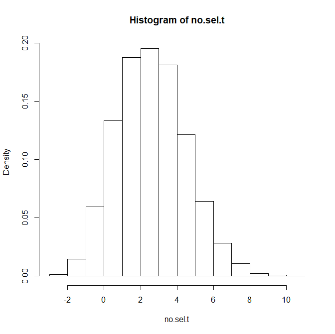
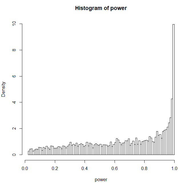
On the blog, Uri Simonsohn shows the Figure below which was based on an example that I provided during our email exchange. The Figure shows the simulated distribution of true power. It also shows the the mean true power is 61%, whereas the p-curve estimate is 79%. Uri Simonssohn does not show the z-curve estimate. He also does not show what the distribution of observed t-values looks like. This is important because few readers are familiar with histograms of power and the fact that it is normal for power to pile up at 1 because 1 is the upper limit for power.

I used the R-Code posted on the Datacolada website to provide additional information about this example. Before I show the results it is important to point out that Uri Simonshon works with a different selection model than Jerry and I. We verified that this has no implications for the performance of p-curve or z-curve, but it does have implications for the distribution of true power that we would expect in real data.
Selection for Significance 1: Jerry and I work with a simple model where researchers conduct studies, test for significance, and then publish the significant results. They may also publish the non-significant results, but they cannot be used to claim a discovery (of course, we can debate whether a significant result implies a discovery, but that is irrelevant here). We use z-curve to estimate the average power of those studies that produced a significant result. As power is the probabilty of obtaining a significant result, the average true power of significant results predicts the success rate in a set of exact replication studies. Therefore, we call this estimate an estimate of replicability.
Selection for Significance 2: The Datacolada team famously coined the term p-hacking. p-hacking refers to massive use of questionable research practices in order to produce statistically significant results. In an influential article, they created the impression that p-hacking allows researchers to get statistical significance in pretty much every study without a real effect (i.e., a false positive). If this were the case, researchers would not have failed studies hidden away like our selection model implies.
No File Drawers: Another Unsupported Claim by Datacolada
In the 2018 volume of Annual Review of Psychology (edited by Susan Fiske), the Datacolada team explicitly claims that psychology researchers do not have file drawers of failed studies.
There is an old, popular, and simple explanation for this paradox. Experiments that work are sent to a journal, whereas experiments that fail are sent to the file drawer (Rosenthal 1979). We believe that this “file-drawer explanation” is incorrect. Most failed studies are not missing. They are published in our journals, masquerading as successes.
They provide no evidence for this claim and ignore evidence to the contrary. For example, Bem (2011) pointed out that it is a common practice in experimental social psychology to conduct small studies so that failed studies can be dismissed as “pilot studies.” In addition, some famous social psychologists have stated explicitly that they have a file drawer of studies that did not work.
“We did run multiple studies, some of which did not work, and some of which worked better than others. You may think that not reporting the less successful studies is wrong, but that is how the field works.” (Roy Baumeister, personal email communication)
In response to replication failures, Kathleen Vohs acknowledged that a couple of studies with non-significant results were excluded from the manuscript submitted for publication that was published with only significant results.
(2) With regard to unreported studies, the authors conducted two additional money priming studies that showed no effects, the details of which were shared with us.
(quote from Rohrer et al., 2015, who failed to replicate Vohs’s findings; see also Vadillo et al., 2016.)
Dan Gilbert and Timothy Wilson acknowledged that they did not publish non-significant results that they considered to be uninformative.
“First, it’s important to be clear about what “publication bias” means. It doesn’t mean that anyone did anything wrong, improper, misleading, unethical, inappropriate, or illegal. Rather it refers to the wellknown fact that scientists in every field publish studies whose results tell them something interesting about the world, and don’t publish studies whose results tell them nothing. Let us be clear: We did not run the same study over and over again until it yielded significant results and then report only the study that “worked.” Doing so would be clearly unethical. Instead, like most researchers who are developing new methods, we did some preliminary studies that used different stimuli and different procedures and that showed no interesting effects. Why didn’t these studies show interesting effects? We’ll never know. Failed studies are often (though not always) inconclusive, which is why they are often (but not always) unpublishable. So yes, we had to mess around for a while to establish a paradigm that was sensitive and powerful enough to observe the effects that we had hypothesized.” (Gilbert and Wilson).
Bias analyses show some problems with the evidence for stereotype threat effects. In a radio interview, Michael Inzlicht reported that he had several failed studies that were not submitted for publication and he is now skeptical about the entirely stereotype threat literature (conflict of interest: Mickey Inzlicht is a friend and colleague of mine who remains the only social psychologists who has published a critical self-analysis of his work before 2011 and is actively involved in reforming research practices in social psychology).
Steve Spencer also acknowledged that he has a file drawer with unsuccessful studies. In 2016, he promised to open his file-drawer and make the results available.
By the end of the year, I will certainly make my whole file drawer available for any one who wants to see it. Despite disagreeing with some of the specifics of what Uli says and certainly with his tone I would welcome everyone else who studies stereotype threat to make their whole file drawer available as well.
Nearly two years later, he hasn’t followed through on this promise (how big can it be? LOL).
Although this anecdotal evidence makes it clear that researchers have file drawers with non-significant results, it remains unclear how large file-drawers are and how often researchers p-hacked null-effects to significance (creating false positive results).
The Influence of Z-Curve on the Distribution of True Power and Observed Test-Statistics
Z-Curve, but not p-curve, can address this question to some extent because p-hacking influences the probability that a low-powered study will be published. A simple selection model with alpha = .05 implies that only 1 out of 20 false positive results produces a significant result and will be included in the set of studies with significant results. In contrast, extreme p-hacking implies that every false positive result (20 out of 20) will be included in the set of studies with significant results.
To illustrate the implications of selection for significance versus p-hacking, it is instructive to examine the distribution of observed significant results based on the simulated distribution of true power in Figure 1.
Figure 2 shows the distribution assuming that all studies will be p-hacked to significance. P-hacking can influence the observed distribution, but I am assuming a simple p-hacking model that is statistically equivalent to optional stopping with small samples. Just keep repeating the experiment (with minor variations that do not influence power to deceive yourself that you are not p-hacking) and stop when you have a significant result.

The histogram of t-values looks very similar to a z-score because t-values with df = 98 are approximately normally distributed. As all studies were p-hacked, all studies are significant with qt(.975,98) = 1.98 as criterion value. However, some studies have strong evidence against the null-hypothesis with t-values greater than 6. The huge pile of t-values just above the criterion value of 1.98 occurs because all low powered studies became significant.
The distribution in Figure 3 looks different than the distribution in Figure 2.
Now there are numerous non-significant results and even a few significant results with the opposite sign of the true effect (t < -1.98). For the estimation of replicability only the results that reached significance are relevant, if only for the reason that they are the only results that are published (success rates in psychology are above 90%; Sterling, 1959, see also real data later on). To compare the distributions it is more instructive to select only the significant results in Figure 3 and to compare the densities in Figures 2 and 3.
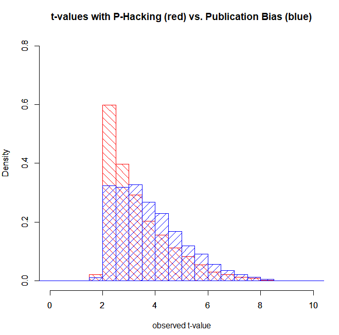
The graph in Figure 4 shows that p-hacking results in more just significant results with t-values between 2 and 2.5 than mere publication bias does. The reason is that the significance filter of alpha = .05 eliminates false positives and low powered true effects. As a result the true power of studies that produced significant results is higher in the set of studies that were selected for significance. The average true power of the honest significant results without p-hacking is 80% (as seen in Figure 1, the average power for the p-hacked studies in red is 61%).
With real data, the distribution of true power is unknown. Thus, it is unknown how much p-hacking occurred. For the reader of a journal that reports only significant it is also irrelevant whether p-hacking occurred. A result may be reported because 10 similar studies tested a single hypothesis or 10 conceptual replication studies produced 1 significant result. In either scenario, the reported significant result provides weak evidence for an effect if the significant result occurred with low power.
It is also important to realize (and it took Jerry and I some time to convince ourselves with simulations that this is actually true) that p-curve and z-curve estimates do not depend on the selection mechanism. The only information that matters is the true power of studies and not how studies were selected. To illustrate this fact, I also used p-curve and z-curve to estimate the average power of the t-values without p-hacking (blue distribution in Figure 4). P-Curve again overestimates true power. While average true power is 80%, the p-curve estimate is 94%.
In conclusion, the datacolada blog post did present one out of several examples that I provided and that were included in the manuscript that I shared with Uri. The Datacolada post correctly showed that z-curve provides good estimates of the average true power and that p-curve produces inflated estimates.
I elaborated on this example by pointing out the distinction between p-hacking (all studies are significant) and selection for significance (e.g., due to publication bias or in assessing replicability of published results). I showed that z-curve produces the correct estimates with and without p-hacking because the selection process does not matter. The only consequence of p-hacking is that more low-powered studies become significant because it undermines the function of the significance filter to prevent studies with weak evidence from entering the literature.
In conclusion, the actual blog post shows that p-curve can be severely biased when data are heterogeneous, which contradicts the title that P-Curve handles heterogeneity just fine.
When The Shoe Doesn’t Fit, Cut of Your Toes
To rescue p-curve and to justify the title, Uri Simonsohn suggests that the example that I provided is unrealistic and that p-curve performs as well or better in simulations that are more realistic. He does not mention that I also provided real world examples in my article that showed better performance of z-curve with real data.
So, the real issue is not whether p-curve handles heterogeneity well (it does not). The real issue is now how much heterogeneity we should expect.
Figure 5 shows that Uri Simonsohn considers to be realistic data. The distribution of true power uses the same beta distribution as the distribution in Figure 1, but instead of scaling it from the lowest possible value (alpha = 5%) to the highest possible value 1-1/infinity), it scales power from alpha to a maximum of 80%. For readers less familiar with power, a value of 80% implies that researches plan studies deliberately with the risk of a 20% probability to end up with a false negative result (i.e., the effect exists, but the evidence is not strong enough, p > .05).
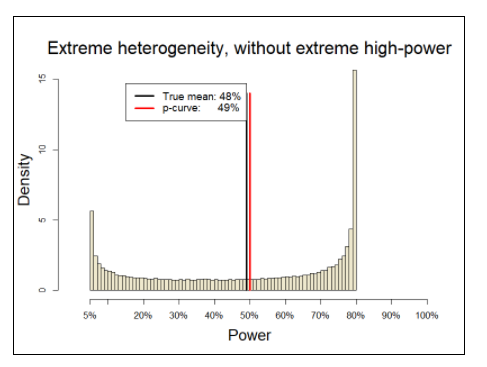
The labeling in the graph implies that studies with more than recommended 80% power, including 81% power are considered to have extremely high power (again, with a 20% risk of a false positive result). The graph also shows that p-curve provided an unbiased estimate of true average power despite (extreme) heterogeneity in true power between 5% and 80%.
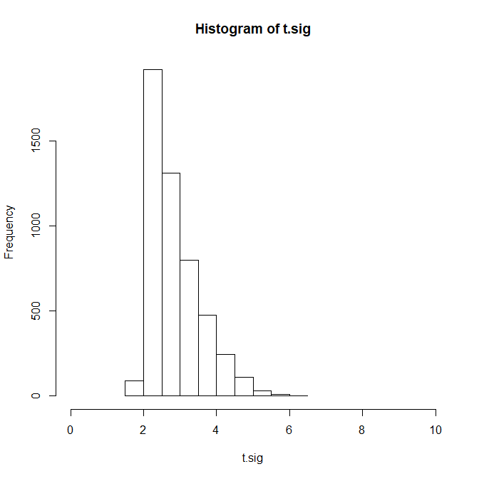
Figure 6 shows the histogram of observed t-values based on a simulation in which all studies in Figure 5 are p-hacked to get significance. As p-hacking inflates all t-values to meet the minimum value of 1.98, and truncation of power to values below 80% removes high t-values, 92% of t-values are within the limited range from 1.98 to 4. A crud measure of heterogeneity is the variance of t-values, which is 0.51. With N = 100, a t-distribution is just a little bit wider than the standard normal distribution, which has a standard deviation of 1. Thus, the small variance of 0.51 indicates that these data have low variability.
The histogram of observed t-values and the variance in these observed t-values makes it possible to quantify heterogeneity in true power. In Figure 2, heterogeneity was high (Var(t) = 1.56) and p-curve overestimated average true power. In Figure 6, heterogeneity is low (Var(t) = 0.51) and p-curve provided accurate estimates. This finding suggests that estimation bias in p-curve is linked to the distribution and variance in observed t-values, which reflects the distribution and variance in true power.
When the data are not simulated, test statistics can come from different tests with different degrees of freedom. In this case, it is necessary to convert all test statistics into z-scores so that strength of evidence is measured in a common metric. In our manuscript, we used the variance of z-scores to quantify heterogeneity and showed that p-curve overestimates when heterogeneity is high.
In conclusion, Uri Simonsohn demonstrated that p-curve can produce accurate estimates when the range of true power is arbitrarily limited to values below 80% power. He suggests that this is reasonable because having more than 80% power is extremely high power and rare.
Thus, there is no disagreement between Uri Simonsohn and us when it comes to the statistical performance of p-curve and z-curve. P-curve overestimates when power is not truncated at 80%. The only disagreement concerns the amount of actual variability in real data.
What is realistic?
Jerry and I are both big fans of Jacob Cohen who has made invaluable contributions to psychology as a science, including his attempt to introduce psychologists to Neyman-Pearson’s approach to statistical inferences that avoids many of the problems of Fishers’ approach that dominates statistics training in psychology to this day.
The concept of statistical power requires that researchers formulate an alternative hypothesis, which requires specifying an expected effect size. To facilitate this task, Cohen developed standardized effect sizes. For example, Cohen’s standardizes a mean difference (e.g., height difference between men and women in centimeters) by the standard deviation. As a result, the effect size is independent of the unit of measurement and is expressed in terms of percentages of a standard deviation. Cohen provided rough guidelines about the size of effect sizes that one could expect in psychology.
It is now widely accepted that most effect sizes are in the range between 0 and 1 standard deviation. It is common to refer to effect sizes of d = .2 (20% of a standard deviation) as small, d = .5 as medium, and d = .8 as large.
True power is a function of effect size and sampling error. In a between subject study sampling error is a function of sample size and most sample sizes in between-subject designs fall into a range from 40 to 200 participants, although sample sizes have been increasing somewhat in response to the replication crisis. With N = 40 to 200, sampling error ranges from 0.14 (2/sqrt(200) to .32 (2/sqrt(40).
The non-central t-values are simply the ratio of standardized effect sizes and sampling error of standardized measures. At the lowest end, effect sizes of 0 have a non-central t-value of 0 (0/.14 = 0; 0/.32 = 0). At the upper end, a large effect size of .8 obtained in the largest sample (N = 200) yields a t-value of .8/.14 = 5.71. While smaller non-central t-values than 0 are not possible, larger non-central t-values can occur in some studies. Either the effect size is very large or sampling error is smaller. Smaller sampling errors are especially likely when studies use covariates, within-subject designs or one-sample t-tests. For example, a moderate effect size (d = .5) in a within-subject design with 90% fixed error variance (r = .9), yields a non-central t-value of 11.
A simple way to simulate data that are consistent with these well-known properties of results in psychology is to assume that the average effect size is half a standard deviation (d = .5) and to model variability in true effect sizes with a normal distribution with a standard deviation of SD = .2. Accordingly, 95% of effect sizes would fall into the range from d = .1 to d = .9. Sample sizes can be modeled with a simple uniform distribution (equal probability) from N = 40 to 200.

Converting the non-centrality parameters to power with p < .05 shows that many values fall into the region from .80 to 1 that Uri Simonsohn called extremely high power. The graph shows that it does not require extremely large effect sizes (d > 1) or large samples (N > 200) to conduct studies with 80% power or more. Of course, the percentage of studies with 80% power or more depends on the distribution of effect sizes, but it seems questionable to assume that studies rarely have 80% power.
The mean true power is 66% (I guess you see where this is going).
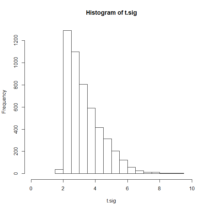
This is the distribution of the observed t-values. The variance is 1.21 and 23% of the t-values are greater than 4. The z-curve estimate is 66% and the p-curve estimate is 83%.
In conclusion, a simulation that starts with knowledge about effect sizes and sample sizes in psychological research shows that it is misleading to call 80% power or more extremely high power that is rarely achieved in actual studies. It is likely that real datasets will include studies with more than 80% power and that this will lead p-curve to overestimate average power.
A comparison of P-Curve and Z-Curve with Real Data
The point of fitting p-curve and z-curve to real data is not to validate the methods. The methods have been validated in simulation studies that show good performance of z-curve and poor performance of p-curve when hterogeneity is high.
The only question remains how biased p-curve is with real data. Of course, this depends on the nature of the data. It is therefore important to remember that the Datacolada team proposed p-curve as an alternative to Cohen’s (1962) seminal study of power in the 1960 issue of the Journal of Abnormal and Social Psychology.
“Estimating the publication-bias corrected estimate of the average power of a set of studies can be useful for at least two purposes. First, many scientists are intrinsically
interested in assessing the statistical power of published research (see e.g., Button et al., 2013; Cohen, 1962; Rossi, 1990; Sedlmeier & Gigerenzer, 1989).
There have been two recent attempts at estimating the replicability of results in psychology. One project conducted 100 actual replication studies (Open Science Collaboration, 2015). A more recent project examined the replicability of social psychology using a larger set of studies and statistical methods to assess replicability (Motyl et al., 2017).
The authors sampled articles from four journals, the Journal of Personality and Social Psychology, Personality and Social Psychology Bulletin, Journal of Experimental Psychology, and Psychological Science and four years, 2003, 2004, 2013, and 2014. They randomly sampled 543 articles that contained 1,505 studies. For each study, a coding team picked one statistical test that tested the main hypothesis. The authors converted test-statistics into z-scores and showed histograms for the years 2003-2004 and 2013-2014 to examine changes over time. The results were similar.
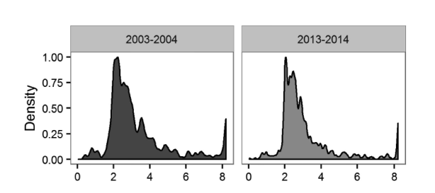
The histograms show clear evidence that non-significant results are missing either due to p-hacking or publication bias. The authors did not use p-curve or z-curve to estimate the average true power. I used these data to examine the performance of z-curve and p-curve. I selected only tests that were coded as ANOVAs (k = 751) or t-tests (k = 232). Furthermore, I excluded cases with very large test statistics (> 100) and experimenter degrees of freedom (10 or more). For participant degrees of freedom, I excluded values below 10 and above 1000. This left 889 test statistics. The test statistics were converted into z-scores. The variance of the significant z-scores was 2.56. However, this is due to a long tail of z-scores with a maximum value of 18.02. The variance of z-scores between 1.96 and 6 was 0.83.
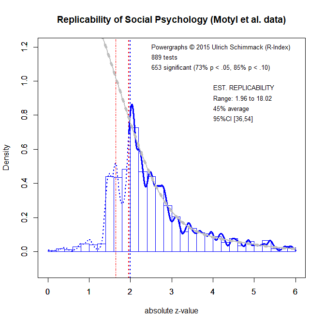
Fitting z-curve to all significant z-scores yielded an estimate of 45% average true power. The p-curve estimate was 78% (90%CI = 75;81). This finding is not surprising given the simulation results and the variance in the Motyl et al. data.
One possible solution to this problem could be to modify p-curve in the same way that z-curve only models z-scores between 1.96 and 6 and treats all z-scores of 6 as having power = 1. The z-curve estimate is then adjusted by the proportion of extreme z-scores
average.true.power = z-curve.estimate * (1 – extreme) + extreme
Using the same approach with p-curve does help to reduce the bias in p-curve estimates, but p-curve still produces a much higher estimate than z-curve, namely 63% (90%CI = .58;67. This is still nearly 20% higher than the z-curve estimate.
In response to these results, Leif Nelson argued that the problem is not with p-curve, but with the Motyl et al. data.
They attempt to demonstrate the validity of the Z-curve with three sets of clearly invalid data.
One of these “clearly invalid” data are the data from Motyl et al.’s study. Nelson claim is based on another datacolada blog post about the Motyl et al. study with the title
[60] Forthcoming in JPSP: A Non-Diagnostic Audit of Psychological Research
A detailed examination of datacolada 60 will be the subject of another open discussion about Datacolada. Here it is sufficient to point that Nelson’s strong claim that Motyl et al.’s data are “clearly invalid” is not based on empirical evidence. It is based on disagreement about the coding of 10 out of over 1,500 tests (0.67%). Moreover, it is wrong to label these disagreements mistakes because there is no right or wrong way to pick one test from a set of tests.
In conclusion, the Datacolada team has provided no evidence to support their claim that my simulations are unrealistic. In contrast, I have demonstrated that their truncated simulation does not match reality. Their only defense is now that I cheery-picked data that make z-curve look good. However, a simulation with realistic assumptions about effect sizes and sample sizes also shows large heterogeneity and p-curve fails to provide reasonable estimates.
The fact that sometimes p-curve is not biased is not particularly important because z-curve provides practically useful estimates in these scenarios as well. So, the choice is between one method that gets it right sometimes and another method that gets it right all the time. Which method would you choose?
It is important to point out that z-curve shows some small systematic bias in some situations. The bias is typically about 2% points. We developed a conservative 95%CI to address this problem and demonstrated that his 95% confidence interval has good coverage under these conditions and is conservative in situations when z-curve is unbiased. The good performance of z-curve is the result of several years of development. Not surprisingly, it works better than a method that has never been subjected to stress-tests by the developers.
Future Directions
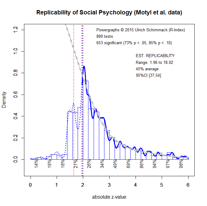
Z-curve has many additional advantages over p-curve. First, z-curve is a model for heterogeneous data. As a result, it is possible to develop methods that can quantify the amount of variability in power while correcting for selection bias. Second, heterogeneity implies that power varies across studies. As studies with higher power tend to produce larger z-scores, it is possible to provide corrected power estimates for sets of z-values. For example, the average power of just significant results (z < 2.5) could be very low.
Although these new features are still under development, first tests show promising results. For example, the local power estimates for Motyl et al. suggest that test statistics with z-scores below 2.5 (p = .012) have only 26% power and even those between 2.5 and 3.0 (p = .0026) have only 34% power. Moreover, test statistics between 1.96 and 3 account for two-thirds of all test statistics. This suggests that many published results in social psychology will be difficult to replicate.
The problem with fixed-effect models like p-curve is that the average may be falsely generalized to individual studies. Accordingly, an average estimate of 45% might be misinterpreted as evidence that most findings are replicable and that replication studies with a little bit power would be able to replicate most findings. However, this is not the case (OSC, 2015). In reality, there are many studies with low power that are difficult to replicate and relatively few studies with very high power that are easy to replicate. Averaging across these studies gives the wrong impression that all studies have moderate power. Thus, p-curve estimates may be misinterpreted easily because p-curve ignores heterogeneity in true power.
Final Conclusion
In the datacolada 67 blog post, the Datacolada team tried to defend p-curve against evidence that p-curve fails when data are heterogeneous. It is understandable that authors are defensive about their methods. In this comment on the blog post, I tried to reveal flaws in Uri’s arguments and to show that z-curve is indeed a better tool for the job. However, I am just as motivated to promote z-curve as the Datacolada team is to promote p-curve.
To address this problem of conflict of interest and motivated reasoning, it is time for third parties to weigh in. Neither method has been vetted by traditional peer-review because editors didn’t see any merit in p-curve or z-curve, but these methods are already being used to make claims about replicability. It is time to make sure that they are used properly. So, please contribute to the discussion about p-curve and z-curve in the comments section. Even if you simply have a clarification question, please post it.