Is there still something new to say about p-values? Yes, there is. Most discussions of p-values focus on a scenario where a researcher tests a new hypothesis computes a p-value and now has to interpret the result. The status quo follows Fisher’s – 100 year old – approach to compare the p-value to a value of .05. If the p-value is below .05 (two-sided), the inference is that the population effect size deviates from zero in the same direction as the observed effect in the sample. If the p-value is greater than .05 the results are deemed inconclusive.

This approach to the interpretation of the data assumes that we have no other information about our hypothesis or that we do not trust this information sufficiently to incorporate it in our inference about the population effect size. Over the past decade, Bayesian psychologists have argued that we should replace p-values with Bayes-Factors. The advantage of Bayes-Factors is that they can incorporate prior information to draw inferences from data. However, if no prior information is available, the use of Bayesian statistics may cause more harm than good. To use priors without prior information, Bayes-Factors are computed with generic, default priors that are not based on any information about a research question. Along with other problems of Bayes-Factors, this is not an appealing solution to the problem of p-values.

Here I introduce a new approach to the interpretation of p-values that has been called empirical Bayesian and has been successfully applied in genomics to control the field-wise false positive rate. That is, prior information does not rest on theoretical assumptions or default values, but rather on prior empirical information. The information that is used to interpret a new p-value is the distribution of prior p-values.

P-value distributions

Every study is a new study because it relies on a new sample of participants that produces sampling error that is independent of the previous studies. However, studies are not independent in other characteristics. A researcher who conducted a study with N = 40 participants is likely to have used similar sample sizes in previous studies. And a researcher who used N = 200 is also likely to have used larger sample sizes in previous studies. Researchers are also likely to use similar designs. Social psychologists, for example, prefer between-subject designs to better deceive their participants. Cognitive psychologists care less about deception and study simple behaviors that can be repeated hundreds of times within an hour. Thus, researchers who used a between-subject design are likely to have used a between-subject design in previous studies and researchers who used a within-subject design are likely to have used a within-subject design before. Researchers may also be chasing different effect sizes. Finally, researchers can differ in their willingness to take risks. Some may only test hypotheses that are derived from prior theories that have a high probability of being correct, whereas others may be willing to shoot for the moon. All of these consistent differences between researchers (i.e., sample size, effect size, research design) influence the unconditional statistical power of their studies, which is defined as the long-run probability of obtaining significant results, p < .05.

Over the past decade, in the wake of the replication crisis, interest in the distribution of p-values has increased dramatically. For example, one approach uses the distribution of significant p-values, which is known as p-curve analysis (Simonsohn et al., 2014). If p-values were obtained with questionable research practices when the null-hypothesis is true (p-hacking), the distribution of significant p-values is flat. Thus, if the distribution is monotonically decreasing from 0 to .05, the data have evidential value. Although p-curve analyses has been extended to estimate statistical power, simulation studies show that the p-curve algorithm is systematically biased when power varies across studies (Bartos & Schimmack, 2020; Brunner & Schimmack, 2020).

As shown in simulation studies, a better way to estimate power is z-curve (Bartos & Schimmack, 2020; Brunner & Schimmack, 2020). Here I show how z-curve analyses of prior p-values can be used to demonstrate that p-values from one researcher are not equal to p-values of other researchers when we take their prior research practices into account. By using this prior information, we can adjust the alpha level of individual researchers to take their research practices into account. To illustrate this use of z-curve, I first start with an illustration how different research practices influence p-value distributions.

Scenario 1: P-hacking

In the first scenario, we assume that a researcher only tests false hypotheses (i.e., the null-hypothesis is always true (Bem, 2011; Simonsohn et al., 2011). In theory, it would be easy to spot false positives because replication studies would produce produce 19 non-significant results for every significant one and significant ones would have different signs. However, questionable research practices lead to a pattern of results where only significant results in one direction are reported, which is the norm in psychology (Sterling, 1959, Sterling et al., 1995; Schimmack, 2012).

In a z-curve analysis, p-values are first converted into z-scores, z = -qnorm(p/2) with qnorm being the inverse normal function and p being a two-sided p-value. A z-curve plot shows the histogram of all z-scores, including non-significant ones (Figure 1).

Visual inspection of the z-curve plot shows that all 200 p-values are significant (on the right side of the criterion value z = 1.96). it also shows that the mode of the distribution as at the significance criterion. Most important, visual inspection shows a steep drop from the mode to the range of non-significant values. That is, while z = 1.96 is the most common value, z = 1.95 is never observed. This drop provides direct visual information that questionable research practices were used because normal sampling error cannot produce such dramatic changes in the distribution.

I am skipping the technical details how the z-curve model is fitted to the distribution of z-scores (Bartos & Schimmack, 2020). It is sufficient to know that the model is fitted to the distribution of significant z-scores with a limited number of model parameters that are equally spaced over the range of z-scores from 0 to 6 (7 parameters, z = 0, z = 1, z = 2, …. z = 6). The model gives different weights to these parameters to match the observed distribution. Based on these estimates, z-curve.2.0 computes several statistics that can be used to interpret single p-values that have been published or future p-values by the same researcher, assuming that the same research practices are used.

The most important statistic is the expected discovery rate (EDR), which corresponds to the average power of all studies that were conducted by a researcher. Importantly, the EDR is an estimate that is based on only the significant results, but makes predictions about the number of non-significant results. In this example with N = 200 participants, the EDR is 7%. Of course, we know that it really is only 5% because the expected discovery rate for true hypotheses that are tested with alpha = .05 is 5%. However, sampling error can introduce biases in our estimates. Nevertheless, even with only 200 observations, the estimate of 7% is relatively close to 5%. Thus, z-curve tells us something important about the way these p-values were obtained. They were obtained in studies with very low power that is close to the criterion value for a false positive result.

Z-curve uses bootstrap to compute confidence intervals around the point estimate of the EDR. the 95%CI ranges from 5% to 18%. As the interval includes 5%, we cannot reject the hypothesis that all tests were false positives (which in this scenario is also the correct conclusion). At the upper end we can see that mean power is low, even if some true hypotheses are being tested.

The EDR can be used for two purposes. First, it can be used to examine the extent of selection for significance by comparing the EDR to the observed discovery rate (ODR; Schimmack, 2012). The ODR is simply the percentage of significant results that was observed in the sample of p-values. In this case, this is 200 out of 200 or 100%. The discrepancy between the EDR of 7% and 100% is large and 100% is clearly outside the 95%CI of the EDR. Thus, we have strong evidence that questionable research practices were used, which we know to be true in this simulation because the 200 tests were selected from a much larger sample of 4,000 tests.

Most important for the use of z-curve to interpret p-values is the ability to estimate the maximum False Discovery Rate (Soric, 1989). The false discovery rate is the percentage of significant results that are false positives or type-I errors. The false discovery rate is often confused with alpha, the long-run probability of making a type-I error. The significance criterion ensures that no more than 5% of significant and non-significant results are false positives. When we test 4,000 false hypotheses (i.e., the null-hypothesis is true) were are not going to have more than 5% (4,000 * .05 = 200) false positive results. This is true in general and it is true in this example. However, when only significant results are published, it is easy to make the mistake to assume that no more than 5% of the published 200 results are false positives. This would be wrong because the 200 were selected to be significant and they are all false positives.

The false discovery rate is the percentage of significant results that are false positives. It no longer matters whether non-significant results are published or not. We are only concerned with the population of p-values that are below .05 (z > 1.96). In our example, the question is how many of the 200 significant results could be false positives. Soric (1989 demonstrated that the EDR limits the number of false positive discoveries. The more discoveries there are, the lower is the risk that discoveries are false. Using a simple formula, we can compute the maximum false discovery rate from the EDR.

FDR = (1/(EDR – 1)*(.05/.95), with alpha = .05

With an EDR of 7%, we obtained a maximum FDR of 68%. We know that the true FDR is 100%, thus, the estimate is too low. However, the reason is that sampling error can have dramatic effects on the FDR estimates when the EDR is low. With an EDR of 6%, the FDR estimate goes up to 82% and with an EDR estimate of 5% it is 100%. To take account of this uncertainty, we can use the 95%CI of the EDR to compute a 95%CI for the FDR estimate, 24% to 100%. Now we see that we cannot rule out that the FDR is 100%.

In short, scenario 1 introduced the use of p-value distributions to provide useful information about the risk that the published results are false discoveries. In this extreme example, we can dismiss the published p-values as inconclusive or as lacking in evidential value.

Scenario 2: The Typical Social Psychologist

It is difficult to estimate the typical effect size in a literature. However, a meta-analysis of meta-analyses suggested that the average effect size in social psychology is Cohen’s d = .4 (Richard et al., 2003). A smaller set of replication studies that did not select for significance estimated an effect size of d = .3 for social psychology (d = .2 for JPSP, d = .4 for Psych Science; Open Science Collaboration, 2015). The later estimate may include an unknown number of hypotheses where the null-hypothesis is true and the true effect size is zero. Thus, I used d = .4 as a reasonable effect size for true hypotheses in social psychology (see also LeBel, Campbell, & Loving, 2017).

It is also known that a rule of thumb in experimental social psychology was to allocate n = 20 participants to a condition, resulting in a sample size of N = 40 in studies with two groups. In a 2 x 2 design, the main effect would be tested with N = 80. However, to keep this scenario simple, I used d = .4 and N = 40 for true effects. This affords 23% power to obtain a significant result.

Finkel, Eastwick, and Reis (2017) argued that power of 25% is optimal if 75% of the hypotheses that are being tested are true. However, the assumption that 75% of hypotheses are true may be on the optimistic side. Wilson and Wixted (2018) suggested that the false discovery risk is closer to 50%. With 23% power for true hypotheses, this implies a false discovery rate of Given uncertainty about the actual false discovery rate in social psychology, I used a scenario with 50% true and 50% false hypotheses.

I kept the number of significant results at 200. To obtain 200 significant results with an equal number of true and false hypotheses, we need 1,428 tests. The 714 true hypotheses contribute 714*.23 = 164 true positives and the 714 false hypotheses produce 714*.05 = 36 false positive results; 164 + 36 = 200. This implies a false discovery rate of 36/200 = 18%. The true EDR is (714*.23+714*.05)/(714+714) = 14%.

The z-curve plot looks very similar to the previous plot, but they are not identical. Although the EDR estimate is higher, it still includes zero. The maximum FDR is well above the actual FDR of 18%, but the 95%CI includes the actual value of 18%.

A notable difference between Figure 1 and Figure 2 is the expected replication rate (ERR), which corresponds to the average power of significant p-values. It is called the estimated replication rate (ERR) because it predicts the percentage of significant results if the studies that were selected for significance were replicated exactly (Brunner & Schimmack, 2020). When power is heterogeneous, power of the studies with significant results is higher than power of studies with non-significant results (Brunner & Schimmack, 2020). In this case, with only two power values, the reason is that false positives have a much lower chance to be significant (5%) than true positives (23%). As a result, the average power of significant studies is higher than the average power of all studies. In this simulation, the true average power of significant studies is the weighted average of true and false positives with significant results, (164*.23 +36*.05)/(164+36) = 20%. Z-curve perfectly estimated this value.

Importantly, the 95% CI of the ERR, 11% to 34%, does not include zero. Thus, we can reject the null-hypotheses that all of the significant results are false positives based on the ERR. In other words, the significant results have evidential value. However, we do not know the composition of this average. It could be a large percentage of false positives and a few true hypotheses with high power or it could be many true positives with low power. We also do not know which of the 200 significant results is a true positive or a false positive. Thus, we would need to conduct replication studies to distinguish between true and false hypotheses. And given the low power, we would only have a 23% chance of successfully replicating a true positive result. This is exactly what happened with the reproducibility project. And the inconsistent results lead to debates and require further replications. Thus, we have real-world evidence how uninformative p-values are when they are obtained this way.

Social psychologists might argue that the use of small samples is justified because most hypotheses in psychology are true. Thus, we can use prior information to assume that significant results are true positives. However, this logic fails when social psychologists test false hypotheses. In this case, the observed distribution of p-values (Figure 1) is not that different from the distribution that is observed when most significant results are true positives that were obtained with low power (Figure 2). Thus, it is doubtful that this is really an optimal use of resources (Finkel et al., 2015). However, until recently this was the way experimental social psychologists conducted their research.

Scenario 3: Cohen’s Way

In 1962 (!), Cohen conducted a meta-analysis of statistical power in social psychology. The main finding was that studies had only a 50% chance to get significant results with a median effect size of d = .5. Cohen (1988) also recommended that researchers should plan studies to have 80% power. However, this recommendation was ignored.

To achieve 80% power with d = .4, researchers need N = 200 participants. Thus, the number of studies is reduced from 5 studies with N = 40 to one study with N = 200. As Finkel et al. (2017) point out, we can make more discoveries with many small studies than a few large ones. However, this ignores that the results of the small studies are difficult to replicate. This was not a concern when social psychologists did not bother to test whether their discoveries are false discoveries or whether they can be replicated. The replication crisis shows the problems of this approach. Now we have results from decades of research that produced significant p-values without providing any information whether these significant results are true or false discoveries.

Scenario 3 examines what social psychology would look like today, if social psychologists had listened to Cohen. The scenario is the same as in the second scenario, including publication bias. There are 50% false hypotheses and 50% true hypotheses with an effect size of d = .4. The only difference is that researchers used N = 200 to test their hypotheses to achieve 80% power.

With 80% power, we need 470 tests (compared to 1,428 in Scenario 2) to produce 200 significant results, 235*.80 + 235*.05 = 188 + 12 = 200. Thus, the EDR is 200/470 = 43%. The true false discovery rate is 6%. The expected replication rate is 188*.80 + 12*.05 = 76%. Thus, we see that higher power increases replicability from 20% to 76% and lowers the false discovery rate from 18% to 6%.

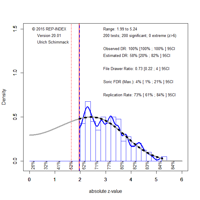
Figure 3 shows the z-curve plot. Visual inspection shows that Figure 3 looks very different from Figures 1 and 2. The estimates are also different. In this example, sampling error inflated the EDR to be 58%, but the 95%CI includes the true value of 46%. The 95%CI does not include the ODR. Thus, there is evidence for publication bias, which is also visible by the steep drop in the distribution at 1.96.

Even with a low EDR of 20%, the maximum FDR is only 21%. Thus, we can conclude with confidence that at least 79% of the significant results are true positives. Remember, in the previous scenario, we could not rule out that most results are false positives. Moreover, the estimated replication rate is 73%, which underestimates the true replication rate of 76%, but the 95%CI includes the true value, 95%CI = 61% – 84%. Thus, if these studies were replicated, we would have a high success rate for actual replication studies.

Just imagine for a moment what social psychology might look like in a parallel universe where social psychologists followed Cohen’s advice. Why didn’t they? The reason is that they did not have z-curve. All they had was p < .05, and using p < .05, all three scenarios are identical. All three scenarios produced 200 significant results. Moreover, as Finkel et al. (2015) pointed out, smaller samples produce 200 significant results quicker than large samples. An additional advantage of small samples is that they inflate point estimates of the population effect size. Thus, the social psychologists with the smallest samples could brag about the biggest (illusory) effect sizes as long as nobody was able to publish replication studies with larger samples that deflated effect sizes of d = .8 to d = .08 (Joy-Gaba & Nosek, 2010).

This game is over, but social psychology – and other social sciences – have published thousands of significant p-values, and nobody knows whether they were obtained using scenario 1, 2, or 3, or probably a combination of these. This is where z-curve can make a difference. P-values are no longer equal when they are considered as a data point from a p-value distribution. In scenario 1, a p-value of .01 and even a p-value of .001 has no meaning. In contrast, in scenario 3 even a p-value of .02 is meaningful and more likely to reflect a true positive than a false positive result. This means that we can use z-curve analyses of published p-values to distinguish between probably false and probably true positives.

I illustrate this with three concrete examples from a project that examined the p-value distributions of over 200 social psychologists (Schimmack, in preparation). The first example has the lowest EDR in the sample. The EDR is 11% and because there are only 210 tests, the 95%CI is wide and includes 5%.

The maximum EDR estimate is high with 41% and the 95%CI includes 100%. This suggests that we cannot rule out the hypothesis that most significant results are false positives. However, the replication rate is 57% and the 95%CI, 45% to 69%, does not include 5%. Thus, some tests tested true hypotheses, but we do not know which ones.

Visual inspection of the plot shows a different distribution than Figure 2. There are more just significant p-values, z = 2.0 to 2.2 and more large z-scores (z > 4). This shows more heterogeneity in power. A comparison of the ODR with the EDR shows that the ODR falls outside the 95%CI of the EDR. This is evidence of publication bias or the use of questionable research practices. One solution to the presence of publication bias is to lower the criterion for statistical significance. As a result, the large number of just significant results is no longer significant and the ODR decreases. This is a post-hoc correction for publication bias. For example, we can lower alpha to .005.

As expected, the ODR decreases considerably from 70% to 39%. In contrast, the EDR increases. The reason is that many questionable research practices produce a pile of just significant p-values. As these values are no longer used to fit the z-curve, it predicts a lot fewer non-significant p-values. The model now underestimates p-values between 2 and 2.2. However, these values do not seem to come from a sampling distribution. Rather they stick out like a tower. By excluding them, the p-values that are still significant with alpha = .005 look more credible. Thus, we can correct for the use of QRPs by lowering alpha and by examining whether these p-values produced interesting discoveries. At the same time, we can ignore the p-values between .05 and .005 and await replication studies to provide empirical evidence whether these hypotheses receive empirical support.

The second example was picked because it was close to the median EDR (33) and ERR (66) in the sample of 200 social psychologists.

The larger sample of tests (k = 1,529) helps to obtain more precise estimates. A comparison of the ODR, 76%, and the 95%CI of the EDR, 12% to 48%, shows that publication bias is present. However, with an EDR of 33%, the maximum FDR is only 11% and the upper limit of the 95%CI is 39%. Thus, we can conclude with confidence that fewer than 50% of the significant results are false positives, however numerous findings might be false positives. Only replication studies can provide this information.

In this example, lowering alpha to .005 did not align the ODR and the EDR. This suggests that these values come from a sampling distribution where non-significant results were not published. Thus, adjusting the there is no simple fix to adjust the significance criterion. In this situation, we can conclude that the published p-values are unlikely to be false positives, but that replication studies are needed to ensure that published significant results are not false positives.

The third example is the social psychologists with the highest EDR. In this case, the EDR is actually a little bit lower than the ODR, suggesting that there is no publication bias. The high EDR also means that the maximum FDR is very small and even the upper limit of the 95%CI is only 7%.

Another advantage of data without publication bias is that it is not necessary to exclude non-significant results from the analysis. Fitting the model to all p-values produces much tighter estimates of the EDR and the maximum FDR.

The upper limit of the 95%CI for the FDR is now 4%. Thus, we conclude that no more than 5% of the p-values less than .05 are false positives. Even p = .02 is unlikely to be a false positive. Finally, the estimated replication rate is 84% with a tight confidence interval ranging from 78% to 90%. Thus, most of the published p-values are expected to replicate in an exact replication study.

I hope these examples make it clear how useful it can be to evaluate single p-values with prior information about the p-values distribution of a lab. As labs differ in their research practices, significant p-values are also different. Only if we ignore the research context and focus on a single result p = .02 equals p = .02. But once we see the broader distribution, p-values of .02 can provide stronger evidence against the null-hypothesis than p-values of .002.

Implications

Cohen tried and failed to change the research culture of social psychologists. Meta-psychological articles have puzzled why meta-analyses of power failed to increase power (Maxwell, 2004; Schimmack, 2012; Sedelmeier & Gigerenzer, 1989). Finkel et al. (2015) provided an explanation. In a game where the winner publishes as many significant results as possible, the optimal strategy is to conduct as many studies as possible with low power. This strategy continues to be rewarded in psychology, where jobs, promotions, grants, and pay raises are based on the number of publications. Cohen (1990) said less is more, but that is not true in a science that does not self-correct and treats every p-value less than .05 as a discovery.

To improve psychology as a science, we need to change the incentive structure and author-wise z-curve analyses can do this. Rather than using p < .05 (or p < .005) as a general rule to claim discoveries, claims of discoveries can be adjusted to the research practices of a researchers. As demonstrated here, this will reward researchers who follow Cohen’s rules and punish those who use questionable practices to produce p-values less than .05 (or Bayes-Factors > 3) without evidential value. And maybe, there is a badge for credible p-values one day.

(incomplete) References

Richard, F. D., Bond, C. F., Jr., & Stokes-Zoota, J. J. (2003). One hundred years of social psychology quantitatively described. Review of General Psychology, 7, 331–363. http://dx.doi.org/10.1037/1089-2680.7.4.331