The statistics wars go back all the way to Fisher, Pearson, and Neyman-Pearson(Jr), and there is no end in sight. I have no illusion that I will be able to end these debates, but at least I can offer a fresh perspective. Lately, statisticians and empirical researchers like me who dabble in statistics have been debating whether p-values should be banned and if they are not banned outright whether they should be compared to a criterion value of .05 or .005 or be chosen on an individual basis. Others have advocated the use of Bayes-Factors.

However, most of these proposals have focused on the traditional approach to test the null-hypothesis that the effect size is zero. Cohen (1994) called this the nil-hypothesis to emphasize that this is only one of many ways to specify the hypothesis that is to be rejected in order to provide evidence for a hypothesis.

For example, a nil-hypothesis is that the difference in the average height of men and women is exactly zero). Many statisticians have pointed out that a precise null-hypothesis is often wrong a priori and that little information is provided by rejecting it. The only way to make nil-hypothesis testing meaningful is to think about the nil-hypothesis as a boundary value that distinguishes two opposing hypothesis. One hypothesis is that men are taller than women and the other is that women are taller than men. When data allow rejecting the nil-hypothesis, the direction of the mean difference in the sample makes it possible to reject one of the two directional hypotheses. That is, if the sample mean height of men is higher than the sample mean height of women, the hypothesis that women are taller than men can be rejected.

However, the use of the nil-hypothesis as a boundary value does not solve another problem of nil-hypothesis testing. Namely, specifying the null-hypothesis as a point value makes it impossible to find evidence for it. That is, we could never show that men and women have the same height or the same intelligence or the same life-satisfaction. The reason is that the population difference will always be different from zero, even if this difference is too small to be practically meaningful. A related problem is that rejecting the nil-hypothesis provides no information about effect sizes. A significant result can be obtained with a large effect size and with a small effect size.

In conclusion, nil-hypothesis testing has a number of problems, and many criticism of null-hypothesis testing are really criticism of nil-hypothesis testing. A simple solution to the problem of nil-hypothesis testing is to change the null-hypothesis by specifying a minimal effect size that makes a finding theoretically or practically useful. Although this effect size can vary from research question to research question, Cohen’s criteria for standardized effect sizes can give some guidance about reasonable values for a minimal effect size. Using the example of mean differences, Cohen considered an effect size of d = .2 small, but meaningful. So, it makes sense to set a criterion for a minimum effect size somewhere between 0 and .2, and d = .1 seems a reasonable value.

We can even apply this criterion retrospectively to published studies with some interesting implications for the interpretation of published results. Shifting the null-hypothesis from d = 0 to d < abs(.1), we are essentially raising the criterion value that a test statistic has to meet in order to be significant. Let me illustrate this first with a simple one-sample t-test with N = 100.

Conveniently, the sampling error for N = 100 is 1/sqrt(100) = .1. To achieve significance with alpha = .05 (two-tailed) and H0:d = 0, the test statistic has to be greater than t.crit = 1.98. However, if we change H0 to d > abs(.1), the t-distribution is now centered at the t-value that is expected for an effect size of d = .1. The criterion value to get significance is now t.crit = 3.01. Thus, some published results that were able to reject the nil-hypothesis would be non-significant when the null-hypothesis specifies a range of values between d = -.1 to .1.

If the null-hypothesis is specified in terms of standardized effect sizes, the critical values vary as a function of sample size. For example, with N = 10 the critical t-value is 2.67, with N = 100 it is 3.01, and with N = 1,000 it is 5.14. An alternative approach is to specify H0 in terms of a fixed test statistic which implies different effect sizes for the boundary value. For example, with t = 2.5, the effect sizes would be d = .06 with N = 10, d = .05 with N = 100, and d = .02 with N = 1000. This makes sense because researchers should use larger samples to test weaker effects. The example also shows that a t-value of 2.5 specifies a very narrow range of values around zero. However, the example was based on one-sample t-tests. For the typical comparison of two groups, a criterion value of 2.5 corresponds to an effect size of d = .1 with N = 100. So, while t = 2.5 is arbitrary, it is a meaningful value to test for statistical significance. With N = 100, t(98) = 2.5 corresponds to an alpha criterion of .014, which is a bit more stringent than .05, but not as strict as a criterion value of .005. With N = 100, alpha = .005 corresponds to a criterion value of t.crit = 2.87, which implies a boundary value of d = .17.

In conclusion, statistical significance depends on the specification of the null-hypothesis. While it is common to specify the null-hypothesis as an effect size of zero, this is neither necessary, nor ideal. An alternative approach is to (re)specify the null-hypothesis in terms of a minimum effect size that makes a finding theoretically interesting or practically important. If the population effect size is below this value, the results could also be used to show that a hypothesis is false. Examination of various effect sizes shows that criterion values in the range between 2 and 3 provide can be used to define reasonable boundary values that vary around a value of d = .1

The problem with t-distributions is that they differ as a function of the degrees of freedom. To create a common metric it is possible to convert t-values into p-values and then to convert the p-values into z-scores. A z-score of 2.5 corresponds to a p-value of .01 (exact .0124) and an effect size of d = .13 with N = 100 in a between-subject design. This seems to be a reasonable criterion value to evaluate statistical significance when the null-hypothesis is defined as a range of smallish values around zero and alpha is .05.

Shifting the significance criterion in this way can dramatically change the evaluation of published results, especially results that are just significant, p < .05 & p > .01. There have been concerns that many of these results have been obtained with questionable research practices that were used to reject the nil-hypothesis. However, these results would not be strong enough to reject the modified hypothesis that the population effect size exceeds a minimum value of theoretical or practical significance. Thus, no debates about the use of questionable research practices are needed. There is also no need to reduce the type-I error rate at the expense of increasing the type-II error rate. It can be simply noted that the evidence is insufficient to reject the hypothesis that the effect size is greater than zero but too small to be important. This would shift any debates towards discussion about effect sizes and proponents of theories would have to make clear which effect sizes they consider to be theoretically important. I believe that this would be more productive than quibbling over alpha levels.

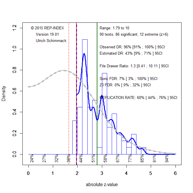
To demonstrate the implications of redefining the null-hypothesis, I use the results of the replicability project (Open Science Collaboration, 2015). The first z-curve shows the traditional analysis for the nil-hypothesis and alpha = .05, which has z = 1.96 as the criterion value for statistical significance (red vertical line).

Figure 1 shows that 86 out of 90 studies reported a test-statistic that exceeded the criterion value of 1.96 for H0:d = 0, alpha = .05 (two-tailed). The other four studies met the criterion for marginal significance (alpha = .10, two-tailed or .05 one-tailed). The figure also shows that the distribution of observed z-scores is not consistent with sampling error. The steep drop at z = 1.96 is inconsistent with random sampling error. A comparison of the observed discovery rate (86/90, 96%) and the expected discovery rate 43% shows evidence that the published results are selected from a larger set of studies/tests with non-significant results. Even the upper limit of the confidence interval around this estimate (71%) is well below the observed discovery rate, showing evidence of publication bias. Z-curve estimates that only 60% of the published results would reproduce a significant result in an actual replication attempt. The actual success rate for these studies was 39%.

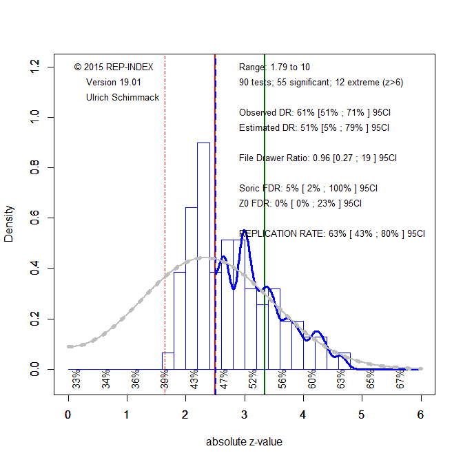
Results look different when the null-hypothesis is changed to correspond to a range of effect sizes around zero that correspond to a criterion value of z = 2.5. Along with shifting the significance criterion, z-curve is also only fitted to studies that produced z-scores greater than 2.5. As questionable research practices have a particularly strong effect on the distribution of just significant results, the new estimates are less influenced by these practices.

Figure 2 shows the results. Most important, the observed discovery rate dropped from 96% to 61%, indicating that many of the original results provided just enough evidence to reject the nil-hypothesis, but not enough evidence to rule out even small effect sizes. The observed discovery rate is also more in line with the expected discovery rate. Thus, some of the missing non-significant results may have been published as just significant results. This is also implied by the greater frequency of results with z-scores between 2 and 2.5 than the model predicts (grey curve). However, the expected replication rate of 63% is still much higher than the actual replication rate with a criterion value of 2.5 (33%). Thus, other factors may contribute to the low success rate in the actual replication studies of the replicability project.

Conclusion

In conclusion, statisticians have been arguing about p-values, significance levels, and Bayes-Factors. Proponents of Bayes-Factors have argued that their approach is supreme because Bayes-Factors can provide evidence for the null-hypothesis. I argue that this is wrong because it is theoretically impossible to demonstrate that a population effect size is exactly zero or any other specific value. A better solution is to specify the null-hypothesis as a range of values that are too small to be meaningful. This makes it theoretically possible to demonstrate that a population effect size is above or below the boundary value. This approach can also be applied retrospectively to published studies. I illustrate this by defining the null-hypothesis as the region of effect sizes that is defined by the effect size that corresponds to a z-score of 2.5. While a z-score of 2.5 corresponds to p = .01 (two-tailed) for the nil-hypothesis, I use this criterion value to maintain an error rate of 5% and to change the null-hypothesis to a range of values around zero that becomes smaller as sample sizes increase.

As p-hacking is often used to just reject the nil-hypothesis, changing the null-hypothesis to a range of values around zero makes many ‘significant’ results non-significant. That is, the evidence is too weak to exclude even trivial effect sizes. This does not mean that the hypothesis is wrong or that original authors did p-hack their data. However, it does mean that they can no longer point to their original results as empirical evidence. Rather they have to conduct new studies to demonstrate with larger samples that they can reject the new null-hypothesis that the predicted effect meets some minimal standard of practical or theoretical significance. With a clear criterion value for significance, authors also risk to obtain evidence that positively contradicts their predictions. Thus, the biggest improvement that arises form rethinking null-hypothesis testing is that authors have to specify effect sizes a priori and that that studies can provide evidence for and against a zero. Thus, changing the nil-hypothesis to a null-hypothesis with a non-null value makes it possible to provide evidence for or against a theory. In contrast, computing Bayes-Factors in favor of the nil-hypothesis fails to achieve this goal because the nil-hypothesis is always wrong, the real question is only how wrong.