When Fisher developed the F-test at Rothamsted Experimental Station in the 1920s, he was solving a real problem. Agricultural field trials had multiple treatment conditions — different fertilizers, different watering regimes, different crop varieties — and the question was whether any of these treatments affected yield. The F-test answered exactly that question: is there more variation between treatments than within them? Any departure from the null was practically interesting because farmers don’t care about direction — they care about which treatment produces the most wheat.
The F-test does this by squaring the differences. The test statistic is always positive. Direction disappears. This is a feature, not a bug, when you have five fertilizers and want to know whether they differ. The omnibus test screens for something worth following up. Fisher then followed up with his Least Significant Difference — ordinary pairwise comparisons gated by the significant F. The omnibus test was a screening step, not the conclusion.
Psychology imported this machinery wholesale, starting in the 1940s. Gigerenzer has told the story of how Fisher’s methods were “cleansed of their agricultural odor” by textbook writers who created the null ritual — mechanical significance testing at p < .05 without specifying alternatives or computing power. But there is a more specific problem that has received less attention: the F-test, by squaring away the sign, trained psychologists to think about hypotheses in unsigned terms. “Is there an effect?” replaced “What is the effect and in which direction?”
This matters less than you might think for multi-group designs, where the omnibus F is doing real work. Testing whether five conditions differ before examining pairwise comparisons is not a ritual — it is a principled gating procedure for multiplicity control. MANOVA before univariate ANOVAs follows the same logic. These are legitimate steps in a testing hierarchy.
But psychology was not mostly running five-group designs. The workhorse experiment had two conditions: treatment versus control. With two groups, F(1, n−2) = t²(n−2). The tests are mathematically identical, but they look different. The t-test has a sign. You can see whether the treatment group scored higher or lower. The F-test strips that away. Psychologists reported F(1, 58) = 4.12, p < .05 when they could have reported t(58) = 2.03, p < .05, and every reader would have immediately seen the direction.
Things got silly. Mark Rubin (2022) argued that it is illegitimate to infer the direction of an effect from a two-sided test — that a significant F or two-sided t only licenses the claim that the means differ, not which is larger. Formally, he is correct that the F-test does not output a direction. But the means are part of the same analysis, and pretending you cannot look at them is a confusion of the test statistic with the inference. Observing that the treatment mean is 12.4 and the control mean is 8.7, and reporting F(1, 58) = 4.12, p < .05, does tell you the treatment increased the outcome. The test confirms the difference is unlikely under the null; the means tell you which way it goes.
This is where the critique of nil-hypothesis testing enters, and where it went partly wrong. Meehl (1967) and Cohen (1994) argued that rejecting the nil hypothesis is scientifically uninformative. They were right that “the means differ somewhere” is a weak conclusion — but this criticism applied most forcefully to the multi-group omnibus F, where Fisher intended it as a screening step. For two-group comparisons, the F-test was always testing a directional effect with the sign obscured.
Here is the point that seems to have been missed. With two groups, a significant F(1, df) at α = .05 is identical to a significant two-sided t(df) at α = .05. And a two-sided test at α = .05 is equivalent to two one-sided tests at α = .025 each. When you reject H₀: μ₁ = μ₂ with a two-sided test and observe that the treatment mean is higher, you have also rejected the directional null H₀: μ₁ ≤ μ₂ at p/2. If you reject μ₁ = μ₂ and observe μ₁ > μ₂, you have rejected μ₁ ≤ μ₂. The sign was always being tested — the F-test just made it invisible.
This means that much of the criticism of NHST — including Gelman and Carlin’s concern about Type S (sign) errors — rests on a misunderstanding. The worry is that a significant result might have the wrong sign, especially in underpowered studies. But a two-sided test that rejects the nil hypothesis does test the sign. The alternative hypothesis is not just “the means differ” — it is partitioned into “the treatment mean is higher” and “the treatment mean is lower,” and the data tell you which one. The sign error problem is real in the sense that underpowered studies can produce unreliable estimates, but it is not a gap in the logic of the test itself. The F-test merely hid this from view.
The real lesson is that statistical tools shape how scientists think. The F-test did not just analyze data — it structured how psychologists formulated hypotheses. By squaring away the sign, it turned every research question into “is there an effect?” rather than “how big, in which direction?” Two generations of methodologists then criticized significance testing for answering a trivial question, when the real problem was that the wrong test statistic was being used for the wrong design. Using t-tests preserves the sign. A positive and significant t-value means the treatment group has a higher mean than the control group, and that this difference is unlikely to have occurred without a real effect. A negative t-value has the opposite implications. Even when the F-test obscures the direction, the observed means still show it, and the significant test licenses the directional inference.
All of these problems dissolve with confidence intervals. A CI that excludes zero and is entirely positive tells you the sign, the magnitude, and the uncertainty in a single object. The F-test, the t-test, and the one-sided versus two-sided debate all become unnecessary.
Andrew Gelman is well known for strong opinions about psychological science, including its methods and research culture (Fiske, 2017. For the most part, he writes as if psychologists are still following a statistical ritual that cannot produce meaningful results. This criticism is not new. It was already made by influential psychologists and methodologists, including Cohen (1990, 1994) and Gigerenzer (2004). The problem with Gelman’s critique is that it is outdated and largely ignores the discussion of null-hypothesis significance testing that took place in psychology during the 1990s. As evidence for this claim, one can simply inspect the reference list of Gelman and Carlin (2014). An article published in Perspectives on Psychological Science does not cite Cohen (1990, 1994), Gigerenzer (2004), or Tukey’s directional reformulation of significance testing (Tukey, 1991; Jones & Tukey, 2000). Although an outsider perspective can be useful for challenging untested assumptions, a commentary that ignores key insights produced by eminent statisticians and methodologists within psychology is unlikely to do so.
The Null-Hypothesis Significance Testing Strawman
As Gigerenzer (2004) pointed out, statistics is often taught as a ritual to be followed rather than as a principled approach to drawing conclusions from data. Rituals are not necessarily bad, but in science it is usually better to understand the rationale and assumptions underlying routine practices.
Null-hypothesis significance testing (NHST) has been described and criticized for decades (Tukey, 1991; Cohen, 1994). Most students of psychology will recognize the following brief description of it. First, researchers collect data that relate one variable to another. Ideally, this is an experiment in which one variable is experimentally manipulated (the independent variable) and the other is observed (the dependent variable). In experiments, a relationship between the independent and dependent variable may justify causal claims, but NHST itself is indifferent to causality. It can be applied to both experimental and correlational data. The main information produced by statistical analyses is the p-value. P-values below a conventional threshold are called statistically significant; those above the threshold are treated as not significant (ns). Significant results are easier to publish. As a result, data analysis often becomes a series of statistical tests searching for statistically significant results (Bem, 2010).
This approach to data analysis has been criticized for several reasons. First, statistical significance by itself does not provide information about effect size. For this reason, psychologists have increasingly reported effect-size estimates in addition to tests of statistical significance, in large part due to Cohen’s (1990) emphasis on effect sizes. Second, NHST has been criticized for its focus on statistically significant findings. Psychology journals have long reported rates of over 90% statistically significant results (Sterling, 1959; Sterling et al., 1995). Publication bias in favor of significant results then leads to inflated effect-size estimates (Rosenthal, 1979).
Most importantly, NHST has been criticized because it appears to reject a null hypothesis that is known to be false before any data are collected. Cohen (1994) called this the nil hypothesis. The nil hypothesis assumes that the population effect size is exactly zero. Statistical significance is then taken to imply that this hypothesis is unlikely to be true and can be rejected. The problem is that rejecting one specific possible effect size tells us very little about the data. It would be equally uninformative to test the hypothesis that the effect size equals any other single value, such as Cohen’s d = .20. So what if the effect size can be said not to be 0 or .20? It could still be 0.01 or 1.99. In short, hypothesis testing with a single point as the null hypothesis is meaningless. Yet that is exactly what psychological articles seem to be reporting when they state p < .05.
What Psychological Scientists Are Implicitly Doing
In reality, however, psychological scientists are doing something different. It may look as if they are testing the nil hypothesis, but in practice they are often testing two directional hypotheses at the same time (Kaiser 1960; Lakens et al., 2025; Tukey, 1991; Jones & Tukey, 2000). When the nil hypothesis is rejected, researchers do not merely conclude that there is a difference. They also inspect the sign of the effect size estimate and infer that the experimental manipulation increased or decreased behavior.
Some authors have argued that drawing directional conclusions from a two-sided test is conceptually problematic (e.g., Rubin, 2020). However, Jones and Tukey explain the rationale for doing so. The easiest way to see this is to reinterpret the standard nil-hypothesis test as two directional tests with two complementary null hypotheses. One null hypothesis states that the effect size is zero or negative. The other states that the effect size is zero or positive. Rejecting the first leads to the inference that the effect is probably positive. Rejecting the second leads to the inference that the effect is probably negative. Viewed this way, zero is simply the boundary between two rejection regions.
Because NHST can be understood in this way as involving two directional possibilities, alpha must be allocated across both tails to maintain the long-run error rate. No psychology student would be surprised to see a t distribution with 2.5% of the area in each tail. Each tail represents the error rate for one directional rejection, and together they produce the familiar two-sided alpha level of 5%.
Most psychology students are not taught that they are implicitly conducting directional tests when they interpret significant p values, but their actual practice shows that this is what they are doing. They routinely draw directional inferences from NHST, and this is a legitimate use of the procedure. It also makes NHST more meaningful than the strawman version in which researchers merely reject an exact value of zero that is often known in advance to be false.
Using NHST to infer the direction of population effects is meaningful because researchers often do not know that direction before data are collected. Empirical data can therefore provide genuinely new information. This is not a full defense of NHST, because effect size and practical importance can still be ignored, but it does show that psychologists have not spent decades and millions of dollars merely to establish that effect sizes are not exactly zero.
Gelman’s Type-S Error
Gelman and Tuerlinckx (2000) criticized NHST because “the significance of comparisons … is calibrated using the Type 1 error rate, relying on the assumption that the true difference is zero, which makes no sense in many applications.” To replace this framework, they proposed focusing on Type S error, where S stands for sign. A Type S error occurs when a researcher makes a confident directional claim even though the true effect has the opposite sign.
The label Type S error is potentially confusing because it suggests a replacement for the Type I error framework rather than a refinement of it. A Type I error is the unconditional long-run probability of falsely rejecting a null hypothesis across all tests that are conducted. For example, suppose a researcher conducts 100 tests with a significance criterion (alpha) of 5%. This criterion ensures that in the long run no more than 5% of all tests will be false positives. Testing at least some real effects will reduce the probability of a false positive. For example, if all studies have high power to detect a true effect, the probability of a false positive is zero (Soric, 1989). Thus, alpha sets a range of the relative frequency of false positives between 0 and alpha.
This unconditional probability must be distinguished from the conditional probability of error among the subset of studies that produced statistically significant results. In the previous example, if only 5 results were significant, it is likely that all 5 rejections were errors and that the conditional probability of a false positive given a significant result is 5 / 5 = 100% (Sorić, 1989). The proportion of false rejections among statistically significant results is called the false discovery rate (FDR), and the estimation and control of FDRs has become a large literature in statistics (Benjamini & Hochberg, 1995).
Applying Jones and Tukey’s interpretation of NHST to false discovery rates, a false discovery occurs not only when the true effect size is zero but also when it is in the opposite direction of the significant result. Gelman’s Type S error rate, also called the false sign rate (Stephens, 2017), assumes that effect sizes are never zero and counts only false rejections with the opposite sign. False sign rates are necessarily smaller than false discovery rates because wrong-sign rejections are only a subset of all false rejections. Exact-zero effects can produce significant results in either direction, whereas nonzero effects make correct-sign rejections more likely and wrong-sign rejections less likely.
The key source of confusion is that Gelman’s criticism of NHST and FDR estimation rests on a misunderstanding of NHST (Gelman, 2021). He maintains that FDR estimates are limited to the unlikely scenario that an effect is exactly zero and ignores sign errors. However, as Jones and Tukey (2000) pointed out, psychological researchers routinely use NHST as a directional sign test. Once NHST is understood in this way, Type S errors are no longer a fundamentally new kind of inferential problem and are already included in conditional and unconditional error rates. Moreover, NHST provides researchers with concrete statistical tools to estimate and control error rates, whereas Gelman’s Type S error is not something that can be estimated and was introduced as a rhetorical tool without practical use (Gelman, 2025; Lakens et al., 2025). In contrast, estimation of false discovery rates and false sign rates is an active area of research in statistics that builds on the foundations of NHST (Benjamini & Hochberg, 1995; Stephens, 2017) and has been largely ignored in psychology.
Statistical Power
So far, the distinction between Type I and (unconditional) Type S errors is mostly harmless. It may even help clarify that NHST is really used as a test of the sign of the population effect size rather than as a literal test of the nil hypothesis (Jones & Tukey, 2000). However, the wheels come off when Gelman and Carlin (2014) extend this critique from Type I error to Type II error and statistical power.
The distinction between Type I and Type II errors was introduced by Neyman and Pearson. A Type II error is the probability of failing to reject a false null hypothesis. Neyman and Pearson were cautious and avoided framing results as inferences about a true effect or as acceptance of a true hypothesis. In practice, however, failure to reject a false hypothesis means that either the population effect is positive and the study failed to produce a statistically significant result with a positive sign, or the population effect is negative and the study failed to produce a statistically significant result with a negative sign.
Statistical power is simply the complementary probability of obtaining a statistically significant result with the correct sign. Unlike the discussion of Type I errors, there is no important distinction here between a point null and an opposite-sign error. Power calculations are inherently directional. Researchers assume either a positive or a negative effect and then choose a design and sample size that reduce sampling error while controlling the Type I error rate. For example, a comparison of two groups with n = 50 per group, a population effect size of half a standard deviation (Cohen’s d = .50), and alpha = .05 has about a 70% probability of producing a statistically significant result with the correct sign.
By definition, then, power already concerns rejections with the correct sign. At this point, there is no meaningful difference between standard NHST and Gelman’s Type S framework (Stephens, 2017). The only minor difference arises in hypothetical scenarios with extremely low power. For two-sided (non-directional) power calculations, low power can produce significant results with sign errors. To use NHST as a sign-test in Jones and Tukey framework of two simultaneous one-sided tests, power should be estimated for one-sided directional tests with alpha/2. However, in practice, this distinction is irrelevant because Gelman and Carlin already showed that even modest power of 50% renders sign errors practically impossible.
Thus, the main concern about Gelman and Carlin’s (2014) article is the false implication that power calculations ignore sign errors and that researchers must move “beyond power” to control them. Grounding NHST in Jones and Tukey’s (2000) framework of two simultaneous directional tests shows that power calculations are not flawed. High power prevents both false negatives and sign errors. Gelman’s critique rests on a false premise: the assumption that NHST is nil-hypothesis testing. Under that assumption, power appears disconnected from sign errors. But once NHST is understood as directional inference, the criticism is invalid. Power analysis is not only useful but essential for controlling sign errors and the false sign rate.
Implications
Here’s a shortened version:
Implications
Gelman positions the Type S error as a new concept that requires moving “beyond power” because “power analysis is flawed” (p. 641). On closer inspection, power analysis is necessary and sufficient to control Type S error rates. Studies with high power ensure that most significant results have the correct sign, and high power also ensures a high discovery rate, which limits the proportion of false discoveries (Sorić, 1989). Power delivers everything needed to make significant results credible. It is paradoxical to criticize psychology for relying on small samples while also criticizing the tool that tells researchers how to avoid them. Cohen’s lasting contribution was precisely this: demonstrating that many studies lack power to detect plausible but small effect sizes and providing the tools to do better (Cohen, 1962).
Gelman and Carlin’s (2014) framing of power as flawed may have added to misunderstandings about the role of power in ensuring credible results. NHST and power analysis are not flawed. They are statistical tools for drawing conclusions about the direction of population effect sizes (Maxwell, Kelley, & Rausch, 2008). It would be desirable to conduct all studies with enough precision to provide informative effect size estimates, but limited resources often make this impossible. Meta-analysis of smaller studies can yield precise estimates, provided results are reported without selection bias. Reporting outcomes regardless of statistical significance is the most effective way to address selection bias, which remains the biggest threat to the credibility of NHST in practice (Sterling, 1959).
The real problem of NHST is not solved by a focus on Type S errors. The real problem is that non-significant results are inconclusive because failure to provide evidence for a positive or negative effect does not allow inferring the absence of an effect (Altman & Bland, 1995). The solution is to distinguish three hypotheses (Rice & Krakauer, 2023): (a) the effect is positive and larger than a smallest effect size of interest, (b) the effect is negative and larger in magnitude than a smallest effect size of interest, and (c) the effect falls within a region of practical equivalence around zero. Evidence for absence is established if the confidence interval falls entirely within the middle region. Replacing the point nil hypothesis with a range of practically equivalent values is an important addition to statistics for psychologists (Lakens, 2017; Lakens, Scheel, & Isager, 2018). It helps distinguish between statistical and practical significance, and it can turn non-significant results into significant evidence for the absence of a meaningful effect. However, providing evidence for absence often requires large samples because precise confidence intervals are needed to fit within a narrow region around zero. Power analysis remains essential for planning studies with this goal.
Conclusion
Continued controversy about NHST shows that better education about its underlying logic is needed. Jones and Tukey (2000) provided a clear explanation that deserves to be foundational for the teaching of NHST. Understanding NHST as two simultaneous directional tests avoids the confusion created by decades of criticism directed at a strawman version of the procedure. NHST has persisted for nearly a century despite harsh criticism because it provides a minimal but useful inference: determining the likely sign of a population effect size. Students need to learn about the real limitations of NHST and how they can be addressed. Changing statistical methods does not solve the problem that researchers need to publish and that precise effect size estimates are often out of reach. Even power to infer the sign of an effect is often low. Honest reporting of a single well-powered study is more important than reporting multiple underpowered studies that are p-hacked or selected for significance (Schimmack, 2012). With good data, different statistical approaches lead to the same conclusion. Open science reforms that improve the quality of data are more important than new statistical methods. The main reason NHST continues to attract criticism is that criticism is easy, but finding a better solution is harder. Real progress requires a real analysis of the problem NHST has many problems, but ignoring sign errors is not one of them.
Ten years ago, a stunning article by Bem (2011) triggered a crisis of confidence about psychology as a science. The article presented nine studies that seemed to show time-reversed causal effects of subliminal stimuli on human behavior. Hardly anybody believed the findings, but everybody wondered how Bem was able to produce significant results for effects that do not exist. This triggered a debate about research practices in social psychology.
Over the past decade, most articles on the replication crisis in social psychology pointed out problems with existing practices, but some articles tried to defend the status quo (cf. Schimmack, 2020).
Finkel, Eastwick, and Reis (2015) contributed to the debate with a plea to balance false positives and false negatives.
I argue that the main argument in this article is deceptive, but before I do so it is important to elaborate a bit on the use of the word deceptive. Psychologists make a distinction between self-deception and other-deception. Other-deception is easy to explain. For example, a politician may spread a lie for self-gain knowing full well that it is a lie. The meaning of self-deception is also relatively clear. Here individuals are spreading false information because they are unaware that the information is false. The main problem for psychologists is to distinguish between self-deception and other-deception. For example, it is unclear whether Donald Trump’s and his followers’ defence mechanisms are so strong that they really believes the election was stolen without any evidence to support this belief or whether he is merely using a lie for political gains. Similarly, it is also unclear whether Finkel et al. were deceiving themselves when they characterized the research practices of relationship researchers as an error-balanced approach, but the distinction between self-deception and other-deception is irrelevant. Self-deception also leads to the spreading of misinformation that needs to be corrected.
In short, my main thesis is that Finkel et al. misrepresent research practices in psychology and that they draw false conclusions about the status quo and the need for change based on a false premise.
Common Research Practices in Psychology
Psychological research practices follow a number of simple steps.
1. Researchers formulate a hypothesis that two variables are related (e.g., height is related to weight; dieting leads to weight loss).
2. They find ways to measure or manipulate a potential causal factor (height, dieting) and find a way to measure the effect (weight).
3. They recruit a sample of participants (e.g., N = 40).
4. They compute a statistic that reflects the strength of the relationship between the two variables (e.g., height and weight correlate r = .5).
5. They determine the amount of sampling error given their sample size.
6. They compute a test-statistic (t-value, F-value, z-score) that reflects the ratio of the effect size over the sample size (e.g., r (40) = .5; t(38) = 3.56.
7. They use the test-statistic to decide whether the relationship in the sample (e.g., r = .5) is strong enough to reject the nil-hypothesis that the relationship in the population is zero (p = .001).
The important question is what researchers do after they compute a p-value. Here critics of the status quo (the evidential value movement) and Finkel et al. make divergent assumptions.
The Evidential Value Movement
The main assumption of the EVM is that psychologists, including relationship researchers, have interpreted p-values incorrectly. For the most part, the use of p-values in psychology follows Fisher’s original suggestion to use a fixed criterion value of .05 to decide whether a result is statistically significant. In our example of a correlation of r = .5 with N = 40 participants, a p-value of .001 is below .05 and therefore it is sufficiently unlikely that the correlation could have emerged by chance if the real correlation between height and weight was zero. We therefore can reject the nil-hypothesis and infer that there is indeed a positive correlation.
However, if a correlation is not significant (e.g., r = .2, p > .05), the results are inconclusive because we cannot infer from a non-significant result that the nil-hypothesis is true. This creates an asymmetry in the value of significant results. Significant results can be used to claim a discovery (a diet produces weight loss), but non-significant results cannot be used to claim that there is no relationship (a diet has no effect on weight).
This asymmetry explains why most published articles results in psychology report significant results (Sterling, 1959; Sterling et al., 1959). As significant results are more conclusive, journals found it more interesting to publish studies with significant results.
As Sterling (1959) pointed out, if only significant results are published, statistical significance no longer provides valuable information, and as Rosenthal (1979) warned, in theory journals could be filled with significant results even if most results are false positives (i.e., the nil-hypothesis is actually true).
Importantly, Fisher did not prescribe to do studies only once and to publish only significant results. Fisher clearly stated that results should only be considered credible if replication studies confirm the original results most of the time (say 8 out of 10 replication studies also produced p < .05). However, this important criterion of credibility was ignored by social psychologists, especially in research areas like relationship research that is resource intensive.
To conclude, the main concern among critics of research practices in psychology is that selective publishing of significant results produces results that have a high risk of being false positives (cf. Schimmack, 2020).
The Error Balanced Approach
Although Finkel et al. (2015) do not mention Neyman and Pearson, their error-balanced approach is rooted in Neyman-Pearsons approach to the interpretation of p-values. This approach is rather different from Fisher’s approach and it is well documented that Fisher and Neyman-Pearson were in a bitter fight over this issue. Neyman and Pearson introduced the distinction between Type I errors also called false positives and type-II errors also called false negatives.
The type-I error is the same error that one could make in Fisher’s approach, namely a significant results, p < .05, is falsely interpreted as evidence for a relationship when there is no relationship between two variables in the population and the observed relationship was produced by sampling error alone.
So, what is a type-II error? It only occurred to me yesterday that most explanations of type-II errors are based on a misunderstanding of Neyman-Pearson’s approach. A simplistic explanation of a type-II error is the inference that there is no relationship, when a relationship actually exists. In the pregnancy example, a type-II error would be a pregnancy test that suggests a pregnant woman is not pregnant.
This explains conceptually what a type-II error is, but it does not explain how psychologists could ever make a type-II error. To actually make type-II errors, researchers would have to approach research entirely differently than psychologists actually do. Most importantly, they would need to specify a theoretically expected effect size. For example, researchers could test the nil-hypothesis that a relationship between height and weight is r = 0 against the alternative hypothesis that the relationship is r = .4. They would then need to compute the probability of obtaining a non-significant result under the assumption that the correlation is r = .4. This probability is known as the type-II error probability (beta). Only then, a non-significant result can be used to reject the alternative hypothesis that the effect size is .4 or larger with a pre-determined error rate beta. If this suddenly sounds very unfamiliar, the reason is that neither training nor published articles follow this approach. Thus, psychologists never make type-II error because they never specify a priori effect sizes and use p-values greater than .05 to infer that population effect sizes are smaller than a specified effect size.
However, psychologists often seem to believe that they are following Neyman-Pearson because statistics is often taught as a convoluted, incoherent mishmash of the two approaches (Gigerenzer, 1993). It also seems that Finkel et al. (2015) falsely assumed that psychologists follow Neyman-Pearson’s approach and carefully weight the risks of type-I and type-II errors. For example, they write
Psychological scientists typically set alpha (the theoretical possibility of a false positive) at .05, and, following Cohen (1988), they frequently set beta (the theoretical possibility of a false negative) at .20.
It is easy to show that this is not the case. To set the probability of a type-II error at 20%, psychologists would need to specify an effect size that gives them an 80% probability (power) to reject the nil-hypothesis, and they would then report the results with the conclusion that the population effect size is less than their a priori specified effect size. I have read more than 1,000 research articles in psychology and I have never seen an article that followed this approach. Moreover, it has been noted repeatedly that sample sizes are determined on an ad hoc basis with little concerns about low statistical power (Cohen, 1962; Sedlmeier & Gigerenzer, 1989; Schimmack, 2012; Sterling et al., 1995). Thus, the claim that psychologists are concerned about beta (type-II errors) is delusional, even if many psychologists believe it.
Finkel et al. (2015) suggests that an optimal approach to research would balance the risk of false positive results with the risk of false negative results. However, once more they ignore that false negatives can only be specified with clearly specified effect sizes.
Estimates of false positive and false negative rates in situations like these would go a long way toward helping scholars who work with large datasets to refine their confirmatory and exploratory hypothesis testing practices to optimize the balance between false-positive and false-negative error rates.
Moreover, they are blissfully unaware that false positive rates are abstract entities because it is practically impossible to verify that the relationship between two variables in a population is exactly zero. Thus, neither false positives nor false negatives are clearly defined and therefore cannot be counted to compute rates of their occurrences.
Without any information about the actual rate of false positives and false negatives, it is of course difficult to say whether current practices produce too many false positives or false negatives. A simple recommendation would be to increase sample sizes because higher statistical power reduces the risk of false negatives and the risk of false positives. So, it might seem like a win-win. However, this is not what Finkel et al. considered to be best practices.
“As discussed previously, many policy changes oriented toward reducing false-positive rates will exacerbate false-negative rates”
This statement is blatantly false and ignores recommendations to test fewer hypotheses in larger samples (Cohen, 1990; Schimmack, 2012).
They further make unsupported claims about the difficulty of correcting false positive results and false negative results. The evidential value critics have pointed out that current research practices in psychology make it practically impossible to correct a false positive result. Classic findings that failed to replicate are often cited and replications are ignored. The reason is that p < .05 is treated as strong evidence, whereas p > .05 is treated as inconclusive, following Fisher’s approach. If p > .05 was considered evidence against a plausible hypothesis, there would be no reason not to publish it (e.g., a diet does not decrease weight by more than .3 standard deviations in a study with 95% power, p < .05).
We are especially concerned about the evidentiary value movement’s relative neglect of false negatives because, for at least two major reasons, false negatives are much less likely to be the subject of replication attempts. First, researchers typically lose interest in unsuccessful ideas, preferring to use their resources on more “productive” lines of research (i.e., those that yield evidence for an effect rather than lack of evidence for an effect). Second, others in the field are unlikely to learn about these failures because null results are rarely published (Greenwald, 1975). As a result, false negatives are unlikely to be corrected by the normal processes of reconsideration and replication. In contrast, false positives appear in the published literature, which means that, under almost all circumstances, they receive more attention than false negatives. Correcting false positive errors is unquestionably desirable, but the consequences of increasingly favoring the detection of false positives relative to the detection of false negatives are more ambiguous.
This passage makes no sense. As the authors themselves acknowledge, the key problem with existing research practices is that non-significant results are rarely published (“because null-results are rarely published”). In combination with low statistical power to detect small effect sizes, this selection implies that researchers will often obtain non-significant results that are not published. However, it also means that published significant results often inflate the effect size because the true population effect size alone is too weak to produce a significant result. Only with the help of sampling error, the observed relationship is strong enough to be significant. So, many correlations that are r = .2 will be published as correlations of r = .5. The risk of false negatives is also reduced by publication bias. Because researchers do not know that a hypothesis was tested and produced a non-significant result, they will try again. Eventually, a study will produce a significant result (green jelly beans cause acne, p < .05), and the effect size estimate will be dramatically inflated. When follow-up studies fail to replicate this finding, these replication results are again not published because non-significant results are considered inconclusive. This means that current research practices in psychology never produce type-II errors, only produce type-I errors, and type-I errors are not corrected. This fundamentally flawed approach to science has created the replication crisis.
In short, while evidential value critics and Finkel agree that statistical significance is widely used to decide editorial decisions, they draw fundamentally different conclusions from this practice. Finkel et al. falsely label non-significant results in small samples, false negative results, but they are not false negatives in Neyman-Pearson’s approach to significance testing. They are, however, inconclusive results and the best practice to avoid inconclusive results would be to increase statistical power and to specify type-II error probabilities for reasonable effect sizes.
Finkel et al. (2015) are less concerned about calls for higher statistical power. They are more concerned with the introduction of badges for materials sharing, data sharing, and preregistration as “quick-and-dirty indicator of which studies, and which scholars, have strong research integrity” (p. 292).
Finkel et al. (2015) might therefore welcome cleaner and more direct indicators of research integrity that my colleagues and I have developed over the past decade that are related to some of their key concerns about false negative and false positive results (Bartos & Schimmack, 2020; Brunner & Schimmack, 2020, Schimmack, 2012; Schimmack, 2020). To illustrate this approach, I am using Eli J. Finkel’s published results.
I first downloaded published articles from major social and personality journals (Schimmack, 2020). I then converted these pdf files into text files and used R-code to find statistical results that were reported in the text. I then used a separate R-code to search these articles for the name “Eli J. Finkel.” I excluded thank you notes. I then selected the subset of test statistics that appeared in publications by Eli J. Finkel. The extracted test statistics are available in the form of an excel file (data). The file contains 1,638 useable test statistics (z-scores between 0 and 100).
A z-curve analysis of test-statistic converts all published test-statistics into p-values. Then the p-values are converted into z-scores on an standard normal distribution. Because the sign of an effect does not matter, all z-scores are positive The higher a z-score, the stronger is the evidence against the null-hypothesis. Z-scores greater than 1.96 (red line in the plot) are significant with the standard criterion of p < .05 (two-tailed). Figure 1 shows a histogram of the z-scores between 0 and 6; 143 z-scores exceed the upper value. They are included in the calculations, but not shown.
The first notable observation in Figure 1 is that the peak (mode) of the distribution is just to the right side of the significance criterion. It is also visible that there are more results just to the right (p < .05) than to the left (p > .05) around the peak. This pattern is common and reflects the well-known tendency for journals to favor significant results.
The advantage of a z-curve analysis is that it is possible to quantify the amount of publication bias. To do so, we can compare the observed discovery rate with the expected discovery rate. The observed discovery rate is simply the percentage of published results that are significant. Finkel published 1,031 significant results, which is a percentage of 63%.
The expected discovery rate is based on a statistical model. The statistical model is fitted to the distribution of significant results. To produce the distribution of significant results in Figure 1, we assume that they were selected from a larger set of tests that produced significant and non-significant results. Based on the mean power of these tests, we can estimate the full distribution before selection for significance. Simulation studies show that these estimates match simulated true values reasonably well (Bartos & Schimmack, 2020).
The expected discovery rate is 26%. This estimate implies that the average power of statistical tests conducted by Finkel is low. With over 1,000 significant test statistics, it is possible to obtain a fairly close confidence interval around this estimate, 95%CI = 11% to 44%. The confidence interval does not include 50%, showing that the average power is below 50%, which is often considered a minimum value for good science (Tversky & Kahneman, 1971). The 95% confidence interval also does not include the observed discovery rate of 63%. This shows the presence of publication bias. These results are by no means unique to Finkel. I was displeased to see that a z-curve analysis of my own articles produced similar results (ODR = 74%, EDR = 25%).
The EDR estimate is not only useful to examine publication bias. It can also be used to estimate the maximum false discovery rate (Soric, 1989). That is, although it is impossible to specify how many published results are false positives, it is possible to quantify the worst case scenario. Finkel’s EDR estimate of 26% implies a maximum false discovery rate of 15%. Once again, this is an estimate and it is useful to compute a confidence interval around it. The 95%CI ranges from 7% to 43%. On the one hand, this makes it possible to reject Ioannidis’ claim that most published results are false. On the other hand, we cannot rule out that some of Finkel’s significant results were false positives. Moreover, given the evidence that publication bias is present, we cannot rule out the possibility that non-significant results that failed to replicate a significant result are missing from the published record.
A major problem for psychologists is the reliance on p-values to evaluate research findings. Some psychologists even falsely assume that p < .05 implies that 95% of significant results are true positives. As we see here, the risk of false positives can be much higher, but significance does not tell us which p-values below .05 are credible. One solution to this problem is to focus on the false discovery rate as a criterion. This approach has been used in genomics to reduce the risk of false positive discoveries. The same approach can also be used to control the risk of false positives in other scientific disciplines (Jager & Leek, 2014).
To reduce the false discovery rate, we need to reduce the criterion to declare a finding a discovery. A team of researchers suggested to lower alpha from .05 to .005 (Benjamin et al. 2017). Figure 2 shows the results if this criterion is used for Finkel’s published results. We now see that the number of significant results is only 579, but that is still a lot of discoveries. We see that the observed discovery rate decreased to 35%. The reason is that many of the just significant results with p-values between .05 and .005 are no longer considered to be significant. We also see that the expected discovery rate increased! This requires some explanation. Figure 2 shows that there is an excess of significant results between .05 and .005. These results are not fitted to the model. The justification for this would be that these results are likely to be obtained with questionable research practices. By disregarding them, the remaining significant results below .005 are more credible and the observed discovery rate is in line with the expected discovery rate.
The results look different if we do not assume that questionable practices were used. In this case, the model can be fitted to all p-values below .05.
If we assume that p-values are simply selected for significance, the decrease of p-values from .05 to .005 implies that there is a large file-drawer of non-significant results and the expected discovery rate with alpha = .005 is only 11%. This translates into a high maximum false discovery rate of 44%, but the 95%CI is wide and ranges from 14% to 100%. In other words, the published significant results provide no credible evidence for the discoveries that were made. It is therefore charitable to attribute the peak of just significant results to questionable research practices so that p-values below .005 provide some empirical support for the claims in Finkel’s articles.
Discussion
Ultimately, science relies on trust. For too long, psychologists have falsely assumed that most if not all significant results are discoveries. Bem’s (2011) article made many psychologists realize that this is not the case, but this awareness created a crisis of confidence. Which significant results are credible and which ones are false positives? Are most published results false positives? During times of uncertainty, cognitive biases can have a strong effect. Some evidential value warriors saw false positive results everywhere. Others wanted to believe that most published results are credible. These extreme positions are not supported by evidence. The reproducibility project showed that some results replicate and others do not (Open Science Collaboration, 2015). To learn from the mistakes of the past, we need solid facts. Z-curve analyses can provide these facts. It can also help to separate more credible p-values from less credible p-values. Here, I showed that about half of Finkel’s discoveries can be salvaged from the wreckage of the replication crisis in social psychology by using p < .005 as a criterion for a discovery.
However, researchers may also have different risk preferences. Maybe some are more willing to build on a questionable, but intriguing finding than others. Z-curve analysis can accommodate personalized risk-preferences as well. I shared the data here and an R-package is available to fit z-curve with different alpha levels and selection thresholds.
Aside from these practical implications, this blog post also made a theoretical observation. The term type-II error or false negative is often used loosely and incorrectly. Until yesterday, I also made this mistake. Finkel et al. (2015) use the term false negative to refer to all non-significant results were the nil-hypothesis is false. They then worry that there is a high risk of false negatives that needs to be counterbalanced against the risk of a false positive. However, not every trivial deviation from zero is meaningful. For example, a diet that reduces weight by 0.1 pounds is not worthwhile studying. A real type-II error is made when researcher specify a meaningful effect size, conduct a high-powered study to find it, and then falsely conclude that an effect of this magnitude does not exist. To make a type-II error, it is necessary to conduct studies with high power. Otherwise, beta is so high that it makes no sense to draw a conclusion from the data. As average power in psychology in general and in Finkel’s studies is low, it is clear that they did not make any type-II errors. Thus, I recommend to increase power to finally get a balance between type-I and type-II errors which requires making some type-II errors some of the time.
References
Gigerenzer, G. (1993). The superego, the ego, and the id in statistical reasoning. In G. Keren & C. Lewis (Eds.), A handbook for data analysis in the behavioral sciences: Methodological issues (pp. 311–339). Hillsdale, NJ: Erlbaum, Inc.
The statistics wars go back all the way to Fisher, Pearson, and Neyman-Pearson(Jr), and there is no end in sight. I have no illusion that I will be able to end these debates, but at least I can offer a fresh perspective. Lately, statisticians and empirical researchers like me who dabble in statistics have been debating whether p-values should be banned and if they are not banned outright whether they should be compared to a criterion value of .05 or .005 or be chosen on an individual basis. Others have advocated the use of Bayes-Factors.
However, most of these proposals have focused on the traditional approach to test the null-hypothesis that the effect size is zero. Cohen (1994) called this the nil-hypothesis to emphasize that this is only one of many ways to specify the hypothesis that is to be rejected in order to provide evidence for a hypothesis.
For example, a nil-hypothesis is that the difference in the average height of men and women is exactly zero). Many statisticians have pointed out that a precise null-hypothesis is often wrong a priori and that little information is provided by rejecting it. The only way to make nil-hypothesis testing meaningful is to think about the nil-hypothesis as a boundary value that distinguishes two opposing hypothesis. One hypothesis is that men are taller than women and the other is that women are taller than men. When data allow rejecting the nil-hypothesis, the direction of the mean difference in the sample makes it possible to reject one of the two directional hypotheses. That is, if the sample mean height of men is higher than the sample mean height of women, the hypothesis that women are taller than men can be rejected.
However, the use of the nil-hypothesis as a boundary value does not solve another problem of nil-hypothesis testing. Namely, specifying the null-hypothesis as a point value makes it impossible to find evidence for it. That is, we could never show that men and women have the same height or the same intelligence or the same life-satisfaction. The reason is that the population difference will always be different from zero, even if this difference is too small to be practically meaningful. A related problem is that rejecting the nil-hypothesis provides no information about effect sizes. A significant result can be obtained with a large effect size and with a small effect size.
In conclusion, nil-hypothesis testing has a number of problems, and many criticism of null-hypothesis testing are really criticism of nil-hypothesis testing. A simple solution to the problem of nil-hypothesis testing is to change the null-hypothesis by specifying a minimal effect size that makes a finding theoretically or practically useful. Although this effect size can vary from research question to research question, Cohen’s criteria for standardized effect sizes can give some guidance about reasonable values for a minimal effect size. Using the example of mean differences, Cohen considered an effect size of d = .2 small, but meaningful. So, it makes sense to set a criterion for a minimum effect size somewhere between 0 and .2, and d = .1 seems a reasonable value.
We can even apply this criterion retrospectively to published studies with some interesting implications for the interpretation of published results. Shifting the null-hypothesis from d = 0 to d < abs(.1), we are essentially raising the criterion value that a test statistic has to meet in order to be significant. Let me illustrate this first with a simple one-sample t-test with N = 100.
Conveniently, the sampling error for N = 100 is 1/sqrt(100) = .1. To achieve significance with alpha = .05 (two-tailed) and H0:d = 0, the test statistic has to be greater than t.crit = 1.98. However, if we change H0 to d > abs(.1), the t-distribution is now centered at the t-value that is expected for an effect size of d = .1. The criterion value to get significance is now t.crit = 3.01. Thus, some published results that were able to reject the nil-hypothesis would be non-significant when the null-hypothesis specifies a range of values between d = -.1 to .1.
If the null-hypothesis is specified in terms of standardized effect sizes, the critical values vary as a function of sample size. For example, with N = 10 the critical t-value is 2.67, with N = 100 it is 3.01, and with N = 1,000 it is 5.14. An alternative approach is to specify H0 in terms of a fixed test statistic which implies different effect sizes for the boundary value. For example, with t = 2.5, the effect sizes would be d = .06 with N = 10, d = .05 with N = 100, and d = .02 with N = 1000. This makes sense because researchers should use larger samples to test weaker effects. The example also shows that a t-value of 2.5 specifies a very narrow range of values around zero. However, the example was based on one-sample t-tests. For the typical comparison of two groups, a criterion value of 2.5 corresponds to an effect size of d = .1 with N = 100. So, while t = 2.5 is arbitrary, it is a meaningful value to test for statistical significance. With N = 100, t(98) = 2.5 corresponds to an alpha criterion of .014, which is a bit more stringent than .05, but not as strict as a criterion value of .005. With N = 100, alpha = .005 corresponds to a criterion value of t.crit = 2.87, which implies a boundary value of d = .17.
In conclusion, statistical significance depends on the specification of the null-hypothesis. While it is common to specify the null-hypothesis as an effect size of zero, this is neither necessary, nor ideal. An alternative approach is to (re)specify the null-hypothesis in terms of a minimum effect size that makes a finding theoretically interesting or practically important. If the population effect size is below this value, the results could also be used to show that a hypothesis is false. Examination of various effect sizes shows that criterion values in the range between 2 and 3 provide can be used to define reasonable boundary values that vary around a value of d = .1
The problem with t-distributions is that they differ as a function of the degrees of freedom. To create a common metric it is possible to convert t-values into p-values and then to convert the p-values into z-scores. A z-score of 2.5 corresponds to a p-value of .01 (exact .0124) and an effect size of d = .13 with N = 100 in a between-subject design. This seems to be a reasonable criterion value to evaluate statistical significance when the null-hypothesis is defined as a range of smallish values around zero and alpha is .05.
Shifting the significance criterion in this way can dramatically change the evaluation of published results, especially results that are just significant, p < .05 & p > .01. There have been concerns that many of these results have been obtained with questionable research practices that were used to reject the nil-hypothesis. However, these results would not be strong enough to reject the modified hypothesis that the population effect size exceeds a minimum value of theoretical or practical significance. Thus, no debates about the use of questionable research practices are needed. There is also no need to reduce the type-I error rate at the expense of increasing the type-II error rate. It can be simply noted that the evidence is insufficient to reject the hypothesis that the effect size is greater than zero but too small to be important. This would shift any debates towards discussion about effect sizes and proponents of theories would have to make clear which effect sizes they consider to be theoretically important. I believe that this would be more productive than quibbling over alpha levels.
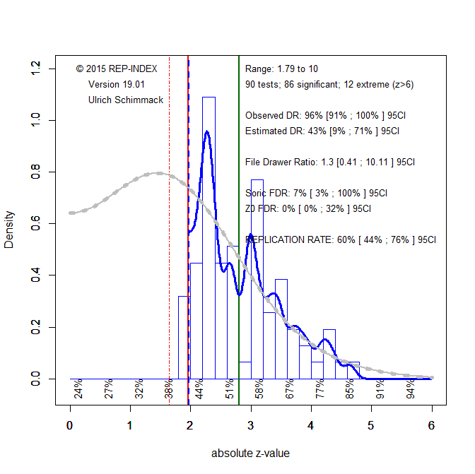
To demonstrate the implications of redefining the null-hypothesis, I use the results of the replicability project (Open Science Collaboration, 2015). The first z-curve shows the traditional analysis for the nil-hypothesis and alpha = .05, which has z = 1.96 as the criterion value for statistical significance (red vertical line).
Figure 1 shows that 86 out of 90 studies reported a test-statistic that exceeded the criterion value of 1.96 for H0:d = 0, alpha = .05 (two-tailed). The other four studies met the criterion for marginal significance (alpha = .10, two-tailed or .05 one-tailed). The figure also shows that the distribution of observed z-scores is not consistent with sampling error. The steep drop at z = 1.96 is inconsistent with random sampling error. A comparison of the observed discovery rate (86/90, 96%) and the expected discovery rate 43% shows evidence that the published results are selected from a larger set of studies/tests with non-significant results. Even the upper limit of the confidence interval around this estimate (71%) is well below the observed discovery rate, showing evidence of publication bias. Z-curve estimates that only 60% of the published results would reproduce a significant result in an actual replication attempt. The actual success rate for these studies was 39%.
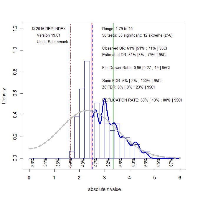
Results look different when the null-hypothesis is changed to correspond to a range of effect sizes around zero that correspond to a criterion value of z = 2.5. Along with shifting the significance criterion, z-curve is also only fitted to studies that produced z-scores greater than 2.5. As questionable research practices have a particularly strong effect on the distribution of just significant results, the new estimates are less influenced by these practices.
Figure 2 shows the results. Most important, the observed discovery rate dropped from 96% to 61%, indicating that many of the original results provided just enough evidence to reject the nil-hypothesis, but not enough evidence to rule out even small effect sizes. The observed discovery rate is also more in line with the expected discovery rate. Thus, some of the missing non-significant results may have been published as just significant results. This is also implied by the greater frequency of results with z-scores between 2 and 2.5 than the model predicts (grey curve). However, the expected replication rate of 63% is still much higher than the actual replication rate with a criterion value of 2.5 (33%). Thus, other factors may contribute to the low success rate in the actual replication studies of the replicability project.
Conclusion
In conclusion, statisticians have been arguing about p-values, significance levels, and Bayes-Factors. Proponents of Bayes-Factors have argued that their approach is supreme because Bayes-Factors can provide evidence for the null-hypothesis. I argue that this is wrong because it is theoretically impossible to demonstrate that a population effect size is exactly zero or any other specific value. A better solution is to specify the null-hypothesis as a range of values that are too small to be meaningful. This makes it theoretically possible to demonstrate that a population effect size is above or below the boundary value. This approach can also be applied retrospectively to published studies. I illustrate this by defining the null-hypothesis as the region of effect sizes that is defined by the effect size that corresponds to a z-score of 2.5. While a z-score of 2.5 corresponds to p = .01 (two-tailed) for the nil-hypothesis, I use this criterion value to maintain an error rate of 5% and to change the null-hypothesis to a range of values around zero that becomes smaller as sample sizes increase.
As p-hacking is often used to just reject the nil-hypothesis, changing the null-hypothesis to a range of values around zero makes many ‘significant’ results non-significant. That is, the evidence is too weak to exclude even trivial effect sizes. This does not mean that the hypothesis is wrong or that original authors did p-hack their data. However, it does mean that they can no longer point to their original results as empirical evidence. Rather they have to conduct new studies to demonstrate with larger samples that they can reject the new null-hypothesis that the predicted effect meets some minimal standard of practical or theoretical significance. With a clear criterion value for significance, authors also risk to obtain evidence that positively contradicts their predictions. Thus, the biggest improvement that arises form rethinking null-hypothesis testing is that authors have to specify effect sizes a priori and that that studies can provide evidence for and against a zero. Thus, changing the nil-hypothesis to a null-hypothesis with a non-null value makes it possible to provide evidence for or against a theory. In contrast, computing Bayes-Factors in favor of the nil-hypothesis fails to achieve this goal because the nil-hypothesis is always wrong, the real question is only how wrong.
1. We need to distinguish regions of effect sizes and precise values. The value 0 is a precise value. All positive values or all negative values are regions of values.
2. The most common use of null-hypothesis testing is to test whether the point-null or nil-hypothesis (Cohen, 1994) is consistent with the data.
3. Tukey explains that this hypothesis is likely to be false all the time. “All we know about the world teaches us that the effect of A and B are always different”. Many critics of NHST have suggested that this makes it useless to test the nil-hypothesis because we already know that it is false (the prior probability of H0 being true is 0, no data can change this).
4. NHST becomes useful when we think about the null-hypothesis (no difference) as the boundary value that distinguishes two regions. We are really testing the direction of the mean difference (or the sign of of a correlation coefficient). Once we can reject the nil-hypothesis (p < alpha) in a two-sided test, we are allowed to interpret the direction of the mean difference in a sample as the mean difference in the population (i.e., if we had studied all people from which the sample was drawn).
5. Some psychologists have criticized NHST because it can never provide evidence for the nil-hypothesis (Rouder, Wagenmakers). This criticism is based on a misunderstanding of NHST. Tukey explains we should never accept the nil-hypothesis because we can never provide empirical support FOR a precise effect size.
6. Once we have evidence that the nil-hypothesis is false and the effect is either positive or negative, we may ask follow-up questions about the size of an effect.
7. A good way to answer these questions is to conduct NHST with confidence intervals. If the confidence interval includes 0, we cannot draw inferences about the direction of the effect. However, if the confidence interval does not include 0, we can make inferences about the direction of an effect and the boundaries of the intervals provide information about plausible values for the smallest and the largest possible effect size.
8. In conclusion, we can think about two-sided tests as an efficient way of conducting two one-sided tests without inflating the type-I error probability. Rejecting the hypothesis that there is no effect is not interesting. Determining the direction of an effect is and NHST is a useful tool to do so.
9. I probably made things worse by paraphrasing Tukey. Therefore I also posted the relevant section of his article below.
Most psychologists are trained in Fisherian statistics, which has become known as Null-Hypothesis Significance Testing (NHST). NHST compares an observed effect size against a hypothetical effect size. The hypothetical effect size is typically zero; that is, the hypothesis is that there is no effect. The deviation of the observed effect size from zero relative to the amount of sampling error provides a test statistic (test statistic = effect size / sampling error). The test statistic can then be compared to a criterion value. The criterion value is typically chosen so that only 5% of test statistics would exceed the criterion value by chance alone. If the test statistic exceeds this value, the null-hypothesis is rejected in favor of the inference that an effect greater than zero was present.
One major problem of NHST is that non-significant results are not considered. To address this limitation, Neyman and Pearson extended Fisherian statistic and introduced the concepts of type-I (alpha) and type-II (beta) errors. A type-I error occurs when researchers falsely reject a true null-hypothesis; that is, they infer from a significant result that an effect was present, when there is actually no effect. The type-I error rate is fixed by the criterion for significance, which is typically p < .05. This means, that a set of studies cannot produce more than 5% false-positive results. The maximum of 5% false positive results would only be observed if all studies have no effect. In this case, we would expect 5% significant results and 95% non-significant results.
The important contribution by Neyman and Pearson was to consider the complementary type-II error. A type-II error occurs when an effect is present, but a study produces a non-significant result. In this case, researchers fail to detect a true effect. The type-II error rate depends on the size of the effect and the amount of sampling error. If effect sizes are small and sampling error is large, test statistics will often be too small to exceed the criterion value.
Neyman-Pearson statistics was popularized in psychology by Jacob Cohen. In 1962, Cohen examined effect sizes and sample sizes (as a proxy for sampling error) in the Journal of Abnormal and Social Psychology and concluded that there is a high risk of type-II errors because sample sizes are too small to detect even moderate effect sizes and inadequate to detect small effect sizes. Over the next decades, methodologists have repeatedly pointed out that psychologists often conduct studies with a high risk to fail; that is, to provide empirical evidence for real effects (Sedlemeier & Gigerenzer, 1989).
The concern about type-II errors has been largely ignored by empirical psychologists. One possible reason is that journals had no problem filling volumes with significant results, while rejecting 80% of submissions that also presented significant results. Apparently, type-II errors were much less common than methodologists feared.
However, in 2011 it became apparent that the high success rate in journals was illusory. Published results were not representative of studies that were conducted. Instead, researchers used questionable research practices or simply did not report studies with non-significant results. In other words, the type-II error rate was as high as methodologists suspected, but selection of significant results created the impression that nearly all studies were successful in producing significant results. The influential “False Positive Psychology” article suggested that it is very easy to produce significant results without an actual effect. This led to the fear that many published results in psychology may be false positive results.
Doubt about the replicability and credibility of published results has led to numerous recommendations for the improvement of psychological science. One of the most obvious recommendations is to ensure that published results are representative of the studies that are actually being conducted. Given the high type-II error rates, this would mean that journals would be filled with many non-significant and inconclusive results. This is not a very attractive solution because it is not clear what the scientific community can learn from an inconclusive result. A better solution would be to increase the statistical power of studies. Statistical power is simply the inverse of a type-II error (power = 1 – beta). As power increases, studies with a true effect have a higher chance of producing a true positive result (e.g., a drug is an effective treatment for a disease). Numerous articles have suggested that researchers should increase power to increase replicability and credibility of published results (e.g., Schimmack, 2012).
In a recent article, a team of 72 authors proposed another solution. They recommended that psychologists should reduce the probability of a type-I error from 5% (1 out of 20 studies) to 0.5% (1 out of 200 studies). This recommendation is based on the belief that the replication crisis in psychology reflects a large number of type-I errors. By reducing the alpha criterion, the rate of type-I errors will be reduced from a maximum of 10 out of 200 studies to 1 out of 200 studies.
I believe that this recommendation is misguided because it ignores the consequences of a more stringent significance criterion on type-II errors. Keeping resources and sampling error constant, reducing the type-I error rate increases the type-II error rate. This is undesirable because the actual type-II error is already large.
For example, a between-subject comparison of two means with a standardized effect size of d = .4 and a sample size of N = 100 (n = 50 per cell) has a 50% risk of a type-II error. The risk of a type-II error rises to 80%, if alpha is reduced to .005. It makes no sense to conduct a study with an 80% chance of failure (Tversky & Kahneman, 1971). Thus, the call for a lower alpha implies that researchers will have to invest more resources to discover true positive results. Many researchers may simply lack the resources to meet this stringent significance criterion.
My suggestion is exactly opposite to the recommendation of a more stringent criterion. The main problem for selection bias in journals is that even the existing criterion of p < .05 is too stringent and leads to a high percentage of type-II errors that cannot be published. This has produced the replication crisis with large file-drawers of studies with p-values greater than .05, the use of questionable research practices, and publications of inflated effect sizes that cannot be replicated.
To avoid this problem, researchers should use a significance criterion that balances the risk of a type-I and type-II error. For example, in a between-subject design with an expected effect size of d = .4 and N = 100, researchers should use p < .20 for significance, which reduces the risk of a type -II error to 20%. In this case, type-I and type-II error are balanced. If the study produces a p-value of, say, .15, researchers can publish the result with the conclusion that the study provided evidence for the effect. At the same time, readers are warned that they should not interpret this result as strong evidence for the effect because there is a 20% probability of a type-I error.
Given this positive result, researchers can then follow up their initial study with a larger replication study that allows for a stricter type-I error control, while holding power constant. With d = 4, they now need N = 200 participants to have 80% power and alpha = .05. Even if the second study does not produce a significant result (the probability that two studies with 80% power are significant is only 64%, Schimmack, 2012), researchers can combine the results of both studies and with N = 300, the combined studies have 80% power with alpha = .01.
The advantage of starting with smaller studies with a higher alpha criterion is that researchers are able to test risky hypothesis with a smaller amount of resources. In the example, the first study used “only” 100 participants. In contrast, the proposal to require p < .005 as evidence for an original, risky study implies that researchers need to invest a lot of resources in a risky study that may provide inconclusive results if it fails to produce a significant result. A power analysis shows that a sample size of N = 338 participants is needed to have 80% power for an effect size of d = .4 and p < .005 as criterion for significance.
Rather than investing 300 participants into a risky study that may produce a non-significant and uninteresting result (eating green jelly beans does not cure cancer), researchers may be better able and willing to start with 100 participants and to follow up an encouraging result with a larger follow-up study. The evidential value that arises from one study with 300 participants or two studies with 100 and 200 participants is the same, but requiring p < .005 from the start discourages risky studies and puts even more pressure on researchers to produce significant results if all of their resources are used for a single study. In contrast, lowering alpha reduces the need for questionable research practices and reduces the risk of type-II errors.
In conclusion, it is time to learn Neyman-Pearson statistic and to remember Cohen’s important contribution that many studies in psychology are underpowered. Low power produces inconclusive results that are not worthwhile publishing. A study with low power is like a high-jumper that puts the bar too high and fails every time. We learned nothing about the jumpers’ ability. Scientists may learn from high-jump contests where jumpers start with lower and realistic heights and then raise the bar when they succeeded. In the same manner, researchers should conduct pilot studies or risky exploratory studies with small samples and a high type-I error probability and lower the alpha criterion gradually if the results are encouraging, while maintaining a reasonably low type-II error.
Evidently, a significant result with alpha = .20 does not provide conclusive evidence for an effect. However, the arbitrary p < .005 criterion also fails short of demonstrating conclusively that an effect exists. Journals publish thousands of results a year and some of these results may be false positives, even if the error rate is set at 1 out of 200. Thus, p < .005 is neither defensible as a criterion for a first exploratory study, nor conclusive evidence for an effect. A better criterion for conclusive evidence is that an effect can be replicated across different laboratories and a type-I error probability of less than 1 out of a billion (6 sigma). This is by no means an unrealistic target. To achieve this criterion with an effect size of d = .4, a sample size of N = 1,000 is needed. The combined evidence of 5 labs with N = 200 per lab would be sufficient to produce conclusive evidence for an effect, but only if there is no selection bias. Thus, the best way to increase the credibility of psychological science is to conduct studies with high power and to minimize selection bias.
This is what I believe Cohen would have said, but even if I am wrong about this, I think it follows from his futile efforts to teach psychologists about type-II errors and statistical power.
In 2005, John P. A. Ioannidis wrote an influential article with the title “Why Most Published Research Findings are False.” The article starts with the observation that “there is increasing concern that most current published research findings are false” (e124). Later on, however, the concern becomes a fact. “It can be proven that most claimed research findings are false” (e124). It is not surprising that an article that claims to have proof for such a stunning claim has received a lot of attention (2,199 citations and 399 citations in 2016 alone in Web of Science).
Most citing articles focus on the possibility that many or even more than half of all published results could be false. Few articles cite Ioannidis to make the factual statement that most published results are false, and there appears to be no critical examination of Ioannidis’s simulations that he used to support his claim.
This blog post shows that these simulations make questionable assumptions and shows with empirical data that Ioannidis’s simulations are inconsistent with actual data.
Critical Examination of Ioannidis’s Simulations
First, it is important to define what a false finding is. In many sciences, a finding is published when a statistical test produced a significant result (p < .05). For example, a drug trial may show a significant difference between a drug and a placebo control condition with a p-value of .02. This finding is then interpreted as evidence for the effectiveness of the drug.
How could this published finding be false? The logic of significance testing makes this clear. The only inference that is being made is that the population effect size (i.e., the effect size that could be obtained if the same experiment were repeated with an infinite number of participants) is different from zero and in the same direction as the one observed in the study. Thus, the claim that most significant results are false implies that in more than 50% of all published significant results the null-hypothesis was true. That is, a false positive result was reported.
Ioannidis then introduces the positive predictive value (PPV). The positive predictive value is the proportion of positive results (p < .05) that are true positives.
The proportion of true positive results (TP) depends on the percentage of true hypothesis (PTH) and the probability of producing a significant result when a hypothesis is true. This probability is known as statistical power. Statistical power is typically defined as 1 minus the type-II error (beta).
(2) TP = PTH * Power = PTH * (1 – beta)
The probability of a false positive result depends on the proportion of false hypotheses (PFH) and the criterion for significance (alpha).
(3) FP = PFH * alpha
This means that the actual proportion of true significant results is a function of the ratio of true and false hypotheses (PTH:PFH), power, and alpha.
Ioannidis translates his claim that most published findings are false into a PPV below 50%. This would mean that the null-hypothesis is true in more than 50% of published results that falsely rejected it.
Equation (5) can be simplied to the inequality equation
(6) alpha > PTH/PFH * power
We can rearrange formula (6) and substitute PFH with (1-PHT) to determine the maximum proportion of true hypotheses to produce over 50% false positive results.
Even if researchers would conduct studies with only 20% power to discover true positive results, we would only obtain more than 50% false positive results if only 20% of hypothesis were true. This makes it rather implausible that most published results could be false.
To justify his bold claim, Ioannidis introduces the notion of bias. Bias can be introduced due to various questionable research practices that help researchers to report significant results. The main effect of these practices is that the probability of a false positive result to become significant increases.
Simmons et al. (2011) showed that massive use several questionable research practices (p-hacking) can increase the risk of a false positive result from the nominal 5% to 60%. If we assume that bias is rampant and substitute the nominal alpha of 5% with an assumed alpha of 50%, fewer false hypotheses are needed to produce more false than true positives (Table 2).
If we assume that bias inflates the risk of type-I errors from 5% to 60%, it is no longer implausible that most research findings are false. In fact, more than 50% of published results would be false if researchers tested hypothesis with 50% power and 50% of tested hypothesis are false.
However, the calculations in Table 2 ignore the fact that questionable research practices that inflate false positives also decrease the rate of false negatives. For example, a researcher who continues testing until a significant result is obtained, increases the chances of obtaining a significant result no matter whether the hypothesis is true or false.
Ioannidis recognizes this, but he assumes that bias has the same effect for true hypothesis and false hypothesis. This assumption is questionable because it is easier to produce a significant result if an effect exists than if no effect exists. Ioannidis’s assumption implies that bias increases the proportion of false positive results a lot more than the proportion of true positive results.
For example, if power is 50%, only 50% of true hypothesis produce a significant result. However, with a bias factor of .4, another 40% of the false negative results will become significant, adding another .4*.5 = 20% true positive results to the number of true positive results. This gives a total of 70% positive results, which is a 40% increase over the number of positive results that would have been obtained without bias. However, this increase in true positive results pales in comparison to the effect that 40% bias has on the rate of false positives. As there are 95% true negatives, 40% bias produces another .95*.40 = 38% of false positive results. So instead of 5% false positive results, bias increases the percentage of false positive results from 5% to 43%, an increase by 760%. Thus, the effect of bias on the PPV is not equal. A 40% increase of false positives has a much stronger impact on the PPV than a 40% increase of true positives. Ioannidis provides no rational for this bias model.
A bigger concern is that Ioannidis makes sweeping claims about the proportion of false published findings based on untested assumptions about the proportion of null-effects, statistical power, and the amount of bias due to questionable research practices.
For example, he suggests that 4 out of 5 discoveries in adequately powered (80% power) exploratory epidemiological studies are false positives (PPV = .20). To arrive at this estimate, he assumes that only 1 out of 11 hypotheses is true and that for every 1000 studies, bias adds only 1000* .30*.10*.20 = 6 true positives results compared to 1000* .30*.90*.95 = 265 false positive results (i.e., 44:1 ratio). The assumed bias turns a PPV of 62% without bias into a PPV of 20% with bias. These untested assumptions are used to support the claim that “simulations show that for most study designs and settings, it is more likely for a research claim to be false than true.” (e124).
Many of these assumptions can be challenged. For example, statisticians have pointed out that the null-hypothesis is unlikely to be true in most studies (Cohen, 1994). This does not mean that all published results are true, but Ioannidis’ claims rest on the opposite assumption that most hypothesis are a priori false. This makes little sense when the a priori hypothesis is specified as a null-effect and even a small effect size is sufficient for a hypothesis to be correct.
Ioannidis also ignores attempts to estimate the typical power of studies (Cohen, 1962). At least in psychology, the typical power is estimated to be around 50%. As shown in Table 2, even massive bias would still produce more true than false positive results, if the null-hypothesis is false in no more than 50% of all statistical tests.
In conclusion, Ioannidis’s claim that most published results are false depends heavily on untested assumptions and cannot be considered a factual assessment of the actual number of false results in published journals.
Testing Ioannidis’s Simulations
10 years after the publication of “Why Most Published Research Findings Are False,” it is possible to put Ioannidis’s simulations to an empirical test. Powergraphs (Schimmack, 2015) can be used to estimate the average replicability of published test results. For this purpose, each test statistic is converted into a z-value. A powergraph is foremost a histogram of z-values. The distribution of z-values provides information about the average statistical power of published results because studies with higher power produce higher z-values.
Figure 1 illustrates the distribution of z-values that is expected for Ioanndis’s model for “adequately powered exploratory epidemiological study” (Simulation 6 in Figure 4). Ioannidis assumes that for every true positive, there are 10 false positives (R = 1:10). He also assumed that studies have 80% power to detect a true positive. In addition, he assumed 30% bias.
A 30% bias implies that for every 100 false hypotheses, there would be 33 (100*[.30*.95+.05]) rather than 5 false positive results (.95*.30+.05)/.95). The effect on false negatives is much smaller (100*[.30*.20 + .80]). Bias was modeled by increasing the number of attempts to produce a significant result so that proportion of true and false hypothesis matched the predicted proportions. Given an assumed 1:10 ratio of true to false hypothesis, the ratio is 335 false hypotheses to 86 true hypotheses. The simulation assumed that researchers tested 100,000 false hypotheses and observed 35000 false positive results and that they tested 10,000 true hypotheses and observed 8,600 true positive results. Bias was simulated by increasing the number of tests to produce the predicted ratio of true and false positive results.
Figure 1 only shows significant results because only significant results would be reported as positive results. Figure 1 shows that a high proportion of z-values are in the range between 1.95 (p = .05) and 3 (p = .001). Powergraphs use z-curve (Schimmack & Brunner, 2016) to estimate the probability that an exact replication study would replicate a significant result. In this simulation, this probability is a mixture of false positives and studies with 80% power. The true average probability is 20%. The z-curve estimate is 21%. Z-curve can also estimate the replicability for other sets of studies. The figure on the right shows replicability for studies that produced an observed z-score greater than 3 (p < .001). The estimate shows an average replicability of 59%. Thus, researchers can increase the chance of replicating published findings by adjusting the criterion value and ignoring significant results with p-values greater than p = .001, even if they were reported as significant with p < .05.
Figure 2 shows the distribution of z-values for Ioannidis’s example of a research program that produces more true than false positives, PPV = .85 (Simulation 1 in Table 4).
Visual inspection of Figure 1 and Figure 2 is sufficient to show that a robust research program produces a dramatically different distribution of z-values. The distribution of z-values in Figure 2 and a replicability estimate of 67% are impossible if most of the published significant results were false. The maximum value that could be obtained is obtained with a PPV of 50% and 100% power for the true positive results, which yields a replicability estimate of .05*.50 + 1*.50 = 55%. As power is much lower than 100%, the real maximum value is below 50%.
The powergraph on the right shows the replicability estimate for tests that produced a z-value greater than 3 (p < .001). As only a small proportion of false positives are included in this set, z-curve correctly estimates the average power of these studies as 80%. These examples demonstrate that it is possible to test Ioannidis’s claim that most published (significant) results are false empirically. The distribution of test results provides relevant information about the proportion of false positives and power. If actual data are more similar to the distribution in Figure 1, it is possible that most published results are false positives, although it is impossible to distinguish false positives from false negatives with extremely low power. In contrast, if data look more like those in Figure 2, the evidence would contradict Ioannidis’s bold and unsupported claim that most published results are false.
The maximum replicabiltiy that could be obtained with 50% false-positives would require that the true positive studies have 100% power. In this case, replicability would be .50*.05 + .50*1 = 52.5%. However, 100% power is unrealistic. Figure 3 shows the distribution for a scenario with 90% power and 100% bias and an equal percentage of true and false hypotheses. The true replicabilty for this scenario is .05*.50 + .90 * .50 = 47.5%. z-curve slightly overestimates replicabilty and produced an estimate of 51%. Even 90% power is unlikely in a real set of data. Thus, replicability estimates above 50% are inconsistent with Ioannidis’s hypothesis that most published positive results are false. Moreover, the distribution of z-values greater than 3 is also informative. If positive results are a mixture of many false positive results and true positive results with high power, the replicabilty estimate for z-values greater than 3 should be high. In contrast, if this estimate is not much higher than the estimate for all z-values, it suggest that there is a high proportion of studies that produced true positive results with low power.
Empirical Evidence
I have produced powergraphs and replicability estimates for over 100 psychology journals (2015 Replicabilty Rankings). Not a single journal produced a replicability estimate below 50%. Below are a few selected examples.
The Journal of Experimental Psychology: Learning, Memory and Cognition publishes results from cognitive psychology. In 2015, a replication project (OSC, 2015) demonstrated that 50% of significant results produced a significant result in a replication study. It is unlikely that all non-significant results were false positives. Thus, the results show that Ioannidis’s claim that most published results are false does not apply to results published in this journal.
The powergraphs further support this conclusion. The graphs look a lot more like Figure 2 than Figure 1 and the replicability estimate is even higher than the one expected from Ioannidis’s simulation with a PPV of 85%.
Another journal that was subjected to replication attempts was Psychological Science. The success rate for Psychological Science was below 50%. However, it is important to keep in mind that a non-significant result in a replication study does not prove that the original result was a false positive. Thus, the PPV could still be greater than 50%.
The powergraph for Psychological Science shows more z-values in the range between 2 and 3 (p > .001). Nevertheless, the replicability estimate is comparable to the one in Figure 2 which simulated a high PPV of 85%. Closer inspection of the results published in this journal would be required to determine whether a PPV below .50 is plausible.
The third journal that was subjected to a replication attempt was the Journal of Personality and Social Psychology. The journal has three sections, but I focus on the Attitude and Social Cognition section because many replication studies were from this section. The success rate of replication studies was only 25%. However, there is controversy about the reason for this high number of failed replications and once more it is not clear what percentage of failed replications were due to false positive results in the original studies.
One problem with the journal rankings is that they are based on automated extraction of all test results. Ioannidis might argue that his claim focused only on test results that tested an original, novel, or an important finding, whereas articles also often report significance tests for other effects. For example, an intervention study may show a strong decrease in depression, when only the interaction with treatment is theoretically relevant.
I am currently working on powergraphs that are limited to theoretically important statistical tests. These results may show lower replicability estimates. Thus, it remains to be seen how consistent Ioannidis’s predictions are for tests of novel and original hypotheses. Powergraphs provide a valuable tool to address this important question.
Moreover, powergraphs can be used to examine whether science is improving. So far, powergraphs of psychology journals have shown no systematic improvement in response to concerns about high false positive rates in published journals. The powergraphs for 2016 will be published soon. Stay tuned.
The editor of Psychological Science published an Editorial with the title “Business Not as Usual.” (see also Observer interview and new Submission Guidelines) The new submission guidelines recommend the following statistical approach.
Effective January 2014, Psychological Science recommends the use of the “new statistics”—effect sizes, confidence intervals, and meta-analysis—to avoid problems associated with null-hypothesis significance testing (NHST). Authors are encouraged to consult this Psychological Science tutorial by Geoff Cumming, which shows why estimation and meta-analysis are more informative than NHST and how they foster development of a cumulative, quantitative discipline. Cumming has also prepared a video workshop on the new statistics that can be found here.
The editorial is a response to the current crisis in psychology that many findings cannot be replicated and the discovery that numerous articles in Psychological Science show clear evidence of reporting biases that lead to inflated false-positive rates and effect sizes (Francis, 2013).
The editorial is titled “Business not as usual.” So what is the radical response that will ensure increased replicability of results published in Psychological Science? One solution is to increase transparency and openness to discourage the use of deceptive research practices (e.g., not publishing undesirable results or selective reporting of dependent variables that showed desirable results). The other solution is to abandon null-hypothesis significance testing.
Problem of the Old Statistics: Researchers had to demonstrate that their empirical results could have occurred only with a 5% probability if there is no effect in the population.
Null-hypothesis testing has been the main method to relate theories to empirical data. An article typically first states a theory and then derives a theoretical prediction from the theory. The theoretical prediction is then used to design a study that can be used to test the theoretical prediction. The prediction is tested by computing the ratio of the effect size and sampling error (signal-to-noise) ratio. The next step is to determine the probability of obtaining the observed signal-to-noise ratio or an even more extreme one under the assumption that the true effect size is zero. If this probability is smaller than a criterion value, typically p < .05, the results are interpreted as evidence that the theoretical prediction is true. If the probability does not meet the criterion, the data are considered inconclusive.
However, non-significant results are irrelevant because Psychological Science is only interested in publishing research that supports innovative novel findings. Nobody wants to know that drinking fennel tea does not cure cancer, but everybody wants to know about a treatment that actually cures cancer. So, the main objective of statistical analyses was to provide empirical evidence for a predicted effect by demonstrating that an obtained result would occur only with a 5% probability if the hypothesis were false.
Solution to the problem of Significance Testing: Drop the Significance Criterion. Just report your sample mean and the 95% confidence interval around it.
Eich claims that “researchers have recognized,…, essential problems with NHST in general, and with dichotomous thinking (“significant” vs. “non-significant” ) thinking it engenders in particular. It is true that statisticians have been arguing about the best way to test theoretical predictions with empirical data. In fact, they are still arguing. Thus, it is interesting to examine how Psychological Science found a solution to the elusive problem of statistical inference. The answer is to avoid statistical inferences altogether and to avoid dichotomous thinking. Does fennel tea cure cancer? Maybe, 95%CI d = -.4 to d = +4. No need to test for statistical significance. No need to worry about inadequate sample sizes. Just do a study and report your sample means with a confidence interval. It is that easy to fix the problems of psychological science.
The problem is that every study produces a sample mean and a confidence interval. So, how do the editors of Psychological Science pick the 5% of submitted manuscripts that will be accepted for publication? Eich lists three criteria.
What will the reader of this article learn about psychology that he or she did not know (or could not have known) before?
The effect of manipulation X on dependent variable Y is d = .2, 95%CI = -.2 to .6. We can conclude from this result that it is unlikely that the manipulation leads to a moderate decrease or a strong increase in the dependent variable Y.
Why is that knowledge important for the field?
The finding that the experimental manipulation of Y in the laboratory is somewhat more likely to produce an increase than a decrease, but could also have no effect at all has important implications for public policy.
How are the claims made in the article justified by the methods used?
The claims made in this article are supported by the use of Cumming’s New Statistics. Based on a precision analysis, the sample size was N = 100 (n = 50 per condition) to achieve a precision of .4 standard deviations. The study was preregistered and the data are publicly available with the code to analyze the data (SPPS t-test groups x (1,2) / var y.).
If this sounds wrong to you and you are a member of APS, you may want to write to Erich Eich and ask for some better guidelines that can be used to evaluate whether a sample mean or two or three or four sample means should be published in your top journal.
Cookie Consent
We use cookies to improve your experience on our site. By using our site, you consent to cookies.