Category Archives: Observed Discovery Rate

The Prevalence of Questionable Research Practices in Social Psychology

Introduction

A naive model of science assumes that scientists are objective. That is, they derive hypotheses from theories, collect data to test these theories, and then report the results. In reality, scientists are passionate about theories and often want to confirm that their own theories are right. This leads to conformation bias and the use of questionable research practices (QRPs, John et al., 2012; Schimmack, 2015). QRPs are defined as practices that increase the chances of the desired outcome (typically a statistically significant result) while at the same time inflating the risk of a false positive discovery. A simple QRP is to conduct multiple studies and to report only the results that support the theory.

The use of QRPs explains the astonishingly high rate of statistically significant results in psychology journals that is over 90% (Sterling, 1959; Sterling et al., 1995). While it is clear that this rate of significant results is too high, it is unclear how much it is inflated by QRPs. Given the lack of quantitative information about the extent of QRPs, motivated biases also produce divergent opinions about the use of QRPs by social psychologists. John et al. (2012) conducted a survey and concluded that QRPs are widespread. Fiedler and Schwarz (2016) criticized the methodology and their own survey of German psychologists suggested that QRPs are not used frequently. Neither of these studies is ideal because they relied on self-report data. Scientists who heavily use QRPs may simply not participate in surveys of QRPs or underreport the use of QRPs. It has also been suggested that many QRPs happen automatically and are not accessible to self-reports. Thus, it is necessary to study the use of QRPs with objective methods that reflect the actual behavior of scientists. One approach is to compare dissertations with published articles (Cairo et al., 2020). This method provided clear evidence for the use of QRPs, even though a published document could reveal their use. It is possible that this approach underestimates the use of QRPs because even the dissertation results could be influenced by QRPs and the supervision of dissertations by outsiders may reduce the use of QRPs.

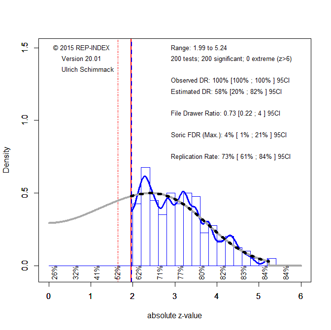
With my colleagues, I developed a statistical method that can detect and quantify the use of QRPs (Bartos & Schimmack, 2020; Brunner & Schimmack, 2020). Z-curve uses the distribution of statistically significant p-values to estimate the mean power of studies before selection for significance. This estimate predicts how many non-significant results were obtained in the serach for the significant ones. This makes it possible to compute the estimated discovery rate (EDR). The EDR can then be compared to the observed discovery rate, which is simply the percentage of published results that are statistically significant. The bigger the difference between the ODR and the EDR is, the more questionable research practices were used (see Schimmack, 2021, for a more detailed introduction).

I merely focus on social psychology because (a) I am a social/personality psychologists, who is interested in the credibility of results in my field, and (b) because social psychology has a large number of replication failures (Schimmack, 2020). Similar analyses are planned for other areas of psychology and other disciplines. I also focus on social psychology more than personality psychology because personality psychology is often more exploratory than confirmatory.

Method

I illustrate the use of z-curve to quantify the use of QRPs with the most extreme examples in the credibility rankings of social/personality psychologists (Schimmack, 2021). Figure 1 shows the z-value plot (ZVP) of David Matsumoto. To generate this plot, the tests statistics from t-tests and F-tests were transformed into exact p-values and then transformed into the corresponding values on the standard normal distribution. As two-sided p-values are used, all z-scores are positive. However, because the curve is centered over the z-score that corresponds to the median power before selection for significance (and not zero, when the null-hypothesis is true), the distribution can look relatively normal. The variance of the distribution will be greater than 1 when studies vary in statistical power.

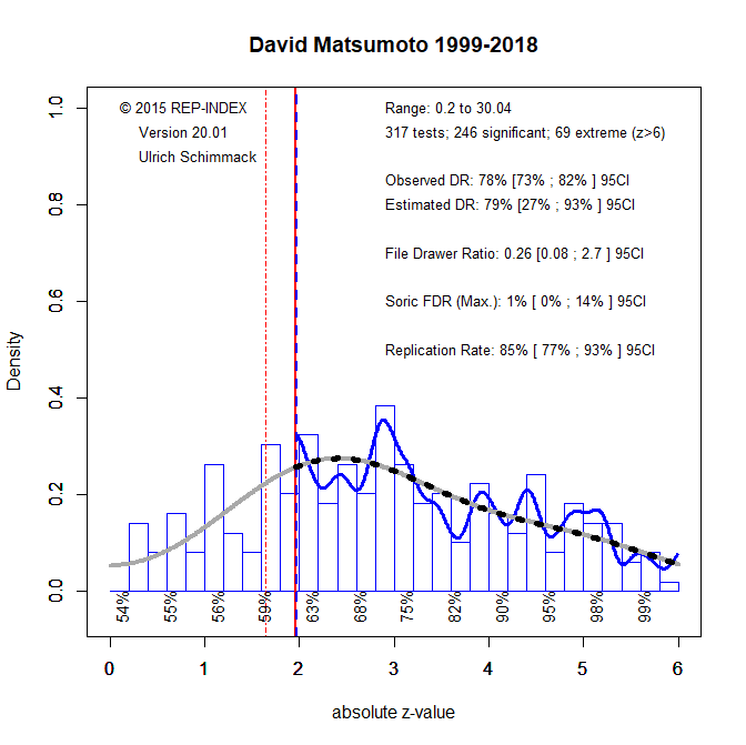
The grey curve in Figure 1 shows the predicted distribution based on the observed distribution of z-scores that are significant (z > 1.96). In this case, the observed number of non-significant results is similar to the predicted number of significant results. As a result, the ODR of 78% closely matches the EDR of 79%.

Figure 2 shows the results for Shelly Chaiken. The first notable observation is that the ODR of 75% is very similar to Matsumoto’s EDR of 78%. Thus, if we simply count the number of significant and non-significant p-values, there is no difference between these two researchers. However, the z-value plot (ZVP) shows a dramatically different picture. The peak density is 0.3 for Matsoumoto and 1.0 for Chaiken. As the maximum density of the standard normal distribution is .4, it is clear that the results in Chaiken’s articles are not from an actual sampling distribution. In other words, QRPs must have been used to produce too many just significant results with p-values just below .05.

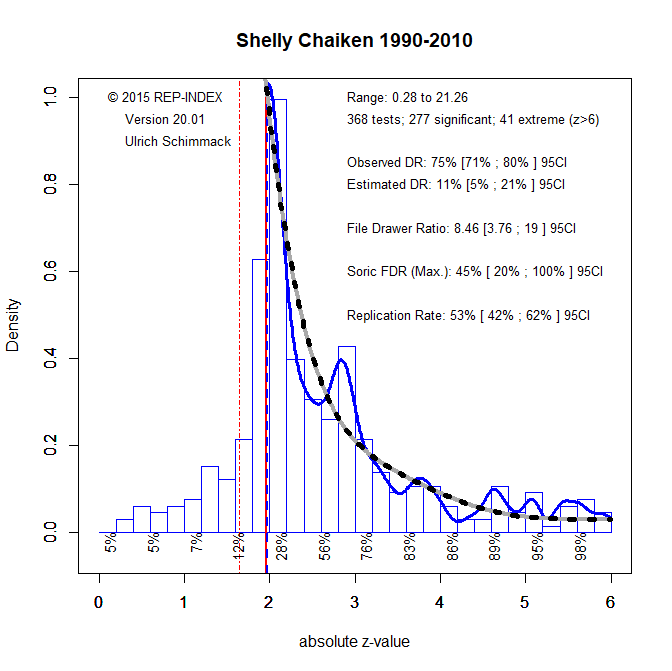
The comparison of the ODR and EDR shows a large discrepancy of 64 percentage points too many significant results (ODR = 75% minus EDR = 11%). This is clearly not a chance finding because the ODR falls well outside the 95% confidence interval of the EDR, 5% to 21%.

To examine the use of QPSs in social psychology, I computed the EDR and ORDR for over 200 social/personality psychologists. Personality psychologists were excluded if they reported too few t-values and F-values. The actual values can be found and additional statistics can be found in the credibility rankings (Schimmack, 2021). Here I used these data to examine the use of QRPs in social psychology.

Average Use of QRPs

The average ODR is 73.48 with a 95% confidence interval ranging from 72.67 to 74.29. The average EDR is 35.28 with a 95% confidence interval ranging from 33.14 to 37.43. the inflation due to QRPs is 38.20 percentage points, 95%CI = 36.10 to 40.30. This difference is highly significant, t(221) = 35.89, p < too many zeros behind the decimal for R to give an exact value.

It is of course not surprising that QRPs have been used. More important is the effect size estimate. The results suggest that QRPs inflate the discovery rate by over 100%. This explains why unbiased replication studies in social psychology have only a 25% chance of being significant (Open Science Collaboration, 2015). In fact, we can use the EDR as a conservative predictor of replication outcomes (Bartos & Schimmack, 2020). While the EDR of 35% is a bit higher than the actual replication rate, this may be due to the inclusion of non-focal hypothesis tests in these analyses. Z-curve analyses of focal hypothesis tests typically produce lower EDRs. In contrast, Fiedler and Schwarz failed to comment on the low replicability of social psychology. If social psychologists would not have used QRPs, it remains a mystery why their results are so hard to replicate.

In sum, the present results confirm that, on average, social psychologists heavily used QRPs to produce significant results that support their predictions. However, these averages masks differences between researchers like Matsumoto and Chaiken. The next analyses explore these individual differences between researchers.

Cohort Effects

I had no predictions about the effect of cohort on the use of QRPs. I conducted a twitter poll that suggested a general intuition that the use of QRPs may not have changed over time, but there was a lot of uncertainty in these answers. Similar results were obtained in a Facebook poll in the Psychological Methods Discussion Group. Thus, the a priori hypothesis is a vague prior of no change.

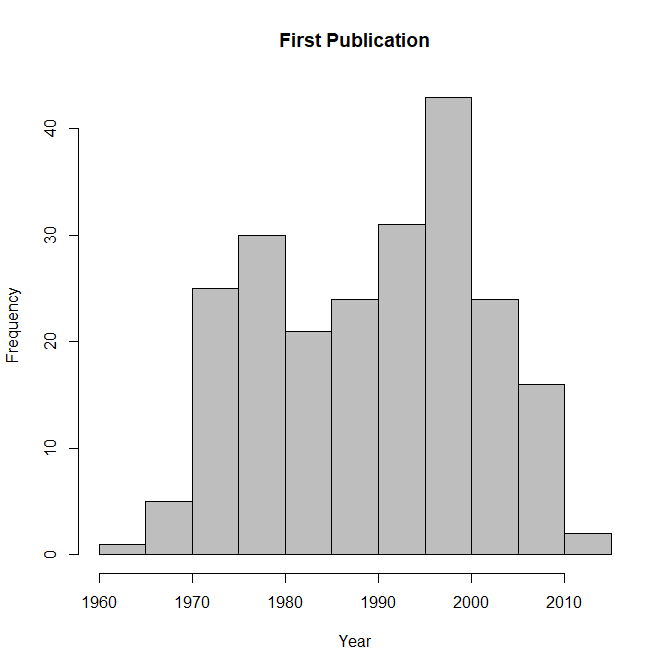
The dataset includes different generations of researchers. I used the first publication listed in WebofScience to date researchers. The earliest date was 1964 (Robert S. Wyer). The latest date was 2012 (Kurt Gray). The histogram shows that researchers from the 1970s to 2000s were well-represented in the dataset.

There was a significant negative correlation between the ODR and cohort, r(N = 222) = -.25, 95%CI = -.12 to -.37, t(220) = 3.83, p = .0002. This finding suggests that over time the proportion of non-significant results increased. For researchers with the first publication in the 1970s, the average ODR was 76%, whereas it was 72% for researchers with the first publication in the 2000s. This is a modest trend. There are various explanations for this trend.

One possibility is that power decreased as researchers started looking for weaker effects. In this case, the EDR should also show a decrease. However, the EDR showed no relationship with cohort, r(N = 222) = -.03, 95%CI = -.16 to .10, t(220) = 0.48, p = .63. Thus, less power does not seem to explain the decrease in the ODR. At the same time, the finding that EDR does not show a notable, abs(r) < .2, relationship with cohort suggests that power has remained constant over time. This is consistent with previous examinations of statistical power in social psychology (Sedlmeier & Gigerenzer, 1989).

Although the ODR decreased significantly and the EDR did not decrease significantly, bias (ODR – EDR) did not show a significant relationship with cohort, r(N = 222) = -.06, 95%CI = -19 to .07, t(220) = -0.94, p = .35, but the 95%CI allows for a slight decrease in bias that would be consistent with the significant decrease in the ODR.

In conclusion, there is a small, statistically significant decrease in the ODR, but the effect over the past 40 decades is too small to have practical significance. The EDR and bias are not even statistically significantly related to cohort. These results suggest that research practices and the use of questionable ones has not changed notably since the beginning of empirical social psychology (Cohen, 1961; Sterling, 1959).

Achievement Motivation

Another possibility is that in each generation, QRPs are used more by researches who are more achievement motivated (Janke et al., 2019). After all, the reward structure in science is based on number of publications and significant results are often needed to publish. In social psychology it is also necessary to present a package of significant results across multiple studies, which is nearly impossible without the use of QRPs (Schimmack, 2012). To examine this hypothesis, I correlated the EDR with researchers’ H-Index (as of 2/1/2021). The correlation was small, r(N = 222) = .10, 95%CI = -.03 to .23, and not significant, t(220) = 1.44, p = .15. This finding is only seemingly inconsistent with Janke et al.’s (2019) finding that self-reported QRPs were significantly correlated with self-reported ambition, r(217) = .20, p = .014. Both correlations are small and positive, suggesting that achievement motivated researchers may be slightly more likely to use QRPs. However, the evidence is by no means conclusive and the actual relationship is weak. Thus, there is no evidence to support that highly productive researchers with impressive H-indices achieved their success by using QRPs more than other researchers. Rather, they became successful in a field where QRPs are the norm. If the norms were different, they would have become successful following these other norms.

Impact

A common saying in science is that “extraordinary claims require extraordinary evidence.” Thus, we might expect stronger evidence for claims of time-reversed feelings (Bem, 2011) than for evidence that individuals from different cultures regulate their emotions differently (Matsumoto et al., 2008). However, psychologists have relied on statistical significance with alpha = .05 as a simple rule to claim discoveries. This is a problem because statistical significance is meaningless when results are selected for significance and replication failures with non-significant results remain unpublished (Sterling, 1959). Thus, psychologists have trusted an invalid criterion that does not distinguish between true and false discoveries. It is , however, possible that social psychologists used other information (e.g, gossip about replication failures at conferences) to focus on credible results and to ignore incredible ones. To examine this question, I correlated authors’ EDR with the number of citations in 2019. I used citation counts for 2019 because citation counts for 2020 are not yet final (the results will be updated with the 2020 counts). Using 2019 increases the chances of finding a significant relationship because replication failures over the past decade could have produced changes in citation rates.

The correlation between EDR and number of citations was statistically significant, r(N = 222) = .16, 95%CI = .03 to .28, t(220) = 2.39, p = .018. However, the lower limit of the 95% confidence interval is close to zero. Thus, it is possible that the real relationship is too small to matter. Moreover, the non-parametric correlation with Kendell’s tau was not significant, tau = .085, z = 1.88, p = .06. Thus, at present there is insufficient evidence to suggest that citation counts take the credibility of significant results into account. At present, p-values less than .05 are treated as equally credible no matter how they were produced.

Conclusion

There is general agreement that questionable research practices have been used to produce an unreal success rate of 90% or more in psychology journals (Sterling, 1959). However, there is less agreement about the amount of QRPs that are being used and the implications for the credibility of significant results in psychology journals (John et al., 2012; Fiedler & Schwarz, 2016). The problem is that self-reports may be biased because researchers are unable or unwilling to report the use of QRPs (Nisbett & Wilson, 1977). Thus, it is necessary to examine this question with alternative methods. The present study used a statistical method to compare the observed discovery rate with a statistically estimated discovery rate based on the distribution of significant p-values. The results showed that on average social psychologists have made extensive use of QRPs to inflate an expected discovery rate of around 35% to an observed discovery rate of 70%. Moreover, the estimated discovery rate of 35%is likely to be an inflated estimate of the discovery rate for focal hypothesis tests because the present analysis is based on focal and non-focal tests. This would explain why the actual success rate in replication studies is even lower thna the estimated discovery rate of 35% (Open Science Collaboration, 2015).

The main novel contribution of this study was to examine individual differences in the use of QRPs. While the ODR was fairly consistent across articles, the EDR varied considerably across researchers. However, this variation showed only very small relationships with a researchers’ cohort (first year of publication). This finding suggests that the use of QRPs varies more across research fields and other factors than over time. Additional analysis should explore predictors of the variation across researchers.

Another finding was that citations of authors’ work do not take credibility of p-values into account. Citations are influenced by popularity of topics and other factors and do not take the strength of evidence into account. One reason for this might be that social psychologists often publish multiple internal replications within a single article. This gives the illusion that results are robust and credible because it is very unlikely to replicate type-I errors. However, Bem’s (2011) article with 9 internal replications of time-reversed feelings showed that QRPs are also used to produce consistent results within a single article (Francis, 2012; Schimmack, 2012). Thus, number of significant results within an article or across articles is also an invalid criterion to evaluate the robustness of results.

In conclusion, social psychologists have conducted studies with low statistical power since the beginning of empirical social psychology. The main reason for this is the preference for between-subject designs that have low statistical power with small sample sizes of N = 40 participants and small to moderate effect sizes. Despite repeated warnings about the problems of selection for significance (Sterling, 1959) and the problems of small sample sizes (Cohen, 1961; Sedelmeier & Gigerenzer, 1989; Tversky & Kahneman, 1971), the practices have not changed since Festinger conducted his seminal study on dissonance with n = 20 per group. Over the past decades, social psychology journals have reported thousands of statistically significant results that are used in review articles, meta-analyses, textbooks, and popular books as evidence to support claims about human behavior. The problem is that it is unclear which of these significant results are true positives and which are false positives, especially if false positives are not just strictly nil-results, but also results with tiny effect sizes that have no practical significance. Without other reliable information, even social psychologists do not know which of their colleagues results are credible or not. Over the past decade, the inability to distinguish credible and incredible information has produced heated debates and a lack of confidence in published results. The present study shows that the general research practices of a researcher provide valuable information about credibility. For example, a p-value of .01 by a researcher with an EDR of 70 is more credible than a p-value of .01 by a researcher with an EDR of 15. Thus, rather than stereotyping social psychologists based on the low replication rate in the Open Science Collaboration project, social psychologists should be evaluated based on their own research practices.

References

Cairo, A. H., Green, J. D., Forsyth, D. R., Behler, A. M. C., & Raldiris, T. L. (2020). Gray (Literature) Matters: Evidence of Selective Hypothesis Reporting in Social Psychological Research. Personality and Social Psychology Bulletin, 46(9), 1344–1362. https://doi.org/10.1177/0146167220903896

Janke, S., Daumiller, M., & Rudert, S. C. (2019). Dark pathways to achievement in science: Researchers’ achievement goals predict engagement in questionable research practices.
Social Psychological and Personality Science, 10(6), 783–791. https://doi.org/10.1177/1948550618790227

Men are created equal, p-values are not.

Is there still something new to say about p-values? Yes, there is. Most discussions of p-values focus on a scenario where a researcher tests a new hypothesis computes a p-value and now has to interpret the result. The status quo follows Fisher’s – 100 year old – approach to compare the p-value to a value of .05. If the p-value is below .05 (two-sided), the inference is that the population effect size deviates from zero in the same direction as the observed effect in the sample. If the p-value is greater than .05 the results are deemed inconclusive.

This approach to the interpretation of the data assumes that we have no other information about our hypothesis or that we do not trust this information sufficiently to incorporate it in our inference about the population effect size. Over the past decade, Bayesian psychologists have argued that we should replace p-values with Bayes-Factors. The advantage of Bayes-Factors is that they can incorporate prior information to draw inferences from data. However, if no prior information is available, the use of Bayesian statistics may cause more harm than good. To use priors without prior information, Bayes-Factors are computed with generic, default priors that are not based on any information about a research question. Along with other problems of Bayes-Factors, this is not an appealing solution to the problem of p-values.

Here I introduce a new approach to the interpretation of p-values that has been called empirical Bayesian and has been successfully applied in genomics to control the field-wise false positive rate. That is, prior information does not rest on theoretical assumptions or default values, but rather on prior empirical information. The information that is used to interpret a new p-value is the distribution of prior p-values.

P-value distributions

Every study is a new study because it relies on a new sample of participants that produces sampling error that is independent of the previous studies. However, studies are not independent in other characteristics. A researcher who conducted a study with N = 40 participants is likely to have used similar sample sizes in previous studies. And a researcher who used N = 200 is also likely to have used larger sample sizes in previous studies. Researchers are also likely to use similar designs. Social psychologists, for example, prefer between-subject designs to better deceive their participants. Cognitive psychologists care less about deception and study simple behaviors that can be repeated hundreds of times within an hour. Thus, researchers who used a between-subject design are likely to have used a between-subject design in previous studies and researchers who used a within-subject design are likely to have used a within-subject design before. Researchers may also be chasing different effect sizes. Finally, researchers can differ in their willingness to take risks. Some may only test hypotheses that are derived from prior theories that have a high probability of being correct, whereas others may be willing to shoot for the moon. All of these consistent differences between researchers (i.e., sample size, effect size, research design) influence the unconditional statistical power of their studies, which is defined as the long-run probability of obtaining significant results, p < .05.

Over the past decade, in the wake of the replication crisis, interest in the distribution of p-values has increased dramatically. For example, one approach uses the distribution of significant p-values, which is known as p-curve analysis (Simonsohn et al., 2014). If p-values were obtained with questionable research practices when the null-hypothesis is true (p-hacking), the distribution of significant p-values is flat. Thus, if the distribution is monotonically decreasing from 0 to .05, the data have evidential value. Although p-curve analyses has been extended to estimate statistical power, simulation studies show that the p-curve algorithm is systematically biased when power varies across studies (Bartos & Schimmack, 2020; Brunner & Schimmack, 2020).

As shown in simulation studies, a better way to estimate power is z-curve (Bartos & Schimmack, 2020; Brunner & Schimmack, 2020). Here I show how z-curve analyses of prior p-values can be used to demonstrate that p-values from one researcher are not equal to p-values of other researchers when we take their prior research practices into account. By using this prior information, we can adjust the alpha level of individual researchers to take their research practices into account. To illustrate this use of z-curve, I first start with an illustration how different research practices influence p-value distributions.

Scenario 1: P-hacking

In the first scenario, we assume that a researcher only tests false hypotheses (i.e., the null-hypothesis is always true (Bem, 2011; Simonsohn et al., 2011). In theory, it would be easy to spot false positives because replication studies would produce produce 19 non-significant results for every significant one and significant ones would have different signs. However, questionable research practices lead to a pattern of results where only significant results in one direction are reported, which is the norm in psychology (Sterling, 1959, Sterling et al., 1995; Schimmack, 2012).

In a z-curve analysis, p-values are first converted into z-scores, z = -qnorm(p/2) with qnorm being the inverse normal function and p being a two-sided p-value. A z-curve plot shows the histogram of all z-scores, including non-significant ones (Figure 1).

Visual inspection of the z-curve plot shows that all 200 p-values are significant (on the right side of the criterion value z = 1.96). it also shows that the mode of the distribution as at the significance criterion. Most important, visual inspection shows a steep drop from the mode to the range of non-significant values. That is, while z = 1.96 is the most common value, z = 1.95 is never observed. This drop provides direct visual information that questionable research practices were used because normal sampling error cannot produce such dramatic changes in the distribution.

I am skipping the technical details how the z-curve model is fitted to the distribution of z-scores (Bartos & Schimmack, 2020). It is sufficient to know that the model is fitted to the distribution of significant z-scores with a limited number of model parameters that are equally spaced over the range of z-scores from 0 to 6 (7 parameters, z = 0, z = 1, z = 2, …. z = 6). The model gives different weights to these parameters to match the observed distribution. Based on these estimates, z-curve.2.0 computes several statistics that can be used to interpret single p-values that have been published or future p-values by the same researcher, assuming that the same research practices are used.

The most important statistic is the expected discovery rate (EDR), which corresponds to the average power of all studies that were conducted by a researcher. Importantly, the EDR is an estimate that is based on only the significant results, but makes predictions about the number of non-significant results. In this example with N = 200 participants, the EDR is 7%. Of course, we know that it really is only 5% because the expected discovery rate for true hypotheses that are tested with alpha = .05 is 5%. However, sampling error can introduce biases in our estimates. Nevertheless, even with only 200 observations, the estimate of 7% is relatively close to 5%. Thus, z-curve tells us something important about the way these p-values were obtained. They were obtained in studies with very low power that is close to the criterion value for a false positive result.

Z-curve uses bootstrap to compute confidence intervals around the point estimate of the EDR. the 95%CI ranges from 5% to 18%. As the interval includes 5%, we cannot reject the hypothesis that all tests were false positives (which in this scenario is also the correct conclusion). At the upper end we can see that mean power is low, even if some true hypotheses are being tested.

The EDR can be used for two purposes. First, it can be used to examine the extent of selection for significance by comparing the EDR to the observed discovery rate (ODR; Schimmack, 2012). The ODR is simply the percentage of significant results that was observed in the sample of p-values. In this case, this is 200 out of 200 or 100%. The discrepancy between the EDR of 7% and 100% is large and 100% is clearly outside the 95%CI of the EDR. Thus, we have strong evidence that questionable research practices were used, which we know to be true in this simulation because the 200 tests were selected from a much larger sample of 4,000 tests.

Most important for the use of z-curve to interpret p-values is the ability to estimate the maximum False Discovery Rate (Soric, 1989). The false discovery rate is the percentage of significant results that are false positives or type-I errors. The false discovery rate is often confused with alpha, the long-run probability of making a type-I error. The significance criterion ensures that no more than 5% of significant and non-significant results are false positives. When we test 4,000 false hypotheses (i.e., the null-hypothesis is true) were are not going to have more than 5% (4,000 * .05 = 200) false positive results. This is true in general and it is true in this example. However, when only significant results are published, it is easy to make the mistake to assume that no more than 5% of the published 200 results are false positives. This would be wrong because the 200 were selected to be significant and they are all false positives.

The false discovery rate is the percentage of significant results that are false positives. It no longer matters whether non-significant results are published or not. We are only concerned with the population of p-values that are below .05 (z > 1.96). In our example, the question is how many of the 200 significant results could be false positives. Soric (1989 demonstrated that the EDR limits the number of false positive discoveries. The more discoveries there are, the lower is the risk that discoveries are false. Using a simple formula, we can compute the maximum false discovery rate from the EDR.

FDR = (1/(EDR – 1)*(.05/.95), with alpha = .05

With an EDR of 7%, we obtained a maximum FDR of 68%. We know that the true FDR is 100%, thus, the estimate is too low. However, the reason is that sampling error can have dramatic effects on the FDR estimates when the EDR is low. With an EDR of 6%, the FDR estimate goes up to 82% and with an EDR estimate of 5% it is 100%. To take account of this uncertainty, we can use the 95%CI of the EDR to compute a 95%CI for the FDR estimate, 24% to 100%. Now we see that we cannot rule out that the FDR is 100%.

In short, scenario 1 introduced the use of p-value distributions to provide useful information about the risk that the published results are false discoveries. In this extreme example, we can dismiss the published p-values as inconclusive or as lacking in evidential value.

Scenario 2: The Typical Social Psychologist

It is difficult to estimate the typical effect size in a literature. However, a meta-analysis of meta-analyses suggested that the average effect size in social psychology is Cohen’s d = .4 (Richard et al., 2003). A smaller set of replication studies that did not select for significance estimated an effect size of d = .3 for social psychology (d = .2 for JPSP, d = .4 for Psych Science; Open Science Collaboration, 2015). The later estimate may include an unknown number of hypotheses where the null-hypothesis is true and the true effect size is zero. Thus, I used d = .4 as a reasonable effect size for true hypotheses in social psychology (see also LeBel, Campbell, & Loving, 2017).

It is also known that a rule of thumb in experimental social psychology was to allocate n = 20 participants to a condition, resulting in a sample size of N = 40 in studies with two groups. In a 2 x 2 design, the main effect would be tested with N = 80. However, to keep this scenario simple, I used d = .4 and N = 40 for true effects. This affords 23% power to obtain a significant result.

Finkel, Eastwick, and Reis (2017) argued that power of 25% is optimal if 75% of the hypotheses that are being tested are true. However, the assumption that 75% of hypotheses are true may be on the optimistic side. Wilson and Wixted (2018) suggested that the false discovery risk is closer to 50%. With 23% power for true hypotheses, this implies a false discovery rate of Given uncertainty about the actual false discovery rate in social psychology, I used a scenario with 50% true and 50% false hypotheses.

I kept the number of significant results at 200. To obtain 200 significant results with an equal number of true and false hypotheses, we need 1,428 tests. The 714 true hypotheses contribute 714*.23 = 164 true positives and the 714 false hypotheses produce 714*.05 = 36 false positive results; 164 + 36 = 200. This implies a false discovery rate of 36/200 = 18%. The true EDR is (714*.23+714*.05)/(714+714) = 14%.

The z-curve plot looks very similar to the previous plot, but they are not identical. Although the EDR estimate is higher, it still includes zero. The maximum FDR is well above the actual FDR of 18%, but the 95%CI includes the actual value of 18%.

A notable difference between Figure 1 and Figure 2 is the expected replication rate (ERR), which corresponds to the average power of significant p-values. It is called the estimated replication rate (ERR) because it predicts the percentage of significant results if the studies that were selected for significance were replicated exactly (Brunner & Schimmack, 2020). When power is heterogeneous, power of the studies with significant results is higher than power of studies with non-significant results (Brunner & Schimmack, 2020). In this case, with only two power values, the reason is that false positives have a much lower chance to be significant (5%) than true positives (23%). As a result, the average power of significant studies is higher than the average power of all studies. In this simulation, the true average power of significant studies is the weighted average of true and false positives with significant results, (164*.23 +36*.05)/(164+36) = 20%. Z-curve perfectly estimated this value.

Importantly, the 95% CI of the ERR, 11% to 34%, does not include zero. Thus, we can reject the null-hypotheses that all of the significant results are false positives based on the ERR. In other words, the significant results have evidential value. However, we do not know the composition of this average. It could be a large percentage of false positives and a few true hypotheses with high power or it could be many true positives with low power. We also do not know which of the 200 significant results is a true positive or a false positive. Thus, we would need to conduct replication studies to distinguish between true and false hypotheses. And given the low power, we would only have a 23% chance of successfully replicating a true positive result. This is exactly what happened with the reproducibility project. And the inconsistent results lead to debates and require further replications. Thus, we have real-world evidence how uninformative p-values are when they are obtained this way.

Social psychologists might argue that the use of small samples is justified because most hypotheses in psychology are true. Thus, we can use prior information to assume that significant results are true positives. However, this logic fails when social psychologists test false hypotheses. In this case, the observed distribution of p-values (Figure 1) is not that different from the distribution that is observed when most significant results are true positives that were obtained with low power (Figure 2). Thus, it is doubtful that this is really an optimal use of resources (Finkel et al., 2015). However, until recently this was the way experimental social psychologists conducted their research.

Scenario 3: Cohen’s Way

In 1962 (!), Cohen conducted a meta-analysis of statistical power in social psychology. The main finding was that studies had only a 50% chance to get significant results with a median effect size of d = .5. Cohen (1988) also recommended that researchers should plan studies to have 80% power. However, this recommendation was ignored.

To achieve 80% power with d = .4, researchers need N = 200 participants. Thus, the number of studies is reduced from 5 studies with N = 40 to one study with N = 200. As Finkel et al. (2017) point out, we can make more discoveries with many small studies than a few large ones. However, this ignores that the results of the small studies are difficult to replicate. This was not a concern when social psychologists did not bother to test whether their discoveries are false discoveries or whether they can be replicated. The replication crisis shows the problems of this approach. Now we have results from decades of research that produced significant p-values without providing any information whether these significant results are true or false discoveries.

Scenario 3 examines what social psychology would look like today, if social psychologists had listened to Cohen. The scenario is the same as in the second scenario, including publication bias. There are 50% false hypotheses and 50% true hypotheses with an effect size of d = .4. The only difference is that researchers used N = 200 to test their hypotheses to achieve 80% power.

With 80% power, we need 470 tests (compared to 1,428 in Scenario 2) to produce 200 significant results, 235*.80 + 235*.05 = 188 + 12 = 200. Thus, the EDR is 200/470 = 43%. The true false discovery rate is 6%. The expected replication rate is 188*.80 + 12*.05 = 76%. Thus, we see that higher power increases replicability from 20% to 76% and lowers the false discovery rate from 18% to 6%.

Figure 3 shows the z-curve plot. Visual inspection shows that Figure 3 looks very different from Figures 1 and 2. The estimates are also different. In this example, sampling error inflated the EDR to be 58%, but the 95%CI includes the true value of 46%. The 95%CI does not include the ODR. Thus, there is evidence for publication bias, which is also visible by the steep drop in the distribution at 1.96.

Even with a low EDR of 20%, the maximum FDR is only 21%. Thus, we can conclude with confidence that at least 79% of the significant results are true positives. Remember, in the previous scenario, we could not rule out that most results are false positives. Moreover, the estimated replication rate is 73%, which underestimates the true replication rate of 76%, but the 95%CI includes the true value, 95%CI = 61% – 84%. Thus, if these studies were replicated, we would have a high success rate for actual replication studies.

Just imagine for a moment what social psychology might look like in a parallel universe where social psychologists followed Cohen’s advice. Why didn’t they? The reason is that they did not have z-curve. All they had was p < .05, and using p < .05, all three scenarios are identical. All three scenarios produced 200 significant results. Moreover, as Finkel et al. (2015) pointed out, smaller samples produce 200 significant results quicker than large samples. An additional advantage of small samples is that they inflate point estimates of the population effect size. Thus, the social psychologists with the smallest samples could brag about the biggest (illusory) effect sizes as long as nobody was able to publish replication studies with larger samples that deflated effect sizes of d = .8 to d = .08 (Joy-Gaba & Nosek, 2010).

This game is over, but social psychology – and other social sciences – have published thousands of significant p-values, and nobody knows whether they were obtained using scenario 1, 2, or 3, or probably a combination of these. This is where z-curve can make a difference. P-values are no longer equal when they are considered as a data point from a p-value distribution. In scenario 1, a p-value of .01 and even a p-value of .001 has no meaning. In contrast, in scenario 3 even a p-value of .02 is meaningful and more likely to reflect a true positive than a false positive result. This means that we can use z-curve analyses of published p-values to distinguish between probably false and probably true positives.

I illustrate this with three concrete examples from a project that examined the p-value distributions of over 200 social psychologists (Schimmack, in preparation). The first example has the lowest EDR in the sample. The EDR is 11% and because there are only 210 tests, the 95%CI is wide and includes 5%.

The maximum EDR estimate is high with 41% and the 95%CI includes 100%. This suggests that we cannot rule out the hypothesis that most significant results are false positives. However, the replication rate is 57% and the 95%CI, 45% to 69%, does not include 5%. Thus, some tests tested true hypotheses, but we do not know which ones.

Visual inspection of the plot shows a different distribution than Figure 2. There are more just significant p-values, z = 2.0 to 2.2 and more large z-scores (z > 4). This shows more heterogeneity in power. A comparison of the ODR with the EDR shows that the ODR falls outside the 95%CI of the EDR. This is evidence of publication bias or the use of questionable research practices. One solution to the presence of publication bias is to lower the criterion for statistical significance. As a result, the large number of just significant results is no longer significant and the ODR decreases. This is a post-hoc correction for publication bias. For example, we can lower alpha to .005.

As expected, the ODR decreases considerably from 70% to 39%. In contrast, the EDR increases. The reason is that many questionable research practices produce a pile of just significant p-values. As these values are no longer used to fit the z-curve, it predicts a lot fewer non-significant p-values. The model now underestimates p-values between 2 and 2.2. However, these values do not seem to come from a sampling distribution. Rather they stick out like a tower. By excluding them, the p-values that are still significant with alpha = .005 look more credible. Thus, we can correct for the use of QRPs by lowering alpha and by examining whether these p-values produced interesting discoveries. At the same time, we can ignore the p-values between .05 and .005 and await replication studies to provide empirical evidence whether these hypotheses receive empirical support.

The second example was picked because it was close to the median EDR (33) and ERR (66) in the sample of 200 social psychologists.

The larger sample of tests (k = 1,529) helps to obtain more precise estimates. A comparison of the ODR, 76%, and the 95%CI of the EDR, 12% to 48%, shows that publication bias is present. However, with an EDR of 33%, the maximum FDR is only 11% and the upper limit of the 95%CI is 39%. Thus, we can conclude with confidence that fewer than 50% of the significant results are false positives, however numerous findings might be false positives. Only replication studies can provide this information.

In this example, lowering alpha to .005 did not align the ODR and the EDR. This suggests that these values come from a sampling distribution where non-significant results were not published. Thus, adjusting the there is no simple fix to adjust the significance criterion. In this situation, we can conclude that the published p-values are unlikely to be false positives, but that replication studies are needed to ensure that published significant results are not false positives.

The third example is the social psychologists with the highest EDR. In this case, the EDR is actually a little bit lower than the ODR, suggesting that there is no publication bias. The high EDR also means that the maximum FDR is very small and even the upper limit of the 95%CI is only 7%.

Another advantage of data without publication bias is that it is not necessary to exclude non-significant results from the analysis. Fitting the model to all p-values produces much tighter estimates of the EDR and the maximum FDR.

The upper limit of the 95%CI for the FDR is now 4%. Thus, we conclude that no more than 5% of the p-values less than .05 are false positives. Even p = .02 is unlikely to be a false positive. Finally, the estimated replication rate is 84% with a tight confidence interval ranging from 78% to 90%. Thus, most of the published p-values are expected to replicate in an exact replication study.

I hope these examples make it clear how useful it can be to evaluate single p-values with prior information about the p-values distribution of a lab. As labs differ in their research practices, significant p-values are also different. Only if we ignore the research context and focus on a single result p = .02 equals p = .02. But once we see the broader distribution, p-values of .02 can provide stronger evidence against the null-hypothesis than p-values of .002.

Implications

Cohen tried and failed to change the research culture of social psychologists. Meta-psychological articles have puzzled why meta-analyses of power failed to increase power (Maxwell, 2004; Schimmack, 2012; Sedelmeier & Gigerenzer, 1989). Finkel et al. (2015) provided an explanation. In a game where the winner publishes as many significant results as possible, the optimal strategy is to conduct as many studies as possible with low power. This strategy continues to be rewarded in psychology, where jobs, promotions, grants, and pay raises are based on the number of publications. Cohen (1990) said less is more, but that is not true in a science that does not self-correct and treats every p-value less than .05 as a discovery.

To improve psychology as a science, we need to change the incentive structure and author-wise z-curve analyses can do this. Rather than using p < .05 (or p < .005) as a general rule to claim discoveries, claims of discoveries can be adjusted to the research practices of a researchers. As demonstrated here, this will reward researchers who follow Cohen’s rules and punish those who use questionable practices to produce p-values less than .05 (or Bayes-Factors > 3) without evidential value. And maybe, there is a badge for credible p-values one day.

(incomplete) References

Richard, F. D., Bond, C. F., Jr., & Stokes-Zoota, J. J. (2003). One hundred years of social psychology quantitatively described. Review of General Psychology, 7, 331–363. http://dx.doi.org/10.1037/1089-2680.7.4.331

Soric’s Maximum False Discovery Rate

Originally published January 31, 2020
Revised December 27, 2020

Psychologists, social scientists, and medical researchers often conduct empirical studies with the goal to demonstrate an effect (e.g., a drug is effective). They do so by rejecting the null-hypothesis that there is no effect, when a test statistic falls into a region of improbable test-statistics, p < .05. This is called null-hypothesis significance testing (NHST).

The utility of NHST has been a topic of debate. One of the oldest criticisms of NHST is that the null-hypothesis is likely to be false most of the time (Lykken, 1968). As a result, demonstrating a significant result adds little information, while failing to do so because studies have low power creates false information and confusion.

This changed in the 2000s, when the opinion emerged that most published significant results are false (Ioannidis, 2005; Simmons, Nelson, & Simonsohn, 2011). In response, there have been some attempts to estimate the actual number of false positive results (Jager & Leek, 2013). However, there has been surprisingly little progress towards this goal.

One problem for empirical tests of the false discovery rate is that the null-hypothesis is an abstraction. Just like it is impossible to say the number of points that make up the letter X, it is impossible to count null-hypotheses because the true population effect size is always unknown (Zhao, 2011, JASA).

An article by Soric (1989, JASA) provides a simple solution to this problem. Although this article was influential in stimulating methods for genome-wide association studies (Benjamin & Hochberg, 1995, over 40,000) citations, the article itself has garnered fewer than 100 citations. Yet, it provides a simple and attractive way to examine how often researchers may be obtaining significant results when the null-hypothesis is true. Rather than trying to estimate the actual false discovery rate, the method estimates the maximum false discovery rate. If a literature has a low maximum false discovery rate, readers can be assured that most significant results are true positives.

The method is simple because researchers do not have to determine whether a specific finding was a true or false positive result. Rather, the maximum false discovery rate can be computed from the actual discovery rate (i.e., the percentage of significant results for all tests).

The logic of Soric’s (1989) approach is illustrated in Tables 1.

NSSIG
TRUE06060
FALSE76040800
760100860
Table 1

To maximize the false discovery rate, we make the simplifying assumption that all tests of true hypotheses (i.e., the null-hypothesis is false) are conducted with 100% power (i.e., all tests of true hypotheses produce a significant result). In Table 1, this leads to 60 significant results for 60 true hypotheses. The percentage of significant results for false hypotheses (i.e., the null-hypothesis is true) is given by the significance criterion, which is set at the typical level of 5%. This means that for every 20 tests, there are 19 non-significant results and one false positive result. In Table 1 this leads to 40 false positive results for 800 tests.

In this example, the discovery rate is (40 + 60)/860 = 11.6%. Out of these 100 discoveries, 60 are true discoveries and 40 are false discoveries. Thus, the false discovery rate is 40/100 = 40%.

Soric’s (1989) insight makes it easy to examine empirically whether a literature tests many false hypotheses, using a simple formula to compute the maximum false discovery rate from the observed discovery rate; that is, the percentage of significant results. All we need to do is count and use simple math to obtain valuable information about the false discovery rate.

However, a major problem with Soric’s approach is that the observed discovery rate in a literature may be misleading because journals are more likely to publish significant results than non-significant results. This is known as publication bias or the file-drawer problem (Rosenthal, 1979). In some sciences, publication bias is a big problem. Sterling (1959; also Sterling et al., 1995) found that the observed discovery rated in psychology is over 90%. Rather than suggesting that psychologists never test false hypotheses, it rather suggests that publication bias is particularly strong in psychology (Fanelli, 2010). Using these inflated discovery rates to estimate the maximum FDR would severely understimate the actual risk of false positive results.

Recently, Bartoš and Schimmack (2020) developed a statistical model that can correct for publication bias and produce a bias-corrected estimate of the discovery rate. This is called the expected discovery rate. A comparison of the observed discovery rate (ODR) and the expected discovery rate (EDR) can be used to assess the presence and extent of publication bias. In addition, the EDR can be used to compute Soric’s maximum false discovery rate when publication bias is present and inflates the ODR.

To demonstrate this approach, I I use test-statistics from the journal Psychonomic Bulletin and Review. The choice of this journal is motivated by prior meta-psychological investigations of results published in this journal. Gronau, Duizer, Bakker, and Wagenmakers (2017) used a Bayesian Mixture Model to estimate that about 40% of results published in this journal are false positive results. Using Soric’s formula in reverse shows that this estimate implies that cognitive psychologists test only 10% true hypotheses (Table 3; 72/172 = 42%). This is close to Dreber, Pfeiffer, Almenber, Isakssona, Wilsone, Chen, Nosek, and Johannesson’s (2015) estimate of only 9% true hypothesis in cognitive psychology.

NSSIG
TRUE0100100
FALSE136872900
13681721000
Table 3

These results are implausible because rather different results are obtained when Soric’s method is applied to the results from the Open Science Collaboration (2015) project that conducted actual replication studies and found that 50% of published significant results could be replicated; that is, produced a significant results again in the replication study. As there was no publication bias in the replication studies, the ODR of 50% can be used to compute the maximum false discovery rate, which is only 5%. This is much lower than the estimate obtained with Gronau et al.’s (2018) mixture model.

I used an R-script to automatically extract test-statistics from articles that were published in Psychonomic Bulletin and Review from 2000 to 2010. I limited the analysis to this period because concerns about replicability and false positives might have changed research practices after 2010. The program extracted 13,571 test statistics.

Figure 1 shows clear evidence of selection bias. The observed discovery rate of 70% is much higher than the estimated discovery rate of 35% and the 95%CI of the EDR, 25% to 53% does not include the ODR. As a result, the ODR produces an inflated estimate of the actual discover rate and cannot be used to compute the maximum false discovery rate.

However, even with a much lower estimated discovery rate of 36%, the maximum false discovery rate is only 10%. Even with the lower bound of the confidence interval for the EDR of 25%, the maximum FDR is only 16%.

Figure 2 shows the results for a replication with test statistics from 2011 to 2019. Although changes in research practices could have produced different results, the results are unchanged. The ODR is 69% vs. 70%; the EDR is 38% vs. 35% and the point estimate of the maximum FDR is 9% vs. 10%. This close replication also implies that research practices in cognitive psychology have not changed over the past decade.

The maximum FDR estimates of 10% confirms the results based on the replication rate in a small set of actual replication studies (OSC, 2015) with a much larger sample of test statistics. The results also show that Gronau et al.’s mixture model produces dramatically inflated estimates of the false discovery rate (see also Brunner & Schimmack, 2019, for a detailed discussion of their flawed model).

In contrast to cognitive psychology, social psychology has seen more replication failures. The OSC project estimated a discovery rate of only 25%. Even this low rate would imply that a maximum of 16% of discoveries in social psychology are false positives. A z-curve analysis of a representative sample of 678 focal tests in social psychology produced an estimated discovery rate of 19% with a 95%CI ranging from 6% to 36% (Schimmack, 2020). The point estimate implies a maximum FDR of 22%, but the lower limit of the confidence interval allows for a maximum FDR of 82%. Thus, social psychology may be a literature where most published results are false. However, the replication crisis in social psychology should not be generalized to other disciplines.

Conclusion

Numerous articles have made claims that false discoveries are rampant (Dreber et al., 2015; Gronau et al., 2015; Ioannidis, 2005; Simmons et al., 2011). However, these articles did not provide empirical data to support their claim. In contrast, empirical studies of the false discovery risk usually show much lower rates of false discoveries (Jager & Leek, 2013), but this finding has been dismissed (Ioannidis, 2014) or ignored (Gronau et al., 2018). Here I used a simpler approach to estimate the maximum false discovery rate and showed that most significant results in cognitive psychology are true discoveries. I hope that this demonstration revives attempts to estimate the science-wise false discovery rate (Jager & Leek, 2013) rather than relying on hypothetical scenarios or models that reflect researchers’ prior beliefs that may not match actual data (Gronau et al., 2018; Ioannidis, 2005).

References

Bartoš, F., & Schimmack, U. (2020, January 10). Z-Curve.2.0: Estimating Replication Rates and Discovery Rates. https://doi.org/10.31234/osf.io/urgtn

Dreber A., Pfeiffer T., Almenberg, J., Isaksson S., Wilson B., Chen Y., Nosek B. A.,  Johannesson, M. (2015). Prediction markets in science. Proceedings of the National Academy of Sciences, 50, 15343-15347. DOI: 10.1073/pnas.1516179112

Fanelli D (2010) Positive” Results Increase Down the Hierarchy of the Sciences. PLOS ONE 5(4): e10068. https://doi.org/10.1371/journal.pone.0010068

Gronau, Q. F., Duizer, M., Bakker, M., & Wagenmakers, E.-J. (2017). Bayesian mixture modeling of significant p values: A meta-analytic method to estimate the degree of contamination from H₀. Journal of Experimental Psychology: General, 146(9), 1223–1233. https://doi.org/10.1037/xge0000324

Ioannidis JPA (2005) Why Most Published Research Findings Are False. PLOS Medicine 2(8): e124. https://doi.org/10.1371/journal.pmed.0020124

Ioannidis JP. (2014). Why “An estimate of the science-wise false discovery rate and application to the top medical literature” is false. Biostatistics, 15(1), 28-36.
DOI: 10.1093/biostatistics/kxt036.

Jager, L. R., & Leek, J. T. (2014). An estimate of the science-wise false discovery rate and application to the top medical literature. Biostatistics, 15(1), 1-12.
DOI: 10.1093/biostatistics/kxt007

Lykken, D. T. (1968). Statistical significance in psychological research. Psychological Bulletin, 70(3, Pt.1), 151–159. https://doi.org/10.1037/h0026141

Open Science Collaboration. (2015). Estimating the reproducibility of psychological science. Science, 349(6251), 1–8.

Schimmack, U. (2019). The Bayesian Mixture Model is fundamentally flawed. https://replicationindex.com/2019/04/01/the-bayesian-mixture-model-is-fundamentally-flawed/

Schimmack, U. (2020). A meta-psychological perspective on the decade of replication failures in social psychology. Canadian Psychology/Psychologie canadienne, 61(4), 364–376. https://doi.org/10.1037/cap0000246

Simmons, J. P., Nelson, L. D., & Simonsohn, U. (2011). False-Positive Psychology: Undisclosed Flexibility in Data Collection and Analysis Allows Presenting Anything as Significant. Psychological Science22(11), 1359–1366. 
https://doi.org/10.1177/0956797611417632

Soric, B. (1989). Statistical “Discoveries” and Effect-Size Estimation. Journal of the American Statistical Association, 84(406), 608-610. doi:10.2307/2289950

Zhao, Y. (2011). Posterior Probability of Discovery and Expected Rate of Discovery for Multiple Hypothesis Testing and High Throughput Assays. Journal of the American Statistical Association, 106, 984-996, DOI: 10.1198/jasa.2011.tm09737