Category Archives: Confidence Intervals

The Abuse of Effect Sizes: The Pervasive Fallacy of Effect Size Calculations for Data Analysis

Hoenig, J. M., & Heisey, D. M. (2001). The Abuse of Power: The Pervasive Fallacy of Power Calculations for Data Analysis. The American Statistician55(1), 19–24. https://doi.org/10.1198/000313001300339897

The Influential Warning About Power Calculations

Hoenig and Heisey (2001) wrote an influential article titled “The Abuse of Power: The Pervasive Fallacy of Power Calculations for Data Analysis.” The article warned researchers against computing statistical power from the results of a completed study. Subsequent articles have repeated this warning, and it is now widely considered a fallacy to compute “observed power” after the results are known.

One of the less convincing arguments against post-hoc power calculations is that observed power is just a transformation of the p-value. Many statistical quantities are transformations of each other. That does not make them useless. A p-value is a transformation of a test statistic, and a test statistic is often a ratio of an effect-size estimate to its standard error. The core information obtained from an empirical study is the effect-size estimate and its standard error. Confidence intervals are another way to represent that information. The fact that confidence intervals are transformations of the same information does not mean that they should not be computed.

The stronger argument is that post-hoc power calculations often provide misleading answers to the questions researchers want to ask. The concept of power is tied to hypothesis testing. A meaningful power calculation asks: How likely was my study to reject the null hypothesis if a specific alternative hypothesis was true? The problem is that most researchers do not make explicit quantitative predictions. Directional claims that an effect is positive do not translate into a single power value. The probability of obtaining a statistically significant result depends on the unknown population effect size. Thus, the true power of a study is unknown. The results of a completed study, which include sampling error, cannot be used to observe the true power of that study. This is why the term “observed power” is misleading. We cannot observe population parameters; we can only estimate them with uncertainty.

Hoenig and Heisey’s main point was that sampling error and conditioning on statistical significance lead to misleading claims about power. If a study produced a significant result, post-hoc power cannot be very low, because the observed effect-size estimate had to be large enough relative to its standard error to cross the significance threshold. For z-values, a two-sided p-value of .05 corresponds to a critical value of about 1.96. Thus, a significant result requires an estimate that is about two standard errors away from zero. The reverse is true for nonsignificant results. Studies that fail to reach significance will tend to produce low post-hoc power estimates. Researchers who obtain significant results therefore get observed-power estimates that look moderate or high, whereas researchers who obtain nonsignificant results get observed-power estimates that look low. The fallacy is to assume that these values represent the true power of the study. Significant results were not necessarily obtained with moderate or high power, and nonsignificant results cannot automatically be attributed to low power.

Selection for significance means that the estimates are biased. When results are selected because they are statistically significant, the observed effects are typically larger than the true effects. This is a form of regression to the mean, although the mean itself is unknown. If all significant results were false positives, the true probability of obtaining a significant result would simply be the Type I error rate, typically 5%. Yet the observed power of significant false positives is much higher (~ 62% on average) This shows how dangerous it is to confuse post-hoc power with true power.

The Omitted Warning About Post-Hoc Effect-Size Calculations

The previous discussion shows that the problem with post-hoc power calculations is not the calculations. The problem is that the calculation treats the observed effect-size estimate as if it were the true population effect. When a result is selected because it is statistically significant, this assumption is often misleading. Significant results from small studies tend to have inflated effect-size estimates because only estimates large enough to cross the significance threshold are likely to be noticed, reported, or published. Thus, the root problem is biased effect-size estimation, not the conversion of an effect-size estimate into a power estimate.

This creates an odd asymmetry in current statistical practice. Reporting effect-size estimates from observed data is widely recommended and often required, whereas using the same estimates to compute post-hoc power is widely dismissed as a fallacy. But if post-hoc power is misleading because it is based on a noisy and selected effect-size estimate, then the same concern applies to the selected effect-size estimate itself.

The importance of this concern varies across research areas. In some fields, effect-size estimation is the central goal. Public opinion polling is a simple example. A poll with a reasonably large sample may estimate support for a candidate with a margin of error of only a few percentage points. In that setting, the point estimate is useful because the estimate is relatively precise and is not usually selected for publication because it crossed an arbitrary significance threshold.

The situation is different in many areas of psychology. Sample sizes are often small, standard errors are large, and the incentive structure rewards statistically significant findings. Since the 1950s, reviews of the psychological literature have shown that the large majority of published articles report at least one statistically significant result used to support a substantive claim (Sterling, 1959; Sterling et al., 1995). In this context, post-hoc effect sizes calculations can be highly misleading. A study may provide evidence about the direction of an effect, but the reported effect size can be much larger than the true population effect.

I am not the first to note that selection for statistical significance inflates effect-size estimates from small studies. Button et al. (2013), for example, emphasized that low-powered studies produce exaggerated estimates and unreliable findings. However, this literature has generally stopped short of treating routine interpretation of selected effect-size estimates with the same severity as post-hoc power analysis. This is striking because both quantities are compromised by the same input: a noisy effect-size estimate selected because it crossed a significance threshold.

The problem is especially serious when the observed effect size looks impressive precisely because the study had low precision. In a small study, statistical significance often requires a large observed effect. As a result, the studies least able to estimate the true effect accurately are also the studies most likely to report exaggerated effect sizes when they are significant. The ego-depletion literature illustrates this problem. Early post-hoc effect sizes suggested a sizable average effect, whereas later large-scale tests with small confidence intervals produced small post-hoc estimates and the confidence interval still included zero, suggesting that many studies reported notable post-hoc effect sizes when the true value was practically zero..

Thus, reporting observed effect-size estimates from significance-selected studies can have the same basic problem as reporting post-hoc power. The values may look informative, but they can be driven by the same selected and inflated estimate. The result is a misleading evidential package: a significant p-value, a seemingly large effect size, and sometimes a high observed-power estimate, all derived from the same noisy result.

Hoenig and Heisey’s warning about post-hoc calculations therefore applies not only to post-hoc power calculations, but also to post-hoc effect size calculations. The issue is not that one calculation is inherently fallacious while the other is automatically good practice. The issue is that both can be misleading when researchers treat selected, imprecise estimates as if they revealed the true magnitude of an effect.

Confidence Intervals as Conservative Hypothesis Tests

The previous discussion shows that the problem is inherent in the data, not in a particular calculation based on the data. Studies with large standard errors provide imprecise quantitative information. The central task of statistical inference is to represent this uncertainty honestly.

The solution is nearly a century old and is associated with Neyman’s theory of confidence intervals. Given an acceptable error rate, such as 5%, uncertainty in an estimate can be represented by adding and subtracting approximately two standard errors from the observed estimate. In the long run, under the assumptions of the model, this interval will contain the true value 95% of the time. The remaining 5% of intervals will miss the true value because sampling error moved the estimate too far upward or downward.

Confidence intervals are familiar to most people because they are used in public opinion polling. Assuming unbiased sampling of respondents, election polls will contain the true population value within the reported margin of error approximately 95% of the time. The same logic applies in fields with larger sampling error, but the resulting intervals can be very wide. Cohen (1994) speculated that psychologists were reluctant to report confidence intervals because they could be embarrassingly wide. A study might report an impressive value of a post-hoc effect size calculation, d = .60, but the 95% confidence interval might range from d = .06 to d = 1.14. This interval covers nearly the full range of plausible effect sizes without any data collection. In such a case, the point estimate of d = .60, is misleading and fails to alert readers that the true effect size could be close to zero.

Psychology has gradually embraced the reporting of confidence intervals as a good practice, but confidence intervals are often treated as secondary qualifications attached to the value from a post-hoc effect size calculation. The fallacy is to focus on this single value and to ignore the wide range of equally plausible values. In practice, many articles focus on the single post-hoc value and ignore the wide range of other values that are compatible with the data.

The proper use of confidence intervals is to treat them as conservative hypothesis tests. A confidence interval that does not include zero can support a directional claim. If the lower bound of the interval is d = .06, the study provides evidence that the true effect is positive. However, it does not justify the claim that the effect is moderate or large simply because the post-hoc effect size value is moderate or large. The study rules out values below the lower limit of the interval. It does not rule out small positive effects. The appropriate conclusion is therefore limited: the effect is likely positive and larger than d = .06. That is the only magnitude claim the study can support.

Confidence intervals do not solve the problem of selection bias. When studies are selected because they are statistically significant, the entire interval can be shifted upward, including the lower bound. Thus, even a lower bound such as d = .06 may still be inflated; the true effect could be smaller, zero, or even negative. Nevertheless, confidence intervals reduce the abuse of post-hoc calculations because they prevent researchers from making strong claims about the size of an effect when the data do not warrant such claims. A study with an observed effect of d = .60 and a confidence interval from d = .06 to d = 1.14 may justify the limited claim that the result is statistically compatible with a positive effect, but it does not justify the stronger claim that the study demonstrated a moderate or large effect.

The same logic applies to nonsignificant results in psychology. A nonsignificant result is not automatically uninformative. It is uninformative when the confidence interval is so wide that it fails to rule out effects that would matter theoretically or practically. Conversely, a nonsignificant result can be highly informative when the confidence interval is narrow enough to rule out effects of meaningful size. This point deserves its own discussion, but for the present argument the lesson is simple: the evidential value of a result depends less on whether p is below .05 than on what values the confidence interval rules out..

To encourage the proper use of confidence intervals, we should reconsider the prominent reporting of post-hoc effect-size values in low-precision studies. For example, we could require that sampling error is less than .1 or some criterion of sufficient precision before articles report point estimates.

Of course, point estimates are needed to compute confidence intervals and reporting them is not the real problem. The problem is when they are treated as the headline result when the interval is wide. In such cases, the post-hoc effect size values are just as misleading as post-hoc power values. Moreover, the focus on post-hoc effect size values rewards researchers who selectively publish large effects from small samples and report impressive and inflated values, while disadvantaging researchers who invest resources in studies with narrow confidence intervals that provide actual quantitative information about true effect sizes.

Calling post-hoc effect size calculations a fallacy may seem radical, but it is consistent with Hoenig and Heisey’s widely accepted warning against post-hoc power calculations. “Observed power” is misleading because it is easily mistaken for true power. “Observed effect-sizes” are misleading for the same reason: they are easily mistaken for true effect sizes. The key fallacy is not a particular statistical calculation. The key fallacy is confusing uncertain estimates with the true values they are meant to estimate.

In short, it is time to treat post-hoc effect sizes with the same suspicion as post-hoc power values. This does not mean that we should avoid quantifying effects size estimates. We just need to remember that all estimates are estimates are estimates and not confuse estimates with unknown true values. Neyman provided us with a statistical tool to do so. We just have to start using it properly in psychology as it is already being used in other fields.

The Fallacy of Placing Confidence in Bayesian Salvation

Richard D. Morey, Rink Hoekstra, Jeffrey N. Rouder, Michael D. Lee, and
Eric-Jan Wagenmakers (2016), henceforce psycho-Baysians, have a clear goal.  They want psychologists to change the way they analyze their data.

Although this goal motivates the flood of method articles by this group, the most direct attack on other statistical approaches is made in the article “The fallacy of placing confidence in confidence intervals.”   In this article, the authors claim that everybody, including textbook writers in statistics, misunderstood Neyman’s classic article on interval estimation.   What are the prior odds that after 80 years, a group of psychologists discover a fundamental flaw in the interpretation of confidence intervals (H1) versus a few psychologists are either unable or unwilling to understand Neyman’s article?

Underlying this quest for change in statistical practices lies the ultimate attribution error that Fisher’s p-values or Neyman-Pearsons significance testing with or without confidence intervals are responsible for the replication crisis in psychology (Wagenmakers et al., 2011).

This is an error because numerous articles have argued and demonstrated that questionable research practices undermine the credibility of the psychological literature.  The unprincipled use of p-values (undisclosed multiple testing), also called p-hacking, means that many statistically significant results have inflated error rates and the long-run probabilities of false positives are not 5%, as stated in each article, but could be 100% (Rosenthal, 1979; Sterling, 1959; Simmons, Nelson, & Simonsohn, 2011).

You will not find a single article by Psycho-Bayesians that will acknowledge the contribution of unprincipled use of p-values to the replication crisis. The reason is that they want to use the replication crisis as a vehicle to sell Bayesian statistics.

It is hard to believe that classic statistics are fundamentally flawed and misunderstood because they are used in industry to  produce SmartPhones and other technology that requires tight error control in mass production of technology. Nevertheless, this article claims that everybody misunderstood Neyman’s seminal article on confidence intervals.

The authors claim that Neyman wanted us to compute confidence intervals only before we collect data, but warned readers that confidence intervals provide no useful information after the data are collected.

Post-data assessments of probability have never been an advertised feature of CI theory. Neyman, for instance, said “Consider now the case when a sample…is already drawn and the [confidence interval] given…Can we say that in this particular case the probability of the true value of [the parameter] falling between [the limits] is equal to [X%]? The answer is obviously in the negative”

This is utter nonsense. Of course, Neyman was asking us to interpret confidence intervals after we collected data because we need a sample to compute confidence interval. It is hard to believe that this could have passed peer-review in a statistics journal and it is not clear who was qualified to review this paper for Psychonomic Bullshit Review.

The way the psycho-statisticians use Neyman’s quote is unscientific because they omit the context and the following statements.  In fact, Neyman was arguing against Bayesian attempts of estimate probabilities that can be applied to a single event.

It is important to notice that for this conclusion to be true, it is not necessary that the problem of estimation should be the same in all the cases. For instance, during a period of time the statistician may deal with a thousand problems of estimation and in each the parameter M  to be estimated and the probability law of the X’s may be different. As far as in each case the functions L and U are properly calculated and correspond to the same value of alpha, his steps (a), (b), and (c), though different in details of sampling and arithmetic, will have this in common—the probability of their resulting in a correct statement will be the same, alpha. Hence the frequency of actually correct statements will approach alpha. It will be noticed that in the above description the probability statements refer to the problems of estimation with which the statistician will be concerned in the future. In fact, I have repeatedly stated that the frequency of correct results tend to alpha.*

Consider now the case when a sample, S, is already drawn and the calculations have given, say, L = 1 and U = 2. Can we say that in this particular case the probability of the true value of M falling between 1 and 2 is equal to alpha? The answer is obviously in the negative.  

The parameter M is an unknown constant and no probability statement concerning its value may be made, that is except for the hypothetical and trivial ones P{1 < M < 2}) = 1 if 1 < M < 2) or 0 if either M < 1 or 2 < M) ,  which we have decided not to consider. 

The full quote makes it clear that Neyman is considering the problem of quantifying the probability that a population parameter is in a specific interval and dismisses it as trivial because it doesn’t solve the estimation problem.  We don’t even need observe data and compute a confidence interval.  The statement that a specific unknown number is between two other numbers (1 and 2) or not is either TRUE (P = 1) or FALSE (P = 0).  To imply that this trivial observation leads to the conclusion that we cannot make post-data  inferences based on confidence intervals is ridiculous.

Neyman continues.

The theoretical statistician [constructing a confidence interval] may be compared with the organizer of a game of chance in which the gambler has a certain range of possibilities to choose from while, whatever he actually chooses, the probability of his winning and thus the probability of the bank losing has permanently the same value, 1 – alpha. The choice of the gambler on what to bet, which is beyond the control of the bank, corresponds to the uncontrolled possibilities of M having this or that value. The case in which the bank wins the game corresponds to the correct statement of the actual value of M. In both cases the frequency of “ successes ” in a long series of future “ games ” is approximately known. On the other hand, if the owner of the bank, say, in the case of roulette, knows that in a particular game the ball has stopped at the sector No. 1, this information does not help him in any way to guess how the gamblers have betted. Similarly, once the boundaries of the interval are drawn and the values of L and U determined, the calculus of probability adopted here is helpless to provide answer to the question of what is the true value of M.

What Neyman was saying is that population parameters are unknowable and remain unknown even after researchers compute a confidence interval.  Moreover, the construction of a confidence interval doesn’t allow us to quantify the probability that an unknown value is within the constructed interval. This probability remains unspecified. Nevertheless, we can use the property of the long-run success rate of the method to place confidence in the belief that the unknown parameter is within the interval.  This is common sense. If we place bets in roulette or other random events, we rely on long-run frequencies of winnings to calculate our odds of winning in a specific game.

It is absurd to suggest that Neyman himself argued that confidence intervals provide no useful information after data are collected because the computation of a confidence interval requires a sample of data.  That is, while the width of a confidence interval can be determined a priori before data collection (e.g. in precision planning and power calculations),  the actual confidence interval can only be computed based on actual data because the sample statistic determines the location of the confidence interval.

Readers of this blog may face a dilemma. Why should they place confidence in another psycho-statistician?   The probability that I am right is 1, if I am right and 0 if I am wrong, but this doesn’t help readers to adjust their beliefs in confidence intervals.

The good news is that they can use prior information. Neyman is widely regarded as one of the most influential figures in statistics.  His methods are taught in hundreds of text books, and statistical software programs compute confidence intervals. Major advances in statistics have been new ways to compute confidence intervals for complex statistical problems (e.g., confidence intervals for standardized coefficients in structural equation models; MPLUS; Muthen & Muthen).  What are the a priori chances that generations of statisticians misinterpreted Neyman and committed the fallacy of interpreting confidence intervals after data are obtained?

However, if readers need more evidence of psycho-statisticians deceptive practices, it is important to point out that they omitted Neyman’s criticism of their favored approach, namely Bayesian estimation.

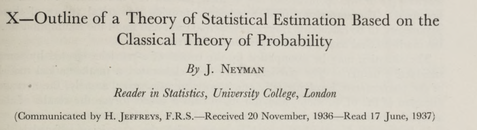
The fallacy article gives the impression that Neyman’s (1936) approach to estimation is outdated and should be replaced with more modern, superior approaches like Bayesian credibility intervals.  For example, they cite Jeffrey’s (1961) theory of probability, which gives the impression that Jeffrey’s work followed Neyman’s work. However, an accurate representation of Neyman’s work reveals that Jeffrey’s work preceded Neyman’s work and that Neyman discussed some of the problems with Jeffrey’s approach in great detail.  Neyman’s critical article was even “communicated” by Jeffreys (these were different times where scientists had open conflict with honor and integrity and actually engaged in scientific debates).

Jeffrey.png

Given that Jeffrey’s approach was published just one year before Neyman’s (1936) article, Neyman’s article probably also offers the first thorough assessment of Jeffrey’s approach. Neyman first gives a thorough account of Jeffrey’s approach (those were the days).

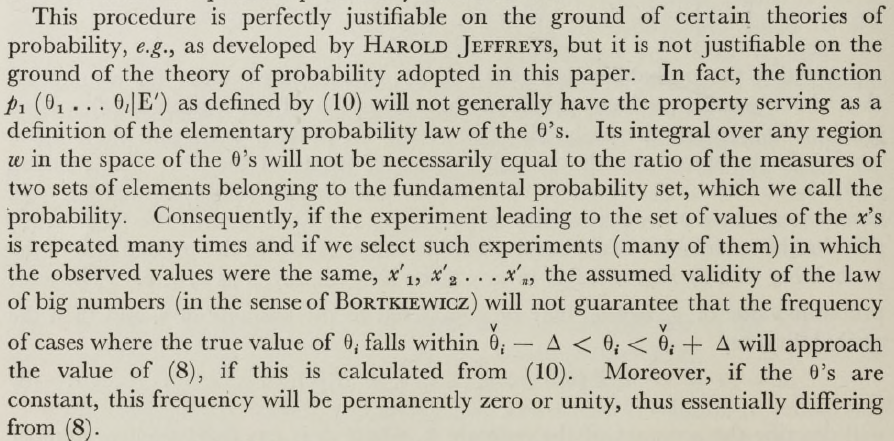
Neyman.png

Neyman then offers his critique of Jeffrey’s approach.

It is known that, as far as we work with the conception of probability as adopted in
this paper, the above theoretically perfect solution may be applied in practice only
in quite exceptional cases, and this for two reasons. 

Importantly, he does not challenge the theory.  He only points out that the theory is not practical because it requires knowledge that is often not available.  That is, to estimate the probability that an unknown parameter is within a specific interval, we need to make prior assumptions about unknown parameters.   This is the problem that has plagued subjective Bayesians approaches.

Neyman then discusses Jeffrey’s approach to solving this problem.  I am not claiming that I am a statistical expert to decide whether Neyman or Jeffrey’s are right. Even statisticians have been unable to resolve these issues and I believe the consensus is that Bayesian credibility intervals and Neyman’s confidence intervals are both mathematically viable approaches to interval estimation with different strengths and weaknesses.

Neyman2.png

I am only trying to point out to unassuming readers of the fallacy article that both approaches are as old as statistics and that the presentation of the issue in this article is biased and violates my personal, and probably idealistic, standards of scientific integrity.   Using a selective quote by Neyman to dismiss confidence intervals and then to omit Neyman’s critic of Bayesian credibility intervals is deceptive and shows an unwillingness or inability to engage in open scientific examination of scientific arguments for and against different estimation methods.

It is sad and ironic that Wagenmakers’ efforts to convert psychologists into Bayesian statisticians is similar to Bem’s (2011) attempt to convert psychologists into believers in parapsychology; or at least in parapsychology as a respectable science. While Bem fudged data to show false empirical evidence, Wagenmakers is misrepresenting the way classic statistics works and ignoring the key problem of Bayesian statistics, namely that Bayesian inferences are contingent on prior assumptions that can be gamed to show what a researcher wants to show.  Wagenmaker used this flexibility in Bayesian statistics to suggest that Bem (2011) presented weak evidence for extra-sensory perception.  However, a rebuttle by Bem showed that Bayesian statistics also showed support for extra-sensory perception with different and more reasonable priors.  Thus, Wagenmakers et al. (2011) were simply wrong to suggest that Bayesian methods would have prevented Bem from providing strong evidence for an incredible phenomenon.

The problem with Bem’s article is not the way he “analyzed” the data. The problem is that Bem violated basic principles of science that are required to draw valid statistical inferences from data.  It would be a miracle if Bayesian methods that assume unbiased data could correct for data falsification.   The problem with Bem’s data has been revealed using statistical tools for the detection of bias (Francis, 2012; Schimmack, 2012, 2015, 2118). There has been no rebuttal from Bem and he admits to the use of practices that invalidate the published p-values.  So, the problem is not the use of p-values, confidence intervals, or Bayesian statistics.  The problem is abuse of statistical methods. There are few cases of abuse of Bayesian methods simply because they are used rarely. However, Bayesian statistics can be gamed without data fudging by specifying convenient priors and failing to inform readers about the effect of priors on results (Gronau et al., 2017).

In conclusion, it is not a fallacy to interpret confidence intervals as a method for interval estimation of unknown parameter estimates. It would be a fallacy to cite Morey et al.’s article as a valid criticism of confidence intervals.  This does not mean that Bayesian credibility intervals are bad or could not be better than confidence intervals. It only means that this article is so blatantly biased and dogmatic that it does not add to the understanding of Neyman’s or Jeffrey’s approach to interval estimation.

P.S.  More discussion of the article can be found on Gelman’s blog.

Andrew Gelman himself comments:

My current favorite (hypothetical) example is an epidemiology study of some small effect where the point estimate of the odds ratio is 3.0 with a 95% conf interval of [1.1, 8.2]. As a 95% confidence interval, this is fine (assuming the underlying assumptions regarding sampling, causal identification, etc. are valid). But if you slap on a flat prior you get a Bayes 95% posterior interval of [1.1, 8.2] which will not in general make sense, because real-world odds ratios are much more likely to be near 1.1 than to be near 8.2. In a practical sense, the uniform prior is causing big problems by introducing the possibility of these high values that are not realistic.

I have to admit some Schadenfreude when I see one Bayesian attacking another Bayesian for the use of an ill-informed prior.  While Bayesians are still fighting over the right priors, practical researchers may be better off to use statistical methods that do not require priors, like, hm, confidence intervals?

P.P.S.  Science requires trust.  At some point, we cannot check all assumptions. I trust Neyman, Cohen, and Muthen and Muthen’s confidence intervals in MPLUS.