Authors: Maria Soto and Ulrich Schimmack
Citation: Soto, M. & Schimmack, U. (2024, June, 24/06/24).  2024 Replicability Report for the Journal 'Evolutionary Psychology'.  Replicability Index.
https://replicationindex.com/2024/06/24/rr24-evopsy/
Introduction
In the 2010s, it became apparent that empirical psychology had a replication problem. When psychologists tested the replicability of 100 results, they found that only 36% of the 97 significant results in original studies could be reproduced (Open Science Collaboration, 2015). In addition, several prominent cases of research fraud further undermined trust in published results. Over the past decade, several proposals were made to improve the credibility of psychology as a science. Replicability Reports aim to improve the credibilty of psychological science by examining the amount of publication bias and the strength of evidence for empirical claims in psychology journals.
The main problem in psychological science is the selective publishing of statistically significant results and the blind trust in statistically significant results as evidence for researchers’ theoretical claims. Unfortunately, psychologists have been unable to self-regulate their behaviour and continue to use unscientific practices to hide evidence that disconfirms their predictions. Moreover, ethical researchers who do not use unscientific practices are at a disadvantage in a game that rewards publishing many articles without concern about these findings’ replicability.
My colleagues and I have developed a statistical tool that can reveal the use of unscientific practices and predict the outcome of replication studies (Brunner & Schimmack, 2021; Bartos & Schimmack, 2022). This method is called z-curve. Z-curve cannot be used to evaluate the credibility of a single study. However, it can provide valuable information about the research practices in a particular research domain.
Replicability-Reports (RR) use z-curve to provide information about psychological journal research and publication practices. This information can aid authors choose journals they want to publish in, provide feedback to journal editors who influence selection bias and replicability of published results, and, most importantly, to readers of these journals.
Evolutionary Psychology
Evolutionary Psychology was founded in 2003. The journal focuses on publishing empirical theoretical and review articles investigating human behaviour from an evolutionary perspective. On average, Evolutionary Psychology publishes about 35 articles in 4 annual issues.
As a whole, evolutionary psychology has produced both highly robust and questionable results. Robust results have been found for sex differences in behaviors and attitudes related to sexuality. Questionable results have been reported for changes in women’s attitudes and behaviors as a function of hormonal changes throughout their menstrual cycle.
According to Web of Science, the impact factor of Evolutionary Psychology ranks 88th in the Experimental Psychology category (Clarivate, 2024). The journal has a 48 H-Index (i.e., 48 articles have received 48 or more citations).
In its lifetime, Evolutionary Psychology has published over 800 articles The average citation rate in this journal is 13.76 citations per article. So far, the journal’s most cited article has been cited 210 times. The article was published in 2008 and investigated the influence of women’s mate value on standards for a long-term mate (Buss & Shackelford, 2008).
The current Editor-in-Chief is Professor Todd K. Shackelford. Additionally, the journal has four other co-editors Dr. Bernhard Fink, Professor Mhairi Gibson, Professor Rose McDermott, and Professor David A. Puts.
Extraction Method
Replication reports are based on automatically extracted test statistics such as F-tests, t-tests, z-tests, and chi2-tests. Additionally, we extracted 95% confidence intervals of odds ratios and regression coefficients. The test statistics were extracted from collected PDF files using a custom R-code. The code relies on the pdftools R package (Ooms, 2024) to render all textboxes from a PDF file into character strings. Once converted the code proceeds to systematically extract the test statistics of interest (Soto & Schimmack, 2024). PDF files identified as editorials, review papers and meta-analyses were excluded. Meta-analyses were excluded to avoid the inclusion of test statistics that were not originally published in Evolution & Human Behavior. Following extraction, the test statistics are converted into absolute z-scores.
Results For All Years
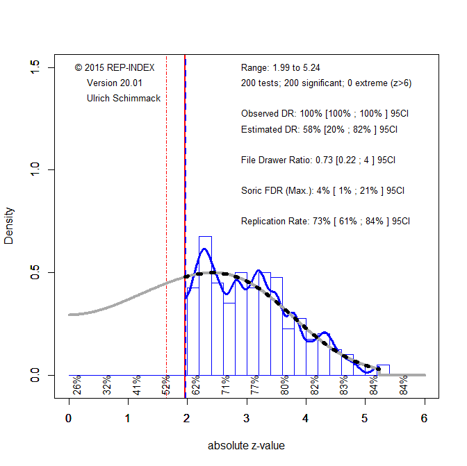
Figure 1 shows a z-curve plot for all articles from 2003-2023 (see Schimmack, 2023, for a detailed description of z-curve plots). However, the total available test statistics available for 2003, 2004 and 2005 were too low to be used individually. Therefore, these years were joined to ensure the plot had enough test statistics for each year. The plot is essentially a histogram of all test statistics converted into absolute z-scores (i.e., the direction of an effect is ignored). Z-scores can be interpreted as the strength of evidence against the null hypothesis that there is no statistical relationship between two variables (i.e., the effect size is zero and the expected z-score is zero). A z-curve plot shows the standard criterion of statistical significance (alpha = .05, z = 1.96) as a vertical red dotted line.

Z-curve plots are limited to values less than z = 6. The reason is that values greater than 6 are so extreme that a successful replication is all but certain unless the value is a computational error or based on fraudulent data. The extreme values are still used for the computation of z-curve statistics but omitted from the plot to highlight the shape of the distribution for diagnostic z-scores in the range from 2 to 6. Using the expectation maximization (EM) algorithm, Z-curve estimates the optimal weights for seven components located at z-values of 0, 1, …. 6 to fit the observed statistically significant z-scores. The predicted distribution is shown as a blue curve. Importantly, the model is fitted to the significant z-scores, but the model predicts the distribution of non-significant results. This makes it possible to examine publication bias (i.e., selective publishing of significant results). Using the estimated distribution of non-significant and significant results, z-curve provides an estimate of the expected discovery rate (EDR); that is, the percentage of significant results that were actually obtained without selection for significance. Using Soric’s (1989) formula the EDR is used to estimate the false discovery risk; that is, the maximum number of significant results that are false positives (i.e., the null-hypothesis is true).
Selection for Significance
The extent of selection bias in a journal can be quantified by comparing the Observed Discovery Rate (ODR) of 68%, 95%CI = 67% to 70% with the Expected Discovery Rate (EDR) of 49%, 95%CI = 26%-63%. The ODR is higher than the upper limit of the confidence interval for the EDR, suggesting the presence of selection for publication. Even though the distance between the ODR and the EDR estimate is narrower than those commonly seen in other journals the present results may underestimate the severity of the problem. This is because the analysis is based on all statistical results. Selection bias is even more problematic for focal hypothesis tests and the ODR for focal tests in psychology journals is often close to 90%.
Expected Replication Rate
The Expected Replication Rate (ERR) estimates the percentage of studies that would produce a significant result again if exact replications with the same sample size were conducted. A comparison of the ERR with the outcome of actual replication studies shows that the ERR is higher than the actual replication rate (Schimmack, 2020). Several factors can explain this discrepancy, such as the difficulty of conducting exact replication studies. Thus, the ERR is an optimist estimate. A conservative estimate is the EDR. The EDR predicts replication outcomes if significance testing does not favour studies with higher power (larger effects and smaller sampling error) because statistical tricks make it just as likely that studies with low power are published. We suggest using the EDR and ERR in combination to estimate the actual replication rate.
The ERR estimate of 72%, 95%CI = 67% to 77%, suggests that the majority of results should produce a statistically significant, p < .05, result again in exact replication studies. However, the EDR of 49% implies that there is some uncertainty about the actual replication rate for studies in this journal and that the success rate can be anywhere between 49% and 72%.
False Positive Risk
The replication crisis has led to concerns that many or even most published results are false positives (i.e., the true effect size is zero). Using Soric’s formula (1989), the maximum false discovery rate can be calculated based on the EDR.
The EDR of 49% implies a False Discovery Risk (FDR) of 6%, 95%CI = 3% to 15%, but the 95%CI of the FDR allows for up to 15% false positive results. This estimate contradicts claims that most published results are false (Ioannidis, 2005).
Changes Over Time
One advantage of automatically extracted test-statistics is that the large number of test statistics makes it possible to examine changes in publication practices over time. We were particularly interested in changes in response to awareness about the replication crisis in recent years.
Z-curve plots for every publication year were calculated to examine time trends through regression analysis. Additionally, the degrees of freedom used in F-tests and t-tests were used as a metric of sample size to observe if these changed over time. Both linear and quadratic trends were considered. The quadratic term was included to observe if any changes occurred in response to the replication crisis. That is, there may have been no changes from 2000 to 2015, but increases in EDR and ERR after 2015.
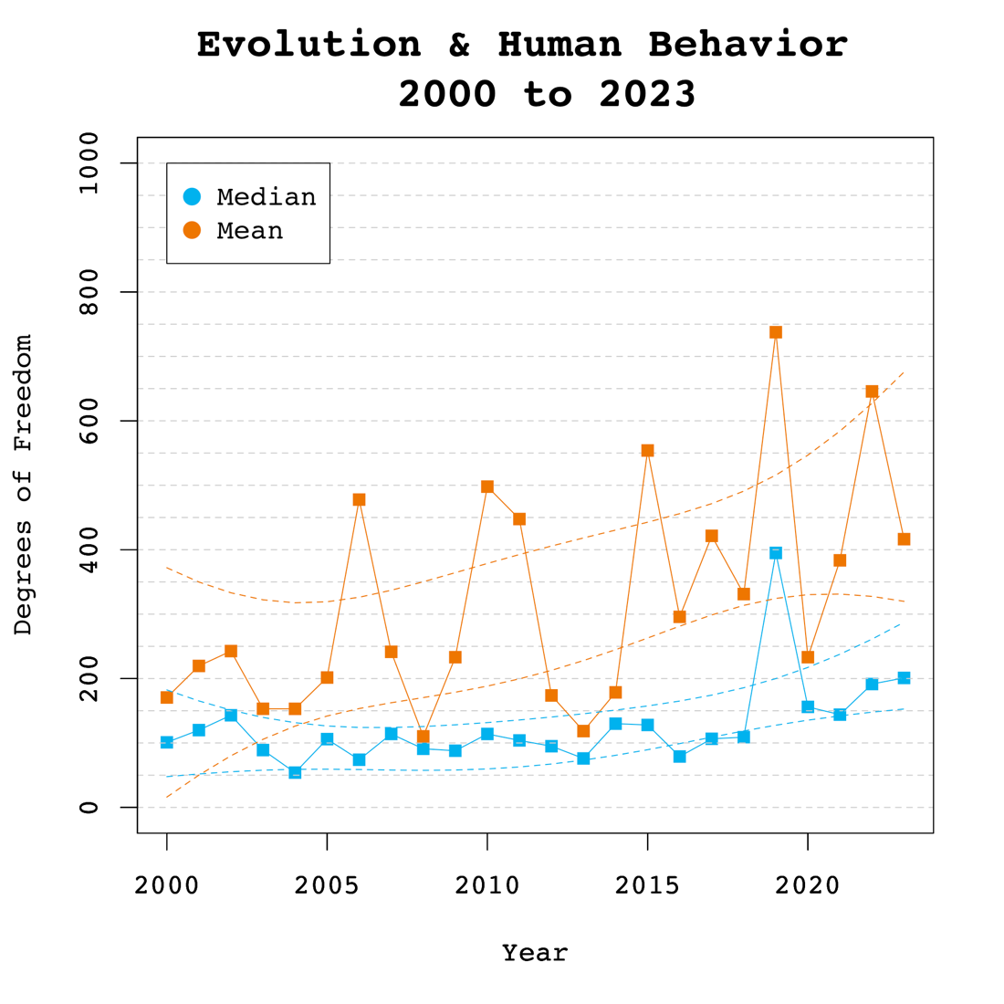
Degrees of Freedom
Figure 2 shows the median and mean degrees of freedom used in F-tests and t-tests reported in Evolutionary Psychology. The mean results are highly variable due to a few studies with extremely large sample sizes. Thus, we focus on the median to examine time trends. The median degrees of freedom over time was 121.54, ranging from 75 to 373. Regression analyses of the median showed a significant linear increase by 6 degrees of freedom per year, b = 6.08, SE = 2.57, p = 0.031. However, there was no evidence that the replication crisis influenced a significant increase in sample sizes as seen by the lack of a significant non-linear trend and a small regression coefficient, b = 0.46, SE = 0.53, p = 0.400.

Observed and Expected Discovery Rates
Figure 3 shows the changes in the ODR and EDR estimates over time. There were no significant linear, b = -0.52 (SE = 0.26 p = 0.063) or non-linear, b = -0.02 (SE = 0.05, p = 0.765) trends observed in the ODR estimate. The regression results for the EDR estimate showed no significant linear, b = -0.66 (SE = 0.64 p = 0.317) or non-linear, b = 0.03 (SE = 0.13 p = 0.847) changes over time. These findings indicate the journal has not increased its publication of non-significant results and continues to report more significant results than one would predict based on the mean power of studies.

Expected Replicability Rates and False Discovery Risks
Figure 4 depicts the false discovery risk (FDR) and the Estimated Replication Rate (ERR). It also shows the Expected Replication Failure rate (EFR = 1 – ERR). A comparison of the EFR with the FDR provides information for the interpretation of replication failures. If the FDR is close to the EFR, many replication failures may be due to false positive results in original studies. In contrast, if the FDR is low, most replication failures will likely be false negative results in underpowered replication studies.
The ERR estimate did not show a significant linear increase over time, b = 0.36, SE = 0.24, p = 0.165. Additionally, no significant non-linear trend was observed, b = -0.03, SE = 0.05, p = 0.523. These findings suggest the increase in sample sizes did not contribute to a statistically significant increase in the power of the published results. These results suggests that replicability of results in this journal has not increased over time and that the results in Figure 1 can be applied to all years.

Visual inspection of Figure 4 depicts the EFR between 30% and 40% and an FDR between 0 and 10%. This suggests that more than half of replication failures are likely to be false negatives in replication studies with the same sample sizes rather than false positive results in the original studies. Studies with large sample sizes and small confidence intervals are needed to distinguish between these two alternative explanations for replication failures.
Adjusting Alpha
A simple solution to a crisis of confidence in published results is to adjust the criterion to reject the null-hypothesis. For example, some researchers have proposed to set alpha to .005 to avoid too many false positive results. With z-curve we can calibrate alpha to keep the false discovery risk at an acceptable level without discarding too many true positive results. To do so, we set alpha to .05, .01, .005, and .001 and examined the false discovery risk.
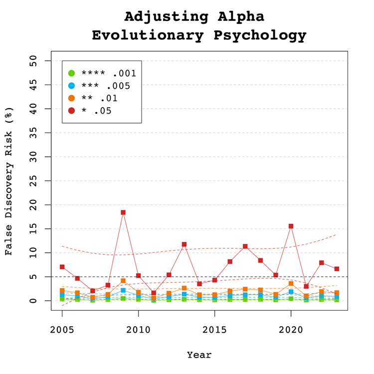
Figure 5 shows that the conventional criterion of p < .05 produces false discovery risks above 5%. The high variability in annual estimates also makes it difficult to provide precise estimates of the FDR. However, adjusting alpha to .01 is sufficient to produce an FDR with tight confidence intervals below 5%. The benefits of reducing alpha further to .005 or .001 are minimal.
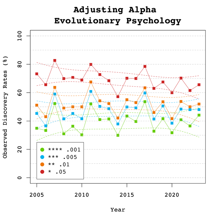
Figure 6 shows the impact of lowering the significance criterion, alpha, on the discovery rate (lower alpha implies fewer significant results). In Evolutionary Psychology lowering alpha to .01 reduces the observed discovery rate by about 20 to 10 percentage points. This implies that 20% of results reported p-values between .05 and .01. These results often have low success rates in actual replication studies (OSC, 2015). Thus, our recommendation is to set alpha to .01 to reduce the false positive risk to 5% and to disregard studies with weak evidence against the null-hypothesis. These studies require actual successful replications with larger samples to provide credible evidence for an evolutionary hypothesis.
There are relatively few studies with p-values between .01 and .005. Thus, more conservative researchers can use alpha = .005 without losing too many additional results.
Limitations
The main limitation of these results is the use of automatically extracted test statistics. This approach cannot distinguish between theoretically important statistical results and other results that are often reported but do not test focal hypotheses (e.g., testing the statistical significance of a manipulation check, reporting a non-significant result for a factor in a complex statistical design that was not expected to produce a significant result).
To examine the influence of automatic extraction on our results, we can compare the results to hand-coding results of over 4,000 hand-coded focal hypotheses in over 40 journals in 2010 and 2020. The ODR was 90% around 2010 and 88% around 2020. Thus, the tendency to report significant results for focal hypothesis tests is even higher than the ODR for all results and there is no indication that this bias has decreased notably over time. The ERR increased a bit from 61% to 67%, but these values are a bit lower than those reported here. Thus, it is possible that focal tests also have lower average power than other tests, but this difference seems to be small. The main finding is that the publishing of non-significant results for focal tests remains an exception in psychology journals and probably also in this journal.
One concern about the publication of our results is that it merely creates a new criterion to game publications. Rather than trying to get p-values below .05, researchers may use tricks to get p-values below .01. However, this argument ignores that it becomes increasingly harder to produce lower p-values with tricks (Simmons et al., 2011). Moreover, z-curve analysis makes it easy to see selection bias for different levels of significance. Thus, a more plausible response to these results is that researchers will increase sample sizes or use other methods to reduce sampling error to increase power.
Conclusion
The replicability report shows that the average power to report a significant result (i.e., a discovery) ranges from 49% to 72% in Evolutionary Psychology. This finding is higher than previous estimates observed in evolutionary psychology journals. However, the confidence intervals are wide and suggest that many published studies remain underpowered. The report did not capture any significant changes over time in the power and replicability as captured by the EDR and the ERR estimates. The false positive risk is modest and can be controlled by setting alpha to .01. Replication attempts of original findings with p-values above .01 should increase sample sizes to produce more conclusive evidence. Lastly, the journal shows clear evidence of selection bias.
There are several ways, the current or future editors of this journal can improve the credibility of results published in this journal. First, results with weak evidence (p-values between .05 and .01) should only be reported as suggestive results that require replication or even request a replication before publication. Second, editors should try to reduce publication bias by prioritizing research questions over results. A well-conducted study with an important question should be published even if the results are not statistically significant. Pre-registration and registered reports can help to reduce publication bias. Editors may also ask for follow-up studies with higher power to follow up on a non-significant result.
Publication bias also implies that point estimates of effect sizes are inflated. It is therefore important to take uncertainty in these estimates into account. Small samples with large sampling errors are usually unable to provide meaningful information about effect sizes and conclusions should be limited to the direction of an effect.
The present results serve as a benchmark for future years to track progress in this journal to ensure trust in research by evolutionary psychologists.