Links to Additional Resources and Answers to Frequently Asked Questions
Chapters
This post is Chapter 1. The R-code for this chapter can be found on my github:
zcurve3.0/Tutorial.R.Script.Chapter1.R at main · UlrichSchimmack/zcurve3.0
(the picture for this post shows a “finger-plot, you can make your own with the code)
Chapter 2 shows the use of z-curve.3.0 with the Open Science Collaboration Reproducibility Project (Science, 2015) p-values of the original studies.
zcurve3.0/Tutorial.R.Script.Chapter2.R at main · UlrichSchimmack/zcurve3.0
Chapter 3 shows the use of z-curve.3.0 with the Open Science Collaboration Reproducibility Project (Science, 2015) p-values of the replication studies.
zcurve3.0/Tutorial.R.Script.Chapter3.R at main · UlrichSchimmack/zcurve3.0
Chapter 4 shows how you can run simulation studies to evaluate the performance of z-curve for yourself.
zcurve3.0/Tutorial.R.Script.Chapter4.R at main · UlrichSchimmack/zcurve3.0
Chapter 5 uses the simulation from Chapter 4 to compare the performance of z-curve with p-curve, another method that aims to estimate the average power of only significant results that is used to estimate the expected replication rate with z-curve.
zcurve3.0/Tutorial.R.Script.Chapter5.R at main · UlrichSchimmack/zcurve3.0
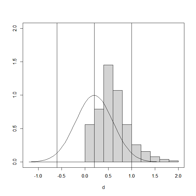
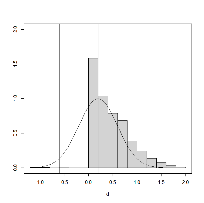
Chapter 6 uses the simulation from Chapter 4 to compare the performance of the default z-curve method with a z-curve that assumes a normal distribution of population effect sizes. The simulation highlights the problem of making distribution assumptions. One of the strengths of z-curve is that it does not make an assumption about the distribution of power.
zcurve3.0/Tutorial.R.Script.Chapter6.R at main · UlrichSchimmack/zcurve3.0
Chapter 7 uses the simulation from Chapter 4 to compare the performance of z-curve to a Bayesian mixture model (bacon). The aim of bacon is different, but it also fits a mixture model to a set of z-values. The simulation results show that z-curve performs better than the Bayesian mixture model.
zcurve3.0/Tutorial.R.Script.Chapter7.R at main · UlrichSchimmack/zcurve3.0
Chapter 8 uses the simulation from Chapter 4 to examine the performance of z-curve with t-values from small studies (N = 30). It introduces a new transformation method that performs better than the default method from z-curve.2.0 and it introduces the t-curve option to analyze t-values from small studies with t-distributions.
zcurve3.0/Tutorial.R.Script.Chapter8.R at main · UlrichSchimmack/zcurve3.0
Chapter 9 simulates p-hacking by combining small samples with favorable trends into a larger sample with a significant result (patchwork samples). The simulation simulates studies with between-subject two-group designs with varying means and SD of effect sizes and sample sizes. It also examines the ability of z-curve to detect p-hacking and compares the performance of the default z-curve that does not make assumptions about the distribution of power and a z-curve model that assumes a normal distribution of power.
zcurve3.0/Tutorial.R.Script.Chapter9.R at main · UlrichSchimmack/zcurve3.0
Brief ChatGPT Generated Summary of Key Points
What Is Z-Curve?
Z-curve is a statistical tool used in meta-analysis, especially for large sets of studies (e.g., more than 100). It can also be used with smaller sets (as few as 10 significant results), but the estimates become less precise.
There are several types of meta-analysis:
- Direct replication: Studies that test the same hypothesis with the same methods.
Example: Several studies testing whether aspirin lowers blood pressure. - Conceptual replication: Studies that test a similar hypothesis using different procedures or measures.
Example: Different studies exploring how stress affects memory using different tasks and memory measures.
In direct replications, we expect low variability in the true effect sizes. In conceptual replications, variability is higher due to different designs.
Z-curve was primarily developed for a third type of meta-analysis: reviewing many studies that ask different questions but share a common feature—like being published in the same journal or during the same time period. In these cases, estimating an average effect size isn’t very meaningful because effects vary so much. Instead, z-curve focuses on statistical integrity, especially the concept of statistical power.
What Is Statistical Power?
I define statistical power as the probability that a study will produce a statistically significant result (usually p < .05).
To understand this, we need to review null hypothesis significance testing (NHST):
- Researchers test a hypothesis (like exercise increasing lifespan) by conducting a study.
- They calculate the effect size (e.g., exercise increase the average lifespan by 2 years) and divide it by the standard error to get a test statistic (e.g., a z-score).
- Higher test-statistics imply a lower probability that the null hypothesis is true. The null hypothesis is that there is no effect. If the probability is below the conventional criterion of 5%, the finding is interpreted as evidence of an effect.
Power is the probability of obtaining a significant result, p < .05.
Hypothetical vs. Observed Power
Textbooks often describe power in hypothetical terms. For example, before collecting data, a researcher might assume an effect size and calculate how many participants are needed for 80% power.
But z-curve does something different. It estimates the average true power of a set of studies. It is only possible to estimate average true power for sets of studies because power estimates based on a single study are typically too imprecise to be useful. Z-curve provides estimates of the average true power of a set of studies and the uncertainty in these estimates.
Populations of Studies
Brunner and Schimmack (2020) introduced an important distinction:
- All studies ever conducted (regardless of whether results were published).
- Only published studies, which are often biased toward significant results.
If we had access to all studies, we could simply calculate power by looking at the proportion of significant results. For example, if 50% of all studies show p < .05, then the average power is 50%.
In reality, we only see a biased sample—mostly significant results that made it into journals. This is called selection bias (or publication bias), and it can mislead us.
What Z-Curve Does
Z-curve helps us correct for this bias by:
- Using the p-values from published studies.
- Converting them to z-scores (e.g., p = .05 → z ≈ 1.96).
- Modeling the distribution of these z-scores to estimate:
- The power of the studies we see,
- The likely number of missing studies,
- And the amount of bias.
Key Terms in Z-Curve
| Term | Meaning |
| ODR (Observed Discovery Rate) | % of studies that report significant results |
| EDR (Expected Discovery Rate) | Estimated % of significant results we’d expect if there were no selection bias |
| ERR (Expected Replication Rate) | Estimated % of significant studies that would replicate if repeated exactly |
| FDR (False Discovery Rate) | Estimated % of significant results that are false positives |
Understanding the Z-Curve Plot
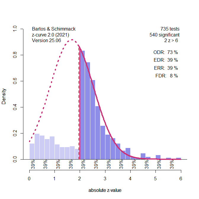
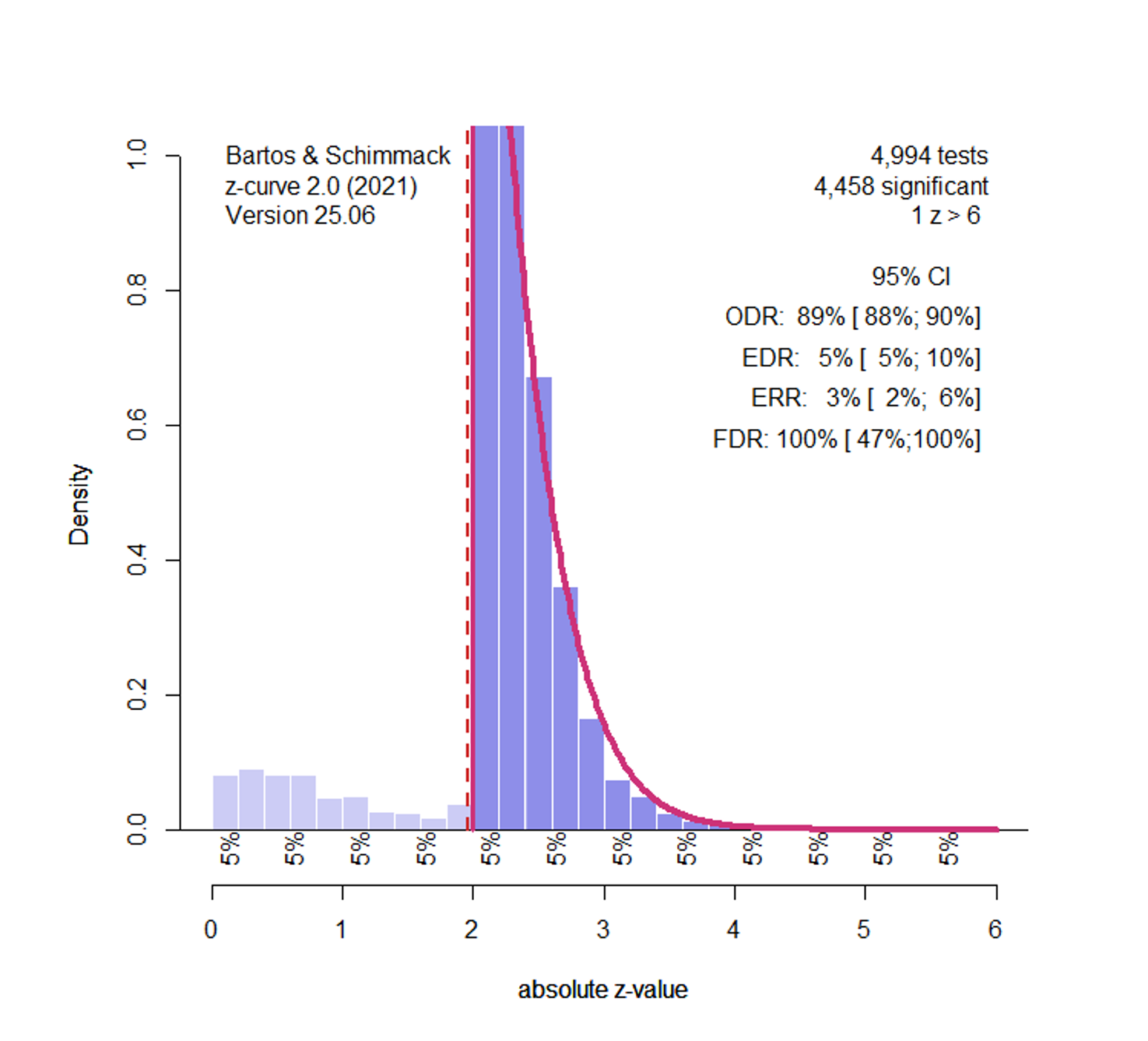
Figure 1. Histogram of z-scores from 1,984 significant tests. The solid red line shows the model’s estimated distribution of observed z-values. The dashed line shows what we’d expect without selection bias. The Observed Discovery Rate (ODR) is 100%, meaning all studies shown are significant. However, the Expected Discovery Rate (EDR) is only 40%, suggesting many non-significant results were omitted. The Expected Replication Rate (ERR) is also 40%, indicating that only 40% of these significant results would likely replicate. The False Discovery Rate (FDR) is estimated at 8%.
Notice how the histogram spikes just above z = 2 (i.e., just significant) and drops off below. This pattern signals selection for significance, which is unlikely to occur due to chance alone.
Homogeneity vs. Heterogeneity of Power
Sometimes all studies in a set have similar power (called homogeneity). In that case, the power of significant and non-significant studies is similar.
However, z-curve allows for heterogeneity, where studies have different power levels. This flexibility makes it better suited to real-world data than methods that assume all studies are equally powered.
When power varies, high-power studies are more likely to produce significant results. That’s why, under heterogeneity, the ERR (for significant studies) is often higher than the EDR (for all studies).
Summary of Key Concepts
- Meta-analysis = Statistical summary of multiple studies.
- Statistical significance = p < .05.
- Power = Probability of finding a significant result.
- Selection bias = Overrepresentation of significant results in the literature.
- ODR = Observed rate of p < .05.
- EDR = Expected rate of p < .05 without bias.
- ERR = Estimated replication success rate of significant results.
Full Introduction
Z-curve is a statistical tool for meta-analysis of larger sets of studies (k > 100). Although it can be used with smaller sets of studies (k > 10 significant results), confidence intervals are likely to be very wide. There are also different types of meta-analysis. The core application of meta-analysis is to combine information from direct replication studies. that is studies that test the same hypothesis (e.g., the effect of aspirin on blood pressure). The most widely used meta-analytic tools aim to estimate the average effect size for a set of studies with the same research question. A second application is to quantitatively review studies on a specific research topic. These studies are called conceptual replication studies. They test the same or related hypothesis, but with different experimental procedures (paradigms). The main difference between meta-analysis of direct and conceptual replication studies is that we would expect less variability in population effect sizes (not the estimates in specific samples) in direct replications, whereas variability is expected to be higher in conceptual replication studies with different experimental manipulations and dependent variables.
Z-curve can be applied to meta-analysis of conceptual replication studies, but it was mainly developed for a third type of meta-analysis. These meta-analyses examine sets of studies with different hypotheses and research designs. Usually, these studies share a common feature. For example, they may be published in the same journal, belong to a specific scientific discipline or sub-discipline, or a specific time period. The main question of interest here is not the average effect size that is likely to vary widely from study to study. The purpose of a z-curve analysis is to examine the credibility or statistical integrity of a set of studies. The term credibility is a broad term that covers many features of a study. Z-curve focuses on statistical power as one criterion for the credibility of a study. To use z-curve and to interpret z-curve results it is therefore important to understand the concept of statistical power. Unfortunately, statistical power is still not part of the standard education in psychology. Thus, I will provide a brief introduction to statistical power.
Statistical Power
Like many other concepts in statistics, statistical power (henceforth power, the only power that does not corrupt), is a probability. To understand power, it is necessary to understand the basics of null-hypothesis significance testing (NHST). When resources are insufficient to estimate effect sizes, researchers often have to settle for the modest goal to examine whether a predicted positive effect (exercise increases longevity) is positive, or a predicted negative effect is negative (asparin lowers blood pressure). The common approach to do so is to estimate the effect size in a sample, estimate the sampling error, compute the ratio of the two, and then compute the probability that the observed effect size or an even bigger one could have been obtained without an effect; that is, a true effect size of 0. Say, the effect of exercise on longevity is an extra 2 years, the sampling error is 1 year, and the test statistic is 2/1 = 2. This value would correspond to a p-value of .05 that the true effect is positive (not 2 years, but greater than 0). P-values below .05 are conventionally used to decide against the null hypothesis and to infer that the true effect size is positive if the estimate is positive or that the true effect is negative if the estimate is negative. Now we can define power. Power is the probability of obtaining a significant result, which typically means a p-value below .05. In short,
Power is the probability of obtaining a statistically significant result.
This definition of power differs from the textbook definition of power because we need to distinguish between different types of powers or power calculations. The most common use of power calculations relies on hypothetical population effect sizes. For example, let’s say we want to conduct a study of exercise and longevity without any prior studies. Therefore, we do not know whether exercise has an effect or how big the effect is. This does not stop us from calculating power because we can just make assumptions about the effect size. Let’s say we assume the effect is two years. The main reason to compute hypothetical power is to plan sample sizes of studies. For example, we have information about the standard deviation of people’s life span and can compute power for hypothetical sample sizes. A common recommendation is to plan studies with 80% power to obtain a significant result with the correct sign.
It would be silly to compute the hypothetical power for an effect size of zero. First, we know that the probability of a significant result without a real effect is set by the research. When they use p < .05 as a rule to determine significance, the probability of obtaining a significant result without a real effect is 5%. If they use p < .01, it is 1%. No calculations are needed. Second, researchers conduct power analysis to find evidence for an effect. So, it would make no sense to do the power calculation with a value of zero. This is null hypothesis that researchers want to reject, and they want a reasonable sample size to do so.
All of this means that hypothetical power calculations assume a non-zero effect size and power is defined as the conditional probability to obtain a significant result for a specified non-zero effect size. Z-curve is used to compute a different type of power. The goal is to estimate the average true power of a set of studies. This average can be made up of a mix of studies in which the null hypothesis is true or false. Therefore, z-curve estimates are no longer conditional on a true effect. When the null hypothesis is true, power is set by the significance criterion. When there is an effect, power is a function of the size of the effect. All of the discussion of conditional probability is just needed to understand the distinction between the definition of power in hypothetical power calculations and in empirical estimates of power with z-curve. The short and simple definition of power is simply the probability of a study to produce a significant result.
Populations of Studies
Brunner and Schimmack (2020) introduce another distinction between power estimates that is important for the understanding of z-curve. One population of studies are all studies that have been conducted independent of the significance criterion. Let’s assume researchers’ computers were hooked up to the internet and whenever they conduct a statistical analysis, the results are stored in a giant database. The database will contain millions of p-values, some above .05 and others below .05. We could now examine the science-wide average power of null hypothesis significance tests. In fact, it would be very easy to do so. Remember, power is defined as the probability to obtain a significant result. We can therefore just compute the percentage of significant results to estimate average power. This is no different than averaging the results of 100,000 roulette games to see how often a table produces “red” or “black” as an outcome. If the table is biased and has more power to get “red” results, you could win a lot of money with that knowledge. In short,
The percentage of significant results in a set of studies provides an estimate of the average power of the set of studies that was conducted.
We would not need a tool like z-curve, if power estimation were that easy. The reason why we need z-curve is that we do not have access to all statistical tests that were conducted in science, psychology, or even a single lab. Although data sharing is becoming more common, we only see a fraction of results that are published in journal articles or preprints on the web. The published set of results is akin to the proverbial tip of the iceberg, and many results remain unreported and are not available for meta-analysis. This means, we only have a sample of studies.
Whenever statisticians draw conclusions about populations from samples, it is necessary to worry about sampling bias. In meta-analyses, this bias is known as publication bias, but a better term for it is selection bias. Scientific journals, especially in psychology, prefer to publish statistically significant results (exercise increases longevity) over non-significant results (exercise may or may not increase longevity). Concerns about selection bias are as old as meta-analyses, but actual meta-analyses have often ignored the risk of selection bias. Z-curve is one of the few tools that can be used to detect selection bias and quantify the amount of selection bias (the other tool is the selection model for effect size estimation).
To examine selection bias, we need a second approach to estimate average power, other than computing the average of significant results. The second approach is to use the exact p-values of a study (e.g., p = .17, .05, .005) and to convert them into z-values (e.g., z = 1, 2, 2.8). These z-values are a function of the true power of a study (e.g., a study with 50% power has an expected z-value of ~ 2), and sampling error. Z-curve uses this information to obtain a second estimate of the average power of a set of studies. If there is no selection bias, the two estimates should be similar, especially in reasonably large sets of studies. However, often the percentage of significant result (power estimate 1) is higher than the z-curve estimate (power estimate 2). This pattern of results suggests selection for significance.
In conclusion, there are two ways to estimate the average power of a set of studies. Without selection bias, the two estimates will be similar. With selection bias, the estimate based on counting significant results will be higher than the estimate based on the exact p-values.
Figure 1 illustrates the extreme scenario that the true power of studies was just 40%, but selection bias filtered out all non-significant results.
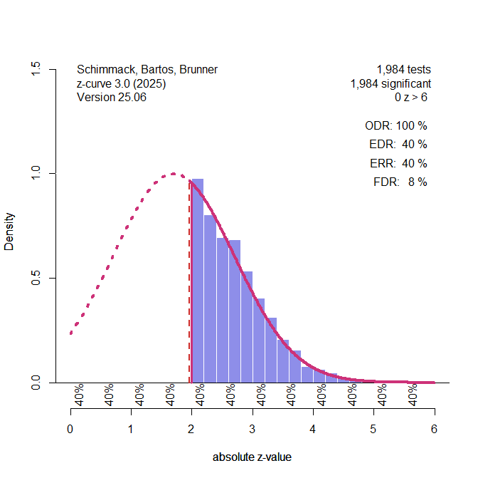
Figure 1. Histogram of z-scores from 1,984 significant tests (based on a simulation of 5,000 studies with 40% power). The solid red line represents the z-curve fit to the distribution of observed z-values. The dashed red line shows the expected distribution without selection bias. The vertical red line shows the significance criterion, p < .05 (two-sided, z ~ 2). ODR = Observed Discovery Rate, EDR = Expected Discovery Rate, ERR = Expected Replication Rate. FDR = False Positive Risk, not relevant for the Introduction.
The figure shows a z-curve plot. Understanding this plot is important for the use of z-curve. First, the plot is a histogram of absolute z-values. Absolute z-values are used because in field-wide meta-analyses the sign has no meaning. In one study, researchers predicted a negative result (aspirin decreases blood pressure) and in another study they predicted a positive result (exercises increases longevity). What matters is that the significant result was used to reject the null hypothesis in either direction. Z-values above 6 are not shown because they are very strong, imply nearly 100% power. The critical range of z-scores are z-scores between 2 (p = .05, just significant) and 4 (~ p = .0001).
The z-curve plot makes it easy to spot selection for significance because there are many studies with just significant results (z > 2) and no studies with just not-significant results that are often called marginally significant results because they are used in publications to reject the null hypothesis with a relaxed criterion. A plot like this cannot be produced by sampling error.
In a z-curve plot, the percentage of significant results is called the observed discovery rate. Discovery is a term used in statistic for a significant result. It does not mean a breaking-news discovery. It just means p < .05. The ODR is 100% because all results are significant. This would imply that all studies tested a true hypothesis with 100% power. However, we know that this is not the case. Z-curve uses the distribution of significant z-scores to estimate power, but there are two populations of power. One population is all studies, including the missing non-significant results. I will explain later how z-curve estimates power. Here it is only important that the estimate is 40%. This estimate is called the expected discovery rate. That is, if we could get access to all missing studies, we would see that only 40% of the studies were significant. Expected therefore means without selection bias and open access to all studies. The difference between the ODR and EDR quantifies the amount of selection bias. Here selection bias inflates the ODR from 40% to 100%.
It is now time to introduce another population of studies. This is the population of studies with significant results. We do not have to assume that all of these studies were published. We just assume that the published studies were not selected based on their p-values. This is a common assumption in selection models. We will see later how changing this assumption can change results.
It is well known that selection introduces bias in averages. Selection for significance, selects studies that had positive sampling error that produced z-scores greater than 2, while the expected z-score without sampling error is only 1.7, not significant on its own. Thus, a simple power calculation for the significant results would overestimate power. Z-curve corrects for this bias and produces an unbiased estimate of the average power of the population of studies with significant results. This estimate of power after selection for significance is called the expected replication rate (ERR). The reason is that average power of the significant results predicts the percentage of significant results if the studies with significant results were replicated exactly, including the same sample sizes. The outcome of this hypothetical replication project would be 40% significant results. The decrease from 100% to 40% is explained by the effect of selection and regression to the mean. A study that had an expected value of 1.7, but sampling error pushed it to 2.1 and produced a significant result is unlikely to have the same sampling error and produce a significant result again.
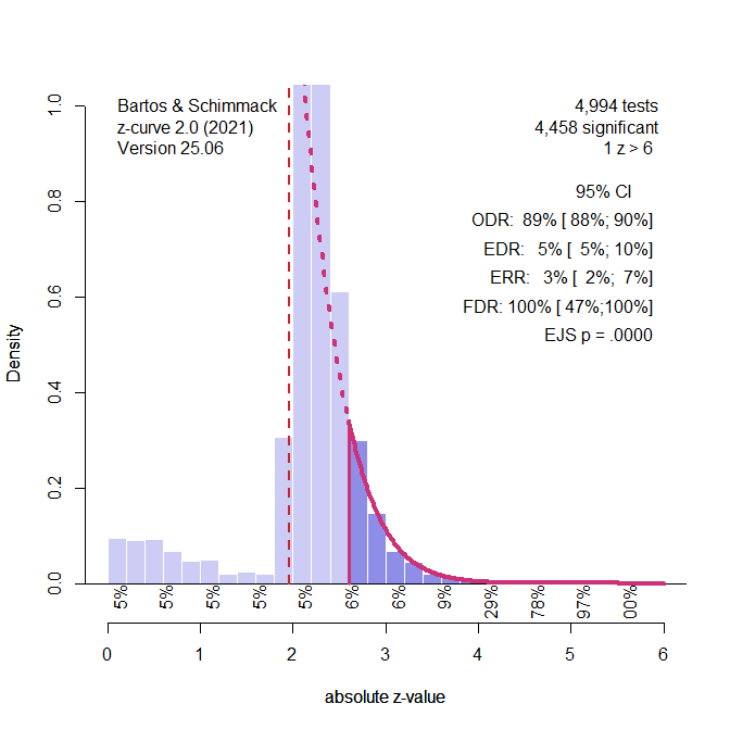
At the bottom of z-curve 3.0, you see estimates of local power. These are average power estimates for ranges of z-values. The default is to use steps of z = .05. You see that the strength of the observed z-values does not matter. Z-values between 0 and 0.5 are estimated to have 40% power as do z-values between 5.5 and 6. This happens when all studies have the same power. When studies differ in power, local power increases because studies with higher power are more likely to produce larger z-values.
When all studies have the same power, power is said to be homogenous. When studies have different levels of power, power is heterogeneous. Homogeneity or small heterogeneity in power imply that it is easy to infer the power of studies with non-significant results from studies with significant results. The reason is that power is more or less the same. Some selection models like p-curve assume homogeneity. For this reason, it is not necessary to distinguish populations of studies with or without significant results. It is assumed that the true power is the same for all studies, and if the true power is the same for all studies, it is also the same for all subsets of studies. This is different for z-curve. Z-curve allows for heterogeneity in power, and z-curve 3.0 provides a test of heterogeneity. If there is heterogeneity in power, the ERR will be higher than the EDR because studies with higher power are more likely to produce a significant result (Brunner & Schimmack, 2020).
To conclude, the introduction introduced basic statistical concepts that are needed to conduct z-curve analyses and to interpret the results correctly. The key constructs are
Meta-Analysis: the statistical analysis of results from multiple studies
Null Hypothesis Significance Testing
Statistical Significance: p < .05 (alpha)
(Statistical) Power: the probability of obtaining a significant result
Conditional Power: the probability of obtaining a significant result with a true effect
Populations of Studies: A set of studies with a common characteristic
Set of all studies: studies with non-significant and significant results
Selection Bias: An overrepresentation of significant results in a set of studies
(Sub)Set of studies with significant results: Subset of studies with p < .05
Observed Discovery Rate (ODR): the percentage of significant results in a set of studies
Expected Discovery Rate (EDR): the z-curve estimate of the discovery rate based on z-values
Expected Replication Rate (ERR): the z-curve estimate of average power for the subset of significant results.