In this series of blog posts, I am reexamining Carter et al.’s (2019) simulation studies that tested various statistical tools to conduct a meta-analysis. The reexamination has three purposes. First, it examines the performance of methods that can detect biases to do so. Second, I examine the ability of methods that estimate heterogeneity to provide good estimates of heterogeneity. Third, I examine the ability of different methods to estimate the average effect size for three different sets of effect sizes, namely (a) the effect size of all studies, including effects in the opposite direction than expected, (b) all positive effect sizes, and (c) all positive and significant effect sizes.
The reason to estimate effect sizes for different sets of studies is that meta-analyses can have different purposes. If all studies are direct replications of each other, we would not want to exclude studies that show negative effects. For example, we want to know that a drug has negative effects in a specific population. However, many meta-analyses in psychology rely on conceptual replications with different interventions and dependent variables. Moreover, many studies are selected to show significant results. In these meta-analyses, the purpose is to find subsets of studies that show the predicted effect with notable effect sizes. In this context, it is not relevant whether researchers tried many other manipulations that did not work. The aim is to find the one’s that did work and studies with significant results are the most likely ones to have real effects. Selection of significance, however, can lead to overestimation of effect sizes and underestimation of heterogeneity. Thus, methods that correct for bias are likely to outperform methods that do not in this setting.
I focus on the selection model implemented in the weightr package in R because it is the only tool that tests for the presence of bias and estimates heterogeneity. I examine the ability of these tests to detect bias when it is present and to provide good estimates of heterogeneity when heterogeneity is present. I also use the model result to compute estimates of the average effect size for all three sets of studies (all, only positive, only positive & significant).
The second method is PET-PEESE because it is widely used. PET-PEESE does not provide conclusive evidence of bias, but a positive relationship between effect sizes and sampling error suggests that bias is present. It does not provide an estimate of heterogeneity. It is also not clear which set of studies are the target of this method. Presumably, it is the average effect size of all studies, but if very few negative results are available, the estimate overestimates this average. I examine whether it produces a more reasonable estimate of the average of the positive results.
P-uniform is included because it is similar to the widely used p-curve method,but has an r-package and produces slightly superior estimates. I am using the LN1MINP method that is less prone to inflated estimates when heterogeneity is present. P-uniform assumes selection bias and provides a test of bias. It does not test heterogeneity. Importantly, p-uniform uses only positive and significant results. It’s performance has to be evaluated against the true average effect size for this subset of studies rather than all studies that are available. It does not provide estimates for the set of only positive results (including non-significant ones) or the set of all studies, including negative results.
Finally, I am using these simulations to examine the performance of z-curve.2.0 (Bartos & Schimmack, 2022). Using exactly the simulations that Carter et al. (2019) used prevents me from simulation hacking; that is, testing situations that show favorable results for my own method. I am testing the performance of z-curve to estimate average power of studies with positive and significant results and the average power of all positive studies. I then use these power estimates to estimate the average effect size for these two sets of studies. I also examine the presence of publication bias and p-hacking with z-curve.
The present blog post, examine the last cell of a 2 x 2 design that varies publication bias and p-hacking. In this post, I examine the condition with high publication bias and no p-hacking (Simulation #392). Like the other simulations (Simulation #296, Simulation #424, Simulation #328), I simulated 100 studies with a small true average population effect size, d = .2, and large heterogeneity, tau = .4. In the other simulations, a properly specified selection model performed well, and no other method performed better. The simulation of selection bias alone without p-hacking should favor models that assume selection bias and correct for it like the selection model, p-uniform, and z-curve. The main challenge for the selection model is that this simulation leaves mostly positive and significant results to be analyzed. Methods like p-uniform and z-curve were designed for scenarios like this. In contrast, the selection model uses information from non-significant results. Thus, it might not perform as well in this simulation.
Simulation
I focus on a sample size of k = 100 studies to examine the properties of confidence intervals with a large, but not unreasonable set of studies. Simulation 392 has the same mean and standard deviation of the true population effect sizes as the other simulations in a 2 x 2 design to explore the effects of publication bias and p-hacking: a small mean effect size of d = .2 and large heterogeneity, tau = 4. The curve in Figure 1 shows the distribution of true population effect sizes. 95% of these effect sizes are in the range from -.6 and 1.

The histogram in Figure 1 shows the distribution of population effect sizes in the studies that are “published,” that is, studies that are available for the meta-analysis. It shows that selection bias changes the population of studies. Selection for significance implies selection for larger effect sizes because studies with larger effect sizes have a higher probability to produce significant results. This means that it is important to distinguish between sets of studies. Should a meta-analysis estimate the original average for all studies, d = .2, only the average of studies with positive results, or the average of studies with positive or significant results?
Figure 2 shows the distribution of the effect size estimates (extreme values below d = 1.2 and above d = 2 are excluded). Selection bias leaves mostly positive results. The presence of some negative results can be explained by the fact that the selection simulation kept negative and statistically significant results.

Histograms of effect sizes do not show the proportion of significant and non-significant results. This can be examined by computing the ratio of effect sizes over sampling error and treat these as approximate z-scores. Alternatively, the sample sizes can be used to compute t-values, and use the corresponding p-values to convert t-values into z-values.
Figure 3 shows the plot of the z-values and the analysis of the z-values with z-curve, using the standard selection model that fits the model to all statistically significant z-values. 103 results with significant negative effects are excluded, leaving 4,897 studies with positive effects. Selection bias leads to an observed discovery rate (ODR, i.e., the percentage of significant positive results) of 91%, while the average true power is estimated at just 42% (it is really 40% based on the true population effect sizes and sample sizes). With 5,000 cases, z-curve can easily show the presence of selection bias because the expected discovery rate predicts at most 54% significant results, when 91% are significant. The figure shows the predicted missing non-significant studies (i.e., the proverbial file-drawer) with the dotted red line.

Z-curve also correctly estimates the average power of the only significant results, which is 66% based on the true population effect sizes of the studies with significant results. In short, a z-curve plot can reveal that the percentage of significant results in a dataset is too high. However, this excess of significant results could be caused by selection bias or p-hacking.
To distinguish selection bias and p-hacking, z-curve can be fitted to only “really” significant results with z-values greater than 2.6. P-hacking would produce more just significant results (2 to 2.6, p = .05 to .01 two-sided) than the model predicts. The results of this test are presented in Figure 4.
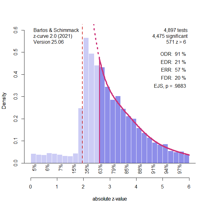
In this particular simulation, there are actually fewer just significant results than the model predicts. The p-value for the binomial test is not significant, p = .9883. As no p-hacking was simulated, this is the correct result (i.e., a true negative result). The simulation study examines the false positive rate of this test when 100 studies are simulated.
Simulation #328 demonstrated that it is difficult to detect and correct for p-hacking with z-curve when it is used. The choice was to accept that p-hacking leads to an underestimation of power as a p-hacking penalty and to use the results of the selection model. Thus, even if a p-hacking test in this simulation would have produced a significant result, it would not change the z-curve model, and the default selection model from Figure 3 was used.
Model Specifications
The specification of the z-curve model was explained and justified above.
The specification of the selection model is easier because it can take selection bias and p-hacking into account in a single model. I used the same approach that I used for the other simulations. I modeled selection bias with the standard approach; that is, a step at .025 (one-tailed) to distinguish positive and significant results from all other results. In addition, I added a step at .005 (one-tailed). This models p-hacking by allowing an excess of p-values between .05 and .01 (two-tailed). The selection weight for this range of p-values is used as a test of p-hacking. In addition, the model had steps at .5 to distinguish positive and negative effects, and .975 to distinguish negative non-significant and negative significant results. The selection weight for positive non-significant results is used as a test of selection bias, but we already saw that p-hacking alone can reduce the amount of non-significant results because these p-hacking moves these p-values into the range of just significant results. Thus, it is difficult to detect selection bias when evidence of p-hacking is present.
The key advantage of the selection model is that it does not rely on significance testing to specify models with or without bias. It will adjust the estimates of the average and standard deviation of the effect sizes based on the estimated amount of bias. The following simulation examines how well this adjustment works when only 100 studies are available to fit the model. .
P-uniform and PET-PEESE do not require thinking and were used as usual.
Selection Model (weightr)
Carter et al. (2019) observe conversion issues with the selection model in some conditions. In my simulation the model produced useable estimates 100% of the time. The test of selection bias showed an average weight for non-significant positive results of .08, average 95%CI = -.02 to .13, and all confidence intervals excluded a value of 1. Thus, the model correctly identified selection bias. The average weight for just significant results was close to 1, average weight = 1.11, average 95%CI = 0.59 to 1.62, and only 1% of the CI did not include a value of 1. Thus, the model correctly identified that bias was produced by selection rather than p-hacking.
Although the model detected selection bias, it did not fully adjust for it. The average effect size estimate for all studies was d = .26, average 95%CI d = .17 to .34, and only 49% of the CI included the true value of d = .20. However, the bias is small. The model also slightly underestimated heterogeneity, average tau = .38, 95% CI = .27 to .46, and only 77% of the confidence intervals included the true value of .40. However, the bias is small.
The estimated effect size for positive results was d = .41, average 95%CI = .29 to .52 and 85% of confidence intervals included the true value of d = .38. The estimated effect size for positive and significant results was d = .57, average 95%CI = .43 to .69, and 93% of the confidence intervals included the true value of d = .58. The performance of the model improves because most studies were positive and significant, and it is easier to estimate the average of studies that are available than to predict averages for sets of studies that are missing.
In short, the performance of the selection model was again good. It correctly distinguished selection and p-hacking and biases in effect size estimates and the estimate of heterogeneity were small. The good performance of the model makes it difficult for other models to do better.
The present results are in line with Carter et al.’s (2019) results based on the default selection model that also performed well in this condition. The key differences are limited to conditions that simulate p-hacking. Thus, the present results merely show that the extension of the model to allow for p-hacking did not reduce the performance of the selection model.
PET-PEESE
PET regresses effect sizes on the corresponding sampling errors. The average estimate was d = .33, average 95%CI = .22 to .43, and only 43% of the confidence intervals included the true parameter, d = .20. Even if this is considered a small bias, the bias is larger than the bias of the selection model. More problematic is that PET is assumed to underestimate true effect sizes, when the estimated effect sizes are positive and significant. In this case, researchers are advised to use PEESE.
PEESE regresses the effect sizes on the sampling variance (i.e., the squared sampling error). PEESE overestimates the true average effect size even more, average d = .42, average 95%CI = .36 to .50, and only 3% of the confidence intervals include the true value.
These findings also confirm Carter et al.’s (2019) findings. “PET-PEESE methods all demonstrated slight increases in upward bias under heterogeneity… In contrast, adding heterogeneity did not increase the bias of the 3PSM estimator” (p. 132). Thus, this is another condition in which the selection model beats PET-PEESE, and PET-PEESE has to demonstrate superior performance in yet unexplored conditions in which it outperforms the selection model.
P-Uniform
P-uniform detected bias in 81% of the simulations. This is lower than the 100% success rate of the selection model. Moreover, the selection model was able to distinguish selection and p-hacking. This makes the selection model a better tool to investigate bias in this simulated scenario.
P-uniform underestimated the average effect size of studies with positive and significant results, average d = .42, average 95%CI = .37 to .47. Only 2% of CI included the true value of d = .58. Thus, p-uniform performs worse than the selection model, even though it is designed for this scenario.
Z-Curve
Z-curve’s primary purpose is to estimate average power, but as shown above, it can be used to examine bias and p-hacking. Z-curve detected bias in 83% of simulation, which is not as good as the performance of the selection model. It also falsely detected p-hacking in 18% of studies, although p-hacking was not used. Thus, the selection model wins.
Consistent with many validation simulations, z-curve’s estimate of average power for positive and significant results that is called the expected replication rate was very good, average ERR = 68%, average 95%CI = 53% to 82%, and the true value of 69% was included in 99% of the confidence intervals.
The average estimate of the average power for the set of positive results (i.e.., the expected discovery rate) was 42%, average 95%CI = .13 to .75, but the confidence interval with only 100 studies is wide. Moreover, only 82% of the confidence intervals included the true value of 40%. Thus, power estimation for the EDR is more uncertain than the nominal 95% confidence intervals suggest.
To compare these results with the selection model, the power estimates can be converted into effect size estimates given the sample sizes of studies with significant results. The average estimate for the set of positive and significant results is d = .52, average 95%CI = .44 to .63, and 81% of the confidence intervals include the true value of d = .58. This is not as good as the estimates from the selection model, average d = .57, average 95%CI = .43 to .69, and 93% of the confidence intervals included the true value of d = .58. Thus, there is no advantage of using z-curve for effect size estimation. The only additional information that it provides is the average power.
For the set of positive results, z-curve effect average size estimate is d = .38, average 95%CI = .16 to .57, and 94% of confidence intervals included the true value of d = .40. While this looks good, it is not better than the performance of the selection model.
Conclusion
The main conclusion from this specific simulation study is that the selection model does well in a simulation with high selection bias. It correctly detects selection bias in all simulations and shows that excessive significant results are produced by selection rather than p-hacking. It slightly overestimates the average effect size for all studies, but it does well in the estimation of the average effect size of all positive studies and all positive and significant studies.
This is the fourth and final simulation of a scenario with 100 studies in the meta-analysis, a small average effect size, d = .2, and large heterogeneity, tau = .4, and the selection model always performed better or as good as other methods. Thus, it remains the model to beat in other scenarios.
It seems unlikely that Carter et al.’s (2019) simulations include conditions that are problematic for the selection model. Namely, it is not clear why milder p-hacking or selection would create problems. It is also not clear why less heterogeneity would be a problem for the model. While I will conduct more replications of Carter et al.’s simulations, I think it is more interesting to examine scenarios that were not included in their design. In their simulations, the selection model benefitted from the simulation of heterogeneity with a normal distribution. This distribution matches the assumption of the selection model. Simulations that change this distribution assumption are needed to really test the robustness of the selection model.
The main preliminary conclusion is that meta-analyses should always include results with a properly specified selection model that allows for (a) different biases for positive and negative results, (b) p-hacking, and (c) overrepresentation of marginally significant results (p < .10, two-sided). Marginally significant results were not modeled here because the simulations did use a strict alpha criterion of .05 to model p-hacking and selection bias. However, in real data, overrepresentation of these results is likely. The proper specification of steps for one-sided p-values is therefore c(.005, .025, .05, .05, .95, .975, 1). Compared to the default model with a single step at .025, this model has 6 more steps and can be called the 9PSM. Some steps can be omitted if a table of the p-value clusters shows zero frequencies, but the model often converges even with zero frequencies and fixes the weight to .01.