In this series of blog posts, I am reexamining Carter et al.’s (2019) simulation studies that tested various statistical tools to conduct meta-analysis. The reexamination has three purposes. First, it examines the performance of methods that can detect biases to do so. Second, I examine the ability of methods that estimate heterogeneity to provide good estimates of heterogeneity. Third, I examine the ability of different methods to estimate the average effect size for three different sets of effect sizes, namely (a) the effect size of all studies, including effects in the opposite direction than expected, (b) all positive effect sizes, and (c) all positive and significant effect sizes.

The reason to estimate effect sizes for different sets of studies is that meta-analyses can have different purposes. If all studies are direct replications of each other, we would not want to exclude studies that show negative effects. For example, we want to know that a drug has negative effects in a specific population. However, many meta-analyses in psychology rely on conceptual replications with different interventions and dependent variables. Moreover, many studies are selected to show significant results. In these meta-analyses, the purpose is to find subsets of studies that show the predicted effect with notable effect sizes. In this context, it is not relevant whether researchers tried many other manipulations that did not work. The aim is to find the one’s that did work and studies with significant results are the most likely ones to have real effects. Selection of significance, however, can lead to overestimation of effect sizes and underestimation of heterogeneity. Thus, methods that correct for bias are likely to outperform methods that do not in this setting.

I focus on the selection model implemented in the weightr package in R because it is the only tool that tests for the presence of bias and estimates heterogeneity. I examine the ability of these tests to detect bias when it is present and to provide good estimates of heterogeneity when heterogeneity is present. I also use the model result to compute estimates of the average effect size for all three sets of studies (all, only positive, only positive & significant).

The second method is PET-PEESE because it is widely used. PET-PEESE does not provide conclusive evidence of bias, but a positive relationship between effect sizes and sampling error suggests that bias is present. It does not provide an estimate of heterogeneity. It is also not clear which set of studies are the target of this method. Presumably, it is the average effect size of all studies, but if very few negative results are available, the estimate overestimates this average. I examine whether it produces a more reasonable estimate of the average of the positive results.

P-uniform is included because it is similar to the widely used p-curve method,but has an r-package and produces slightly superior estimates. I am using the LN1MINP method that is less prone to inflated estimates when heterogeneity is present. P-uniform assumes selection bias and does not test for it. It also does not test heterogeneity. Importantly, p-uniform uses only significant results and estimates the average effect size of the set of studies with positive and significant results. It does not provide estimates for the set of only positive results (including non-significant ones) or the set of all studies, including negative results.

Finally, I am using these simulations to examine the performance of z-curve.2.0. Using exactly the simulations that Carter et al. (2019) used prevents me from simulation hacking; that is, testing situations that show favorable results for my own method. I am testing the performance of z-curve to estimate average power of studies with positive and significant results and the average power of all positive studies. I then use these power estimates to estimate the average effect size for these two sets of studies. I also examine the presence of publication bias and p-hacking with z-curve.

In a simulation without bias I showed that the selection model performs very well (Simulation 296). Here I present a simulation with two sources of bias; selection for significance and p-hacking. This is a plausible scenario for many meta-analyses in psychology, like the ego-depletion literature (Carter et al., 2019).

Simulation 424

I focus on a sample size of k = 100 studies. Many meta-analyses have smaller sets of studies, but some do have 100 studies or more. Fewer studies will mainly lower the power to detect bias and produce wider confidence intervals in estimates. The parameters of 424 for the unbiased model in simulation #296 are an average effect size of d = .2 and large heterogeneity, tau = .4. The curve in Figure 1 shows the distribution of true population effect sizes. 95% of these effect sizes are in the range from -.6 and 1.

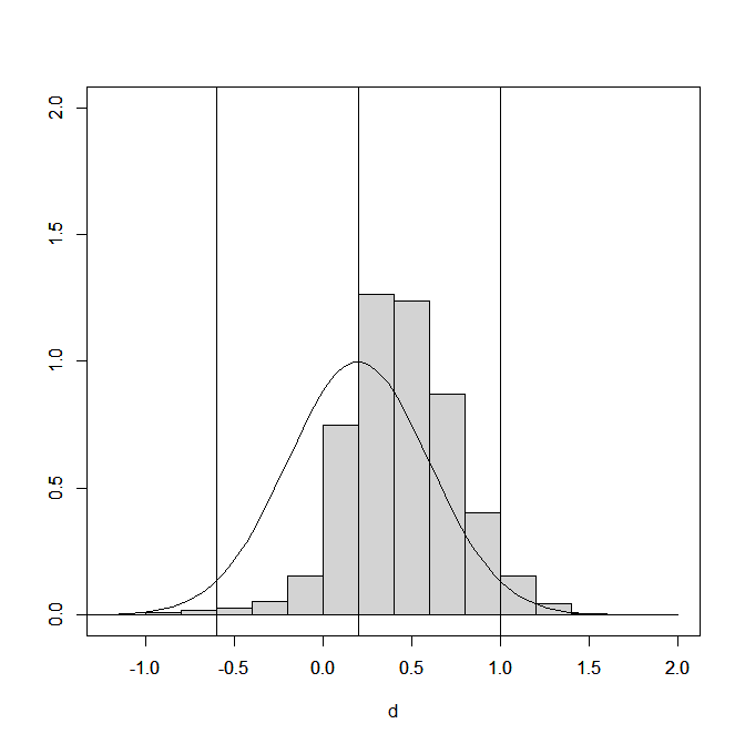
The histogram in Figure 1 shows the distribution of population effect sizes in the studies that are “published,” that is, studies that are available for the meta-analysis. The first question that we have to ask ourselves is which average population effect size we want to estimate. With p-hacking the question is easy. P-hacking produces published studies with inflated effect size estimates, and we want to correct for this bias. With selection bias it is more difficult. Were studies really conducted and are missing or were they never conducted. Were they missing because they had negative effect sizes because something went wrong with the manipulation? When there are hardly any negative results, it may be more interesting to focus on the study that worked. Importantly, worked means studies with a true positive and significant effect, not just studies with a p-value below .05.

Figure 2 shows the distribution of the effect size estimates (extreme values below d = 1.2 and above d = 2 are excluded). The key finding here is that negative results are missing except for a few observations that were selected because they were statistically significant.

Model Specifications

This is an observation that a meta-analyst can observe in their actual data. There are 98 significant negative effects and not a single non-significant negative effect. This is extremely unlikely to occur without selection bias. Thus, we already have evidence of selection against non-significant negative results. Why does this matter. Because selection models are not a magical tool that produce the right answer without thinking about the selection process. Just like confirmatory factor analysis, they require that researchers specify a selection model. Unfortunately, the model comes with some default parameters that allow researchers to get results without thinking. Maybe that option should be disabled to make sure that researchers think. Carter et al. (2019) used the default settings which do not specify selection against non-significant negative results, but not against negative significant results. Not surprisingly, they found that the model underestimated the true population average of d = .2.

Running the default model on these data produced an estimate of d = .00, which is below the true value of d = .20. When the model specifies selection for non-significant results by adding steps at p = .5 and p = .975 (one-tailed), the model correctly notices that these values are missing and the estimated average increases from d = .00 to d = .10.

The model still underestimates the true average. The reason is that the model only assumes selection for significance, while p-hacking was also used to produce too many significant results. To model p-hacking in a selection model, we can specify a range of p-values that are just significant. P-hacking produces too many p-values in this range. I use p-values between .05 and .01 (two-sided) for this purpose. Thus, I added another step at p = .005 (one-tailed).

The estimated average effect size increased to d = .15 and the model correctly showed too many just significant results, selection weight = 2.19, 95%CI = 2.05 to 2.33 (a value of 1 means no bias). The estimate is still lower than the true value, but it is notably closer to the true value than the estimate produced by the mindless default model.

The following simulation examines the performance of the selection model with steps at c=(.005, .025, .5, .975) to examine how the model performs when only 100 studies are available for the analysis.

Z0curve also requires some thinking in the specification of the model. Visual inspection of the data alone would be sufficient to see the presence of selection bias. However, it is also possible to test selection with z-curve by assuming no selection bias. Selection bias and p-hacking will produce too many just significant results. I test for this by comparing the frequency of just significant results (z = 2.0 to 2.4) to the percentage predicted by the z-curve model. When this test is significant, z-curve can be respecified. To distinguish p-hacking and selection bias, the model is estimated using only the observations with z-scores that are clearly significant (z = 2.4) and the test of too-many-just-significant results is repeated. If this test does not produce a significant result, the standard z-curve selection model is fitted with all significant values to get more precise estimates (smaller CI). Evidently, this is less elegant than just fitting a single selection model.

P-uniform and PET-PEESE do not require thinking and were used as usual.

Selection Model (weightr)

Carter et al. (2019) observe conversion issues with the selection model in some conditions. In my simulation the model produced useable estimates 100% of the time. The model showed clear evidence of selection bias. All confidence intervals for the selection weight of non-significant results did not include a value of 1 (no bias). Actually, most of the time the value was fixed to .01 because no non-significant results were present. More importantly, the model also showed evidence of p-hacking. The average selection weight for just significant p-values was 2.37, 95%CI = 0.91 to 3.85. Only 46% of the 95%confidence intervals did not include a value of 1, but power could be increased by using a more liberal significance criterion (many bias tests use alpha = .10). Also, a non-significant result does not imply that there is no p-hacking. Thus, it is still better to specify a model that allows for it even if the parameter is not significantly different from 1.

The average effect size estimate across the simulations was d = .21, average 95%CI = .06 to .36, and 94% of confidence intervals included the true parameter. This is good performance under challenging conditions with selection bias and p-hacking.

This finding is important because this is one condition in which Carter et al.’s ((2019) simulation results suggested that the selection model is biased and cannot be trusted in all conditions. This conclusion is true for the selection model with default specifications, but it is not true for a selection model that accounts for (a) selection against only non-significant results and (b) p-hacking. Thus, the present results undermine Carter et al.’s (2019) influential claim that other methods may outperform the selection model in some conditions. Of course, this is only one condition, but it is a very important one that is likely to be true in many meta-analyses in psychology. Namely, there is high heterogeneity in effect sizes, the average effect size is small, and publication bias and p-hacking are present.

Heterogeneity estimate was underestimated slightly, tau = .35, 95%CI = .18 to .46. Only 73% of confidence intervals included the true parameter of .40. However, the bias is small. How much the bias affects other estimates is examined next.

Based on the mean and heterogeneity estimates, we can compute the average true effect size of all studies with positive results. The true average is d = .37. With the mean and heterogeneity estimates of the selection model, the average estimate is d = .37, 95%CI = .19 to d = .53, and 98% of the confidence intervals included the true parameter.

In this simulation and in some real meta-analysis, p-hacking and selection bias mean that we mostly have only positive and significant results. In this case, we might want to know the true average effect size of the studies that we just analyzed. That is, studies with positive and significant results. To estimate this average I averaged the simulated true population effect sizes of the studies with positive and significant results in the simulation. The value was d = .45.  The average estimate based on the selection model was d = .54, 95%CI = .36 to .73.  88% of the confidence intervals included the true parameter. Thus, the selection model can also be used to estimate the true average effect size for the set of studies with positive and significant results while taking publication bias and p-hacking into account.

To summarize briefly, a properly specified selection model showed evidence of selection for significance and p-hacking and provided good estimates of the true parameters. It is clearly the model to beat for other models to be useful (Brunner & Schimmack, 2020).

PET-PEESE

PET regresses effect sizes on the sampling error. The average estimate was d = .28, 95%CI = .17 to .38, but only 38% of the confidence intervals included the true parameter. Thus, PET is overly confident in its estimates. More problematic is that a positive and significant result is assumed to underestimate the true parameter. In this scenario, effect sizes should be regressed on the square of the sampling error. This model is the PEESE model. The PEESE estimate is d = .40, 95%CI = .33 to .47 and only 8% of the confidence intervals include the true parameter of d = .20.

PET-PEESE also do not provide estimates of heterogeneity that could be used to obtain corrected estimates of the average effect size for the actual population of studies that are available. In this case, the PEESE result is close to the average effect size for the set of positive and significant results, but the method is not designed to estimate this average and it may just be a fluke.

PET-PEESE also do not provide a definitive test of publication bias, although correlations between effect sizes and sampling error suggest that bias is present. It also cannot distinguish between selection bias and p-hacking.

In short, PET-PEESE does nothing that the selection model cannot do and it does a lot less and less well. To justify the use of PET-PEESE or to interpret PET-PEESE results and dismiss selection model results would require a demonstration that PET-PEESE outperforms the selection model in a plausible scenario. Carter et al.’s (2019) simulation #424 is clearly not favoring the PET-PEESE model.

P-Uniform

The p-uniform estimate is d = .32, 95%CI = .21 to .40. It is often stated that p-uniform overestimates effect sizes in the presence of heterogeneity. However, this claim is based on the comparison of p-uniform estimates to the true average for all studies, d = .2. This is not a plausible comparison because p-uniform estimates are based on the subset of significant results and the method estimates the average effect size of this subset. This average is always going to be higher than the overall average when heterogeneity is present. Thus, p-uniform needs to be evaluate as a method that aims to correct for bias in the estimation of the subset of statistically significant and positive results that are used in a p-uniform analysis.

Using the true average effect size for positive and significant results d = .45 as a criterion, p-uniform’s estimates are too low, d = .32, 95%CI = 21 to 40. Only 14% of confidence intervals include the true parameter. This is worse than the performance of the selection model.

P-uniform also provides no estimates of heterogeneity or tests for biases. In short, it does not offer anything in addition to the selection model.

Z-Curve

The main focus of z-curve is on estimation of average power. This is not being estimated by the other methods. It also can be used to detect selection bias. Detecting selection bias is hardly necessary when over 90% of the results are significant, but z-curve correctly showed that there were too many just significant results for a model that assumes no selection for significance, 100% success rate. This matches the performance of the selection model. The more interesting question is whether z-curve can detect p-hacking. The answer is no. Fitting z-curve with “reall” significant results (z > 2.4) led to an average prediction of38% just significant results. The average observed percentage was 41%. Only 27% of the significance tests rejected the null-hypothesis with p < .05. Thus, the selection model is better able to detect p-hacking.

The average true power of studies with positive and significant results was 44%. The average z-curve estimate was 40%, 95%CI = 25% to 56%. 97% of the confidence intervals included the true parameter. This confirms the good performance of z-curve to estimate average power of studies selected for significance in other simulation studies (Brunner & Schimmack, 2020; Bartos & Schimmack, 2022).

The average power of all studies with positive results was 43%. In this case, selection for significance with heterogeneity does not increase average power because p-hacking selects studies with low power. P-hacking also explains why the z-curve estimate is lower than the true power, average 15%, 95%CI = 6% to 37%. Z-curve assumes that just significant results are obtained by running many studies with low power many times. Under this assumption there are many low-powered studies that were not published that drag down the estimate for the average of those studies. However, p-hacking produces just significant results in a single attempt. Thus, there are not many additional studies with low power. One could argue that z-curve punishes researchers for p-hacking, but if the goal is to estimate the true parameter, the selection model is clearly superior.

To compare the z-curve results with the other models, we can use the power estimates and sample sizes of the observed studies to obtain average effect size estimates. For the set of positive and significant results, the estimate is good, d = .44, 95% = .33 to .54, and 96% of the confidence intervals included the true parameter, d = 45. The estimate is clearly superior to the p-uniform estimate. The results in this single simulation are slightly better than the estimates with the selection model, but the difference is not practically significant. Thus, the selection model is the clear winner in this simulation.

Conclusion

The main conclusion from this simulation study is that the selection model outperforms other models. While this is only a single simulation, it is not clear why small quantitative changes to simulated parameters (e.g., k = set of studies, delta = true population average effect size, tau = true heterogeneity) would lead to different conclusions. I will test this prediction in following simulations.

This finding is important because it contradicts Carter et al.’s (2019) finding that the selection model is biased. The reason for these conflicting results is that the selection model requires modeling of the selection process. If the wrong model is specified, the results will be biased, because the assumptions were false, not because the model cannot handle a specific set of data. Carter et al. (2019) specified a model that assumes only selection for significance. This model produces biased results when p-hacking contributes to the overrepresentation of significant results. It also is biased when negative significant results are present. Specifying a selection model that matches the simulation conditions produced good estimates. Importantly, the novel specification of p-hacking with an interval for just significant results showed that p-hacking is present and corrected for it.

It is therefore necessary to revise Carter et al.’s (2019) conclusions about the selection model. The new challenge is to test the correctly specified selection model to examine its robustness across different conditions. The main reason for the good performance of the selection model is that the simulations model heterogeneity with a normal distribution and the selection model assumes normal distribution of population effect sizes. When the true distribution matches the assumed distribution model, it is hard if not impossible to beat the selection model (Brunner & Schimmack, 2020). The main advantage of models like z-curve is that they do not make assumptions about the distribution of population effect sizes or power. Thus, when the distribution is notably different, the selection model may show biases. This hypothesis needs to be tested in future simulation studies. For now, the correctly specified selection model is the clear winner.