Carter et al. (2019): Simulation #392

June 24, 2025UncategorizedUlrich Schimmack

In this series of blog posts, I am reexamining Carter et al.’s (2019) simulation studies that tested various statistical tools to conduct a meta-analysis. The reexamination has three purposes. First, it examines the performance of methods that can detect biases to do so. Second, I examine the ability of methods that estimate heterogeneity to provide good estimates of heterogeneity. Third, I examine the ability of different methods to estimate the average effect size for three different sets of effect sizes, namely (a) the effect size of all studies, including effects in the opposite direction than expected, (b) all positive effect sizes, and (c) all positive and significant effect sizes.

The reason to estimate effect sizes for different sets of studies is that meta-analyses can have different purposes. If all studies are direct replications of each other, we would not want to exclude studies that show negative effects. For example, we want to know that a drug has negative effects in a specific population. However, many meta-analyses in psychology rely on conceptual replications with different interventions and dependent variables. Moreover, many studies are selected to show significant results. In these meta-analyses, the purpose is to find subsets of studies that show the predicted effect with notable effect sizes. In this context, it is not relevant whether researchers tried many other manipulations that did not work. The aim is to find the one’s that did work and studies with significant results are the most likely ones to have real effects. Selection of significance, however, can lead to overestimation of effect sizes and underestimation of heterogeneity. Thus, methods that correct for bias are likely to outperform methods that do not in this setting.

I focus on the selection model implemented in the weightr package in R because it is the only tool that tests for the presence of bias and estimates heterogeneity. I examine the ability of these tests to detect bias when it is present and to provide good estimates of heterogeneity when heterogeneity is present. I also use the model result to compute estimates of the average effect size for all three sets of studies (all, only positive, only positive & significant).

The second method is PET-PEESE because it is widely used. PET-PEESE does not provide conclusive evidence of bias, but a positive relationship between effect sizes and sampling error suggests that bias is present. It does not provide an estimate of heterogeneity. It is also not clear which set of studies are the target of this method. Presumably, it is the average effect size of all studies, but if very few negative results are available, the estimate overestimates this average. I examine whether it produces a more reasonable estimate of the average of the positive results.

P-uniform is included because it is similar to the widely used p-curve method,but has an r-package and produces slightly superior estimates. I am using the LN1MINP method that is less prone to inflated estimates when heterogeneity is present. P-uniform assumes selection bias and provides a test of bias. It does not test heterogeneity. Importantly, p-uniform uses only positive and significant results. It’s performance has to be evaluated against the true average effect size for this subset of studies rather than all studies that are available. It does not provide estimates for the set of only positive results (including non-significant ones) or the set of all studies, including negative results.

Finally, I am using these simulations to examine the performance of z-curve.2.0 (Bartos & Schimmack, 2022). Using exactly the simulations that Carter et al. (2019) used prevents me from simulation hacking; that is, testing situations that show favorable results for my own method. I am testing the performance of z-curve to estimate average power of studies with positive and significant results and the average power of all positive studies. I then use these power estimates to estimate the average effect size for these two sets of studies. I also examine the presence of publication bias and p-hacking with z-curve.

The present blog post, examine the last cell of a 2 x 2 design that varies publication bias and p-hacking. In this post, I examine the condition with high publication bias and no p-hacking (Simulation #392). Like the other simulations (Simulation #296, Simulation #424, Simulation #328), I simulated 100 studies with a small true average population effect size, d = .2, and large heterogeneity, tau = .4. In the other simulations, a properly specified selection model performed well, and no other method performed better. The simulation of selection bias alone without p-hacking should favor models that assume selection bias and correct for it like the selection model, p-uniform, and z-curve. The main challenge for the selection model is that this simulation leaves mostly positive and significant results to be analyzed. Methods like p-uniform and z-curve were designed for scenarios like this. In contrast, the selection model uses information from non-significant results. Thus, it might not perform as well in this simulation.

Simulation

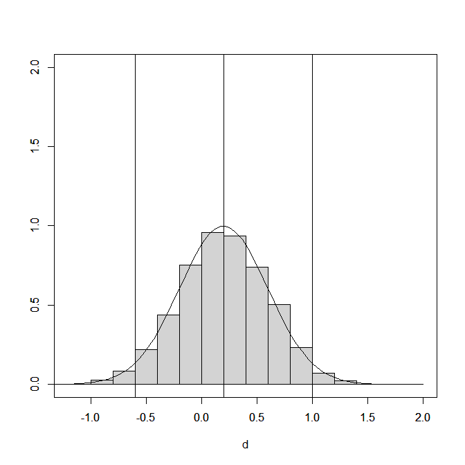
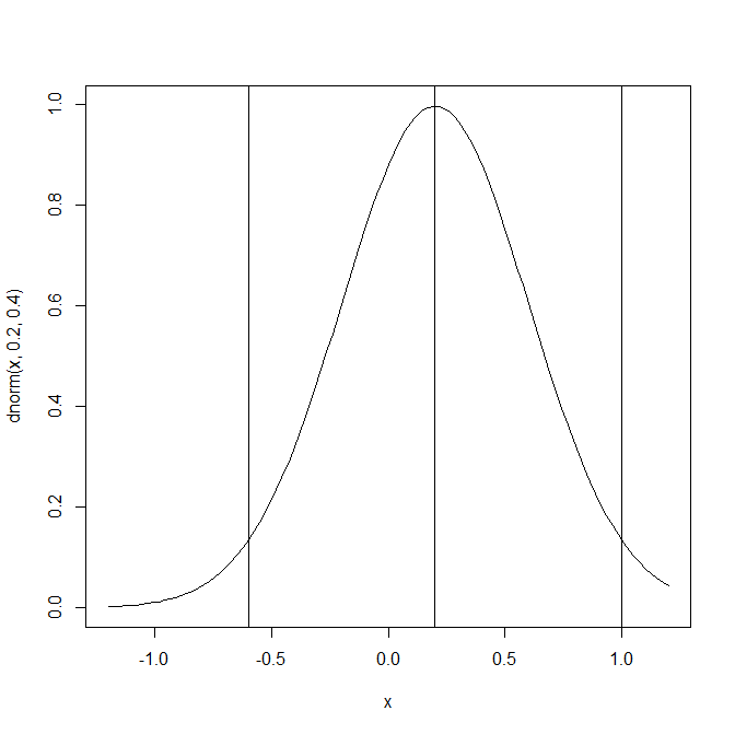
I focus on a sample size of k = 100 studies to examine the properties of confidence intervals with a large, but not unreasonable set of studies. Simulation 392 has the same mean and standard deviation of the true population effect sizes as the other simulations in a 2 x 2 design to explore the effects of publication bias and p-hacking: a small mean effect size of d = .2 and large heterogeneity, tau = 4. The curve in Figure 1 shows the distribution of true population effect sizes. 95% of these effect sizes are in the range from -.6 and 1.

The histogram in Figure 1 shows the distribution of population effect sizes in the studies that are “published,” that is, studies that are available for the meta-analysis. It shows that selection bias changes the population of studies. Selection for significance implies selection for larger effect sizes because studies with larger effect sizes have a higher probability to produce significant results. This means that it is important to distinguish between sets of studies. Should a meta-analysis estimate the original average for all studies, d = .2, only the average of studies with positive results, or the average of studies with positive or significant results?

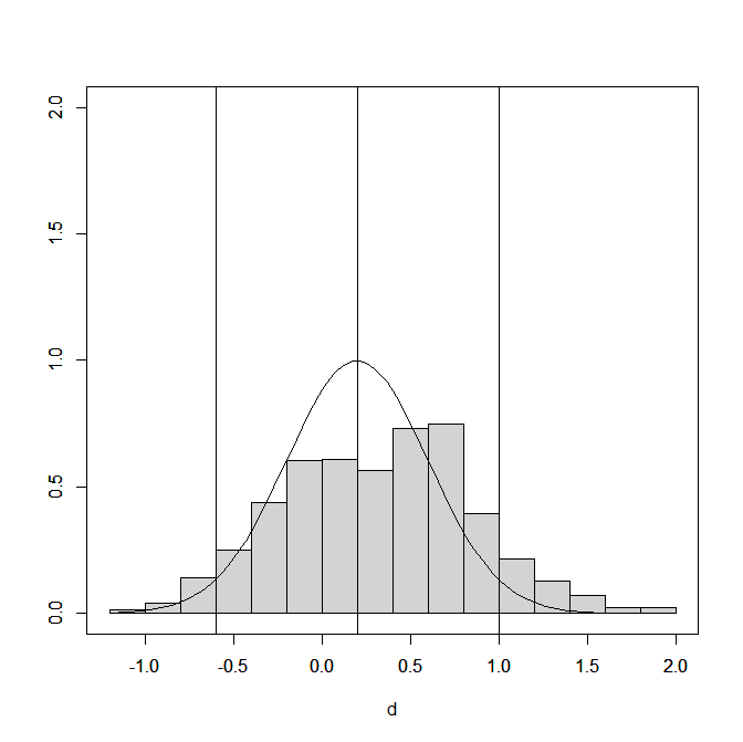
Figure 2 shows the distribution of the effect size estimates (extreme values below d = 1.2 and above d = 2 are excluded). Selection bias leaves mostly positive results. The presence of some negative results can be explained by the fact that the selection simulation kept negative and statistically significant results.

Histograms of effect sizes do not show the proportion of significant and non-significant results. This can be examined by computing the ratio of effect sizes over sampling error and treat these as approximate z-scores. Alternatively, the sample sizes can be used to compute t-values, and use the corresponding p-values to convert t-values into z-values.

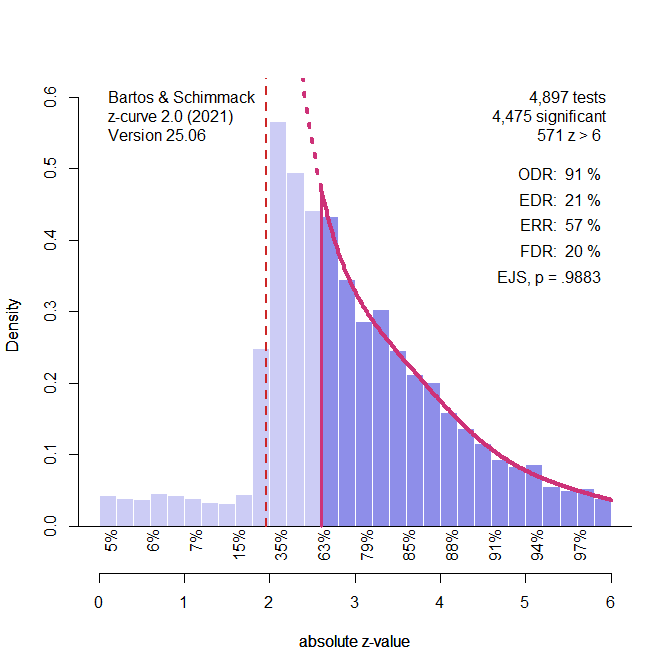
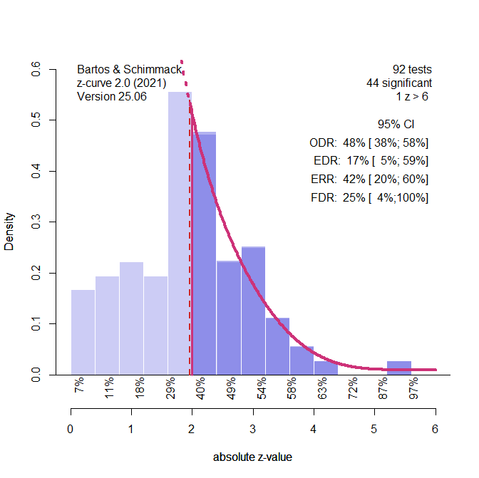
Figure 3 shows the plot of the z-values and the analysis of the z-values with z-curve, using the standard selection model that fits the model to all statistically significant z-values. 103 results with significant negative effects are excluded, leaving 4,897 studies with positive effects. Selection bias leads to an observed discovery rate (ODR, i.e., the percentage of significant positive results) of 91%, while the average true power is estimated at just 42% (it is really 40% based on the true population effect sizes and sample sizes). With 5,000 cases, z-curve can easily show the presence of selection bias because the expected discovery rate predicts at most 54% significant results, when 91% are significant. The figure shows the predicted missing non-significant studies (i.e., the proverbial file-drawer) with the dotted red line.

Z-curve also correctly estimates the average power of the only significant results, which is 66% based on the true population effect sizes of the studies with significant results. In short, a z-curve plot can reveal that the percentage of significant results in a dataset is too high. However, this excess of significant results could be caused by selection bias or p-hacking.

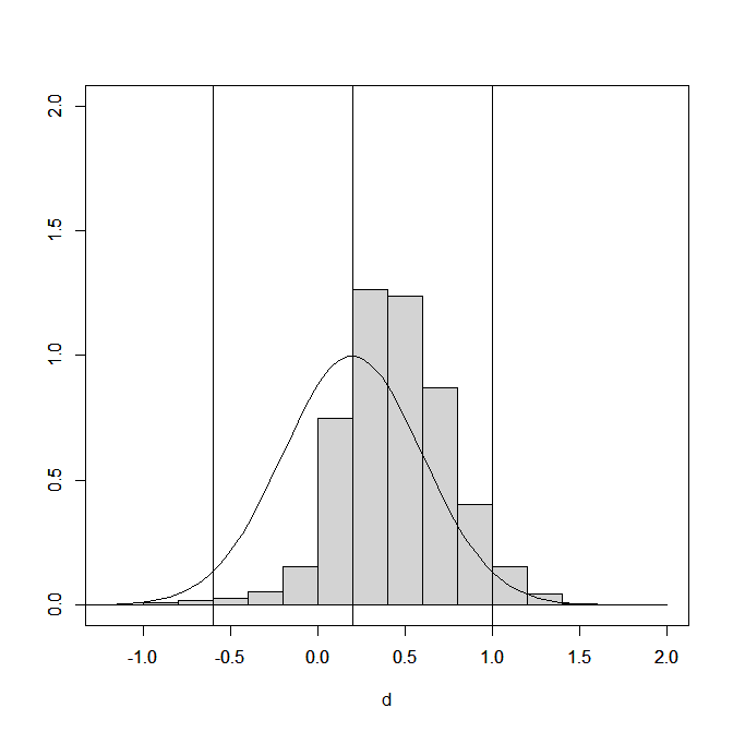
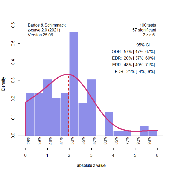
To distinguish selection bias and p-hacking, z-curve can be fitted to only “really” significant results with z-values greater than 2.6. P-hacking would produce more just significant results (2 to 2.6, p = .05 to .01 two-sided) than the model predicts. The results of this test are presented in Figure 4.

In this particular simulation, there are actually fewer just significant results than the model predicts. The p-value for the binomial test is not significant, p = .9883. As no p-hacking was simulated, this is the correct result (i.e., a true negative result). The simulation study examines the false positive rate of this test when 100 studies are simulated.

Simulation #328 demonstrated that it is difficult to detect and correct for p-hacking with z-curve when it is used. The choice was to accept that p-hacking leads to an underestimation of power as a p-hacking penalty and to use the results of the selection model. Thus, even if a p-hacking test in this simulation would have produced a significant result, it would not change the z-curve model, and the default selection model from Figure 3 was used.

Model Specifications

The specification of the z-curve model was explained and justified above.

The specification of the selection model is easier because it can take selection bias and p-hacking into account in a single model. I used the same approach that I used for the other simulations. I modeled selection bias with the standard approach; that is, a step at .025 (one-tailed) to distinguish positive and significant results from all other results. In addition, I added a step at .005 (one-tailed). This models p-hacking by allowing an excess of p-values between .05 and .01 (two-tailed). The selection weight for this range of p-values is used as a test of p-hacking. In addition, the model had steps at .5 to distinguish positive and negative effects, and .975 to distinguish negative non-significant and negative significant results. The selection weight for positive non-significant results is used as a test of selection bias, but we already saw that p-hacking alone can reduce the amount of non-significant results because these p-hacking moves these p-values into the range of just significant results. Thus, it is difficult to detect selection bias when evidence of p-hacking is present.

The key advantage of the selection model is that it does not rely on significance testing to specify models with or without bias. It will adjust the estimates of the average and standard deviation of the effect sizes based on the estimated amount of bias. The following simulation examines how well this adjustment works when only 100 studies are available to fit the model. .

P-uniform and PET-PEESE do not require thinking and were used as usual.

Selection Model (weightr)

Carter et al. (2019) observe conversion issues with the selection model in some conditions. In my simulation the model produced useable estimates 100% of the time. The test of selection bias showed an average weight for non-significant positive results of .08, average 95%CI = -.02 to .13, and all confidence intervals excluded a value of 1. Thus, the model correctly identified selection bias. The average weight for just significant results was close to 1, average weight = 1.11, average 95%CI = 0.59 to 1.62, and only 1% of the CI did not include a value of 1. Thus, the model correctly identified that bias was produced by selection rather than p-hacking.

Although the model detected selection bias, it did not fully adjust for it. The average effect size estimate for all studies was d = .26, average 95%CI d = .17 to .34, and only 49% of the CI included the true value of d = .20. However, the bias is small. The model also slightly underestimated heterogeneity, average tau = .38, 95% CI = .27 to .46, and only 77% of the confidence intervals included the true value of .40. However, the bias is small.

The estimated effect size for positive results was d = .41, average 95%CI = .29 to .52 and 85% of confidence intervals included the true value of d = .38. The estimated effect size for positive and significant results was d = .57, average 95%CI = .43 to .69, and 93% of the confidence intervals included the true value of d = .58. The performance of the model improves because most studies were positive and significant, and it is easier to estimate the average of studies that are available than to predict averages for sets of studies that are missing.

In short, the performance of the selection model was again good. It correctly distinguished selection and p-hacking and biases in effect size estimates and the estimate of heterogeneity were small. The good performance of the model makes it difficult for other models to do better.

The present results are in line with Carter et al.’s (2019) results based on the default selection model that also performed well in this condition. The key differences are limited to conditions that simulate p-hacking. Thus, the present results merely show that the extension of the model to allow for p-hacking did not reduce the performance of the selection model.

PET-PEESE

PET regresses effect sizes on the corresponding sampling errors. The average estimate was d = .33, average 95%CI = .22 to .43, and only 43% of the confidence intervals included the true parameter, d = .20. Even if this is considered a small bias, the bias is larger than the bias of the selection model. More problematic is that PET is assumed to underestimate true effect sizes, when the estimated effect sizes are positive and significant. In this case, researchers are advised to use PEESE.

PEESE regresses the effect sizes on the sampling variance (i.e., the squared sampling error). PEESE overestimates the true average effect size even more, average d = .42, average 95%CI = .36 to .50, and only 3% of the confidence intervals include the true value.

These findings also confirm Carter et al.’s (2019) findings. “PET-PEESE methods all demonstrated slight increases in upward bias under heterogeneity… In contrast, adding heterogeneity did not increase the bias of the 3PSM estimator” (p. 132). Thus, this is another condition in which the selection model beats PET-PEESE, and PET-PEESE has to demonstrate superior performance in yet unexplored conditions in which it outperforms the selection model.

P-Uniform

P-uniform detected bias in 81% of the simulations. This is lower than the 100% success rate of the selection model. Moreover, the selection model was able to distinguish selection and p-hacking. This makes the selection model a better tool to investigate bias in this simulated scenario.

P-uniform underestimated the average effect size of studies with positive and significant results, average d = .42, average 95%CI = .37 to .47. Only 2% of CI included the true value of d = .58. Thus, p-uniform performs worse than the selection model, even though it is designed for this scenario.

Z-Curve

Z-curve’s primary purpose is to estimate average power, but as shown above, it can be used to examine bias and p-hacking. Z-curve detected bias in 83% of simulation, which is not as good as the performance of the selection model. It also falsely detected p-hacking in 18% of studies, although p-hacking was not used. Thus, the selection model wins.

Consistent with many validation simulations, z-curve’s estimate of average power for positive and significant results that is called the expected replication rate was very good, average ERR = 68%, average 95%CI = 53% to 82%, and the true value of 69% was included in 99% of the confidence intervals.

The average estimate of the average power for the set of positive results (i.e.., the expected discovery rate) was 42%, average 95%CI = .13 to .75, but the confidence interval with only 100 studies is wide. Moreover, only 82% of the confidence intervals included the true value of 40%. Thus, power estimation for the EDR is more uncertain than the nominal 95% confidence intervals suggest.

To compare these results with the selection model, the power estimates can be converted into effect size estimates given the sample sizes of studies with significant results. The average estimate for the set of positive and significant results is d = .52, average 95%CI = .44 to .63, and 81% of the confidence intervals include the true value of d = .58. This is not as good as the estimates from the selection model, average d = .57, average 95%CI = .43 to .69, and 93% of the confidence intervals included the true value of d = .58. Thus, there is no advantage of using z-curve for effect size estimation. The only additional information that it provides is the average power.

For the set of positive results, z-curve effect average size estimate is d = .38, average 95%CI = .16 to .57, and 94% of confidence intervals included the true value of d = .40. While this looks good, it is not better than the performance of the selection model.

Conclusion

The main conclusion from this specific simulation study is that the selection model does well in a simulation with high selection bias. It correctly detects selection bias in all simulations and shows that excessive significant results are produced by selection rather than p-hacking. It slightly overestimates the average effect size for all studies, but it does well in the estimation of the average effect size of all positive studies and all positive and significant studies.

This is the fourth and final simulation of a scenario with 100 studies in the meta-analysis, a small average effect size, d = .2, and large heterogeneity, tau = .4, and the selection model always performed better or as good as other methods. Thus, it remains the model to beat in other scenarios.

It seems unlikely that Carter et al.’s (2019) simulations include conditions that are problematic for the selection model. Namely, it is not clear why milder p-hacking or selection would create problems. It is also not clear why less heterogeneity would be a problem for the model. While I will conduct more replications of Carter et al.’s simulations, I think it is more interesting to examine scenarios that were not included in their design. In their simulations, the selection model benefitted from the simulation of heterogeneity with a normal distribution. This distribution matches the assumption of the selection model. Simulations that change this distribution assumption are needed to really test the robustness of the selection model.

The main preliminary conclusion is that meta-analyses should always include results with a properly specified selection model that allows for (a) different biases for positive and negative results, (b) p-hacking, and (c) overrepresentation of marginally significant results (p < .10, two-sided). Marginally significant results were not modeled here because the simulations did use a strict alpha criterion of .05 to model p-hacking and selection bias. However, in real data, overrepresentation of these results is likely. The proper specification of steps for one-sided p-values is therefore c(.005, .025, .05, .05, .95, .975, 1). Compared to the default model with a single step at .025, this model has 6 more steps and can be called the 9PSM. Some steps can be omitted if a table of the p-value clusters shows zero frequencies, but the model often converges even with zero frequencies and fixes the weight to .01.

Carter et al. (2019): Simulation #328

June 23, 2025UncategorizedUlrich Schimmack

P-uniform is included because it is similar to the widely used p-curve method,but has an r-package and produces slightly superior estimates. I am using the LN1MINP method that is less prone to inflated estimates when heterogeneity is present. P-uniform assumes selection bias and does not test for it. It also does not test heterogeneity. Importantly, p-uniform uses only significant results and estimates the average effect size of the set of studies with positive and significant results. It does not provide estimates for the set of only positive results (including non-significant ones) or the set of all studies, including negative results.

Finally, I am using these simulations to examine the performance of z-curve.2.0. Using exactly the simulations that Carter et al. (2019) used prevents me from simulation hacking; that is, testing situations that show favorable results for my own method. I am testing the performance of z-curve to estimate average power of studies with positive and significant results and the average power of all positive studies. I then use these power estimates to estimate the average effect size for these two sets of studies. I also examine the presence of publication bias and p-hacking with z-curve.

In a simulation without bias (Simulation #296) and with high selection bias and p-hacking (Simulation #424) performed well when it properly modeled selection bias and p-hacking. Here I present a simulation that assumes only p-hacking without selection bias (simulation #328). This scenario is interesting because all studies that were conducted are available for the meta-analysis. P-hacking will only inflate effect size estimates for some studies to produce statistical significance. The question is how p-hacking influences effect sizes estimates of models that assume selection bias and correct for selection bias, when selection bias is not present.

Simulation 328

I focus on a sample size of k = 100 studies to examine the properties of confidence intervals with a large, but not unreasonable set of studies. Simulation 328 has the same mean and standard deviation of the true population effect sizes in simulations #296 and #424, namely a small mean effect size of d = .2 and large heterogeneity, tau = 4. The curve in Figure 1 shows the distribution of true population effect sizes. 95% of these effect sizes are in the range from -.6 and 1.

The histogram in Figure 1 shows the distribution of population effect sizes in the studies that are “published,” that is, studies that are available for the meta-analysis. It simply shows that p-hacking does not change the population of studies that are available for meta-analysis. The distribution of the true population effect sizes is not influenced by p-hacking.

Figure 2 shows the distribution of the effect size estimates (extreme values below d = 1.2 and above d = 2 are excluded). The key finding here is that p-hacking moves some observed effect size estimates to the right. Thus, a naive meta-analysis would overestimate the average effect size.

P-hacking however, is a broad term for many practices and it can vary in terms of the amount of bias that is introduced. it is therefore important to examine the amount of p-hacking that is simulated in Carter et al.’s (2019) simulation with “high” p-hacking. The effect of “high” p-hacking on naive meta-analyses is relatively mild.

For the set of all studies, the weighted average effect size estimate is d = .20, not even inflated at all. The reason is that large samples are more likely to produce significant results without p-hacking and are weighted more heavily in the estimation of the true average.

The true average for only positive results is d = .38. The weighted average estimate is d = .44. This is a small bias with little practical consequences.

For the subset of positive and significant results the true average is d = .47. The weighted average estimate is d = .53. Once more, the bias is small.

Thus, Carter et al.’s (2019) simulation of p-hacking in the “high” condition is relatively mild p-hacking. Intense p-hacking would produce 100% significant results without a real effect.

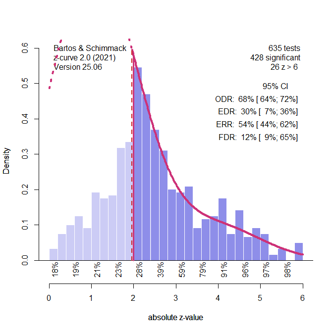
Figure 3 shows the z-curve plot when the effect sizes and sampling errors are converted into z-scores. The distribution of z-scores shows that there are too many just significant results. A binomial test of the frequency of z-scores between 2 and 2.6 (roughly p = .05 to .01, two-sided) shows excessive just significance (EJS) p < .0001. However, these results do not tell us whether the excess is due to publication bias or p-hacking.

To distinguish between the two sources of bias, I fitted the model to the “really” significant results (z > 2.6). This makes it possible to use the EJS test to reveal p-hacking. If the amount of just significant results is not consistent with the model of really significant results, it suggests that p-hacking was used.

The results in Figure 4 show statistically significant excessive just significance, p < .0001, but the model predicts the distribution of just significant z-scores rather well. The difference between observed (54%) and expected (45%) just significant results is small. Thus, the model falsely assumes that selection bias accounts for the high percentage of just significant results. This has important implications for the estimates of power. The average power of the significant results (p < .05, two-sided) is called the Expected Replication Rate and is estimated to be ERR = 43%. This is slightly lower than the true value of 48%. The reason is that p-hacking produces a downward bias and the model does not fully correct for p-hacking.

The effect on the estimate of average power for all positive results, including non-significant ones, is even bigger. This estimate is called the expected discovery rate. The estimate is only 16%, but the true value is 40%. Thus, p-hacking can severely bias the estimate of the EDR when the model assumes selection bias rather than p-hacking contributes to the excess of just significant results.

In actual datasets with fewer studies, it is even more difficult to distinguish between publication bias and p-hacking. So, what can meta-analysts do when there is uncertainty about the cause of excessive just-significant results? First, they can use figures like Figure 3 to examine whether the pattern looks like some non-significant results were moved up to produce an excess of just significant results. In Figure 3, this seems plausible, and we know that this is how the data were created. However, the model in Figure 3 is still influenced by the excessive just significant results and overestimates power. Thus, some correction would be needed. A second option is to fit the normal selection model. This will lead to an underestimation of power, but that can be considered a desirable bias that punishes p-hacking.

Figure 5 shows that the normal selection model underestimates the true power after selection for significance by 10 percentage points (38% versus 48%). This is also not much lower than the estimate with the model that takes p-hacking into account (Figure 4, 43%). Thus, for situations with relatively mild p-hacking like this one, the normal selection model may be acceptable, especially when there is no conclusive evidence that p-hacking was used.

The bias for effect size estimates is also small. The estimate based on the typical selection model for the average effect size of positive and significant results is d = 43, whereas the true parameter is .48. Thus, I used the normal selection model to estimate power and effect sizes for this simulation condition.

To conclude this discussion of p-hacking, it is important to understand the p-hacking simulation in Carter et al.’s (2019) simulation #328. While the condition is the highest level of p-hacking in their design, the amount of p-hacking is mild. First, studies with positive results have an average power of 40% to produce a significant result without p-hacking. Second, about one-quarter of non-significant positive results remain non-significant. Third, many negative results are also available. In contrast, intense p-hacking would produce mostly significant results with less than 33% power (Simonsohn et al. 2014). Thus, additional simulations of p-hacking with more extreme levels of p-hacking are needed to evaluate all methods under those conditions.

Model Specifications

The specification of the z-curve model was explained and justified above.

The specification of the selection model is easier because it can take selection bias and p-hacking into account in a single model. I used the same approach that I used for simulation #424 that simulated selection bias and p-hacking. I modeled selection bias with the standard approach; that is, a step at .025 (one-tailed) to distinguish positive and significant results from all other results. In addition, I added a step at .005 (one-tailed). This models p-hacking by allowing an excess of p-values between .05 and .01 (two-tailed). The selection weight for this range of p-values is used as a test of p-hacking. In addition, the model had steps at .5 to distinguish positive and negative effects, and .975 to distinguish negative non-significant and negative significant results. The selection weight for positive non-significant results is used as a test of selection bias, but we already saw that p-hacking alone can reduce the amount of non-significant results because these p-hacking moves these p-values into the range of just significant results. Thus, it is difficult to detect selection bias when evidence of p-hacking is present.

P-uniform and PET-PEESE do not require thinking and were used as usual.

Selection Model (weightr)

Carter et al. (2019) observe conversion issues with the selection model in some conditions. In my simulation the model produced useable estimates 100% of the time. The test of selection bias showed an average weight for non-significant positive results of .50, but with a wide confidence interval, average CI ranging from -.07 to 1.06. Only 58% of the confidence intervals excluded a value of 1. More important is the test of p-hacking. The average weight for just significant results was high, suggesting p-hacking, w = 3.14. However, the average confidence interval was wide, ranging from .55 to 5.74, and only 11% of the confidence intervals excluded a value of 1. Thus, mild p-hacking is difficult to detect.

The low power to detect p-hacking also led to an underestimation of the average effect size, d = .13, 95%CI = -.13 to .39, but 88% of confidence intervals included the true value of d = .20. The bias is small. The estimate of heterogeneity was close to the true value, tau = .39, average CI = .24 to .49 and 88% of CI included the true value of tau = .40. As a result, the estimate of the subset of results with positive effect size estimates had only a small bias, d = .33, average CI = .05 to .57, and 91% of confidence intervals included the true value of d = .38. Finally, the estimated average for positive and significant results was d = .53, average CI = .23 to .75, and 95% of confidence intervals included the true value of d = .47.

In short, while the selection model was not able to detect p-hacking, it provided good estimates of average effect sizes and heterogeneity in Carter et al.’s (2019) simulation of p-hacking. This finding diverges from Carter et al.’s results that suggested the selection model severely underestimates effect sizes when p-hacking is present. The reason for the discrepancy is that Carter et al. used the default implementation of the selection model that distinguishes only non-significant and significant results. The present results show that a specification that takes p-hacking and the sign of effects into account leads to superior estimates. Thus, Carter et al.’s (2019) concerns about selection models can be addressed with a better specification of the selection model and are not a problem of selection models in general.

It is important that these results were obtained with Carter et al.’s (2019) simulation of p-hacking. Thus, the good results of the selection model cannot be attributed to simulation hacking; that is, I picked a simulation condition that favored a preferred model. Furthermore, my preferred model is z-curve. The good performance of the selection model is just an empirical observation that can be reproduced easily by using the proper specification of the selection model with steps at .005, .025, .050, .500, and .975.

The good performance of the selection model can be explained by Carter et al.’s (2019) simulation of population effect sizes with a normal distribution. This simulation matches the assumptions of the selection model. An interesting question is how the selection model performs with other distributions of effect sizes, but this goes beyond the reexamination of Carter et al.’s (2019) simulation studies.

PET-PEESE

PET regresses effect sizes on the sampling error. The average estimate was d = .04, average 95%CI = -.12 to .21, and only 45% of the confidence intervals included the true parameter, d = .20. Thus, PET often fails to reject the false null-hypothesis. This is a problem because PET does not provide information about heterogeneity. Thus, the non-significant PET result can easily be misinterpreted as evidence that the null hypothesis is true in all studies, which is clearly not the case in this simulation that has high heterogeneity and the set of studies with positive estimates has an average effect size of d = .38.

PEESE regresses the effect sizes on the sampling variance (i.e., the squared sampling error). The average effect size estimate is d = .10, average 95%CI = -.01 to .21, and only 53% of the confidence intervals include the true average for all studies. PEESE is better than PET, but the problem here is that a non-significant estimate for PET is used to favor PET over PEESE estimates.

In short, PET-PEESE is clearly inferior to the selection model in this simulation condition. It was also inferior or not better in the simulation without bias or with p-hacking and selection bias. Whether PET-PEESE ever outperforms the selection model has to be examined in other settings.

P-Uniform

The p-uniform estimate is d = .31, average 95%CI = .12 to .42. It is often stated that p-uniform overestimates effect sizes in the presence of heterogeneity. However, this claim is based on the comparison of p-uniform estimates to the true average for all studies, d = .2. This is not a plausible comparison because p-uniform estimates are based on the subset of significant results and the method estimates the average effect size of this subset. The true average for positive and significant results is d = .38. Thus, p-hacking introduces a small bias. The results are nearly as good as the estimate for positive and significant results with the selection model. Thus, there is no evidence that high heterogeneity inflates p-uniform estimates in this simulation. Rather, p-uniform tends to underestimate the average effect size when p-hacking is used.

P-uniform also tests for the presence of bias, but the test detected bias in only 2% of the studies. The main limitation of p-uniform is that it does not provide tests of heterogeneity. As the selection model estimates average power of positive and significant results as well as p-uniform, and it detects bias better than the p-uniform method, the selection model is superior.

Z-Curve

In a model that assumed no bias, z-curve predicted on average 36% just significant results. On average 54% just significant results were observed, The binomial significance test showed evidence of bias was significant 84% of the time. This shows higher power to detect bias. However, the model that tests specifically for p-hacking found only 25% significant results The reason is that the z-curve prediction of just significant results based on the “really” significant results was close to the observed frequency (49% vs. 54%). Without evidence of p-hacking, the normal selection model was applied to all significant z-scores (z > 1.96).

The average power was estimated at 38%, average 95%CI = 20% to 58%. As the confidence interval is wide, 81% of confidence intervals included the true value of 46%, despite a 10 percentage-point bias. These results show that p-hacking leads to an underestimation of power when just significant results are attributed to selection rather than p-hacking.

The bias is more pronounced for the estimated average power of positive results. Here the average estimate is 16%, average 95%CI = .05 to .43, and none of the confidence intervals included the true value of 40%. This shows that p-hacking can dramatically attenuate estimates of the average power of positive tests. How to deal with this bias will be the topic of future blog posts.

Although the average power of positive and significant results was underestimated, the estimate of the average effect size for this set of results was slightly overestimated, d = .41, average 95%CI = .26 to .55 and 90% of the CI included the true value, d = .38. While this is the best estimate of the average effect size for this set of studies, it is unlikely that this is a robust finding.

The effect size estimate for the set of positive results was underestimated, d = .22, 95% = .00 to .44, and only 66% of confidence intervals included the correct value.

In conclusion, z-curve can provide a powerful test of bias that is more powerful than the test of bias with the selection model. Z-curve also provides useable estimates of average power and effect sizes for the positive and significant results, but the estimates for the set of positive results are severely biased by p-hacking.

Conclusion

The main conclusion from this simulation study is that a properly specified selection model that models p-hacking with overrepresentation of just significant results outperforms other models. This adds to the finding that the selection model performs as well or better than other models without bias or with a mix of selection bias and p-hacking. Z-curve adds information about the presence of bias, either selection or p-hacking, and power estimation for the set of studies with significant results. The other methods have yet to show that they can outperform the selection model in some realistic conditions.

The present results from a reexamination of Carter et al.’s (2019) simulation study are important because the undermine Carter et al.’s (2019) main conclusion that no model works best in all situations. So far, the improved selection model does work well and does not show the strong underestimation of effect sizes that Carter et al. found in this condition with the default selection model (3PSM).

The good performance of the selection model may be due to the modeling of effect sizes with a normal distribution. This helps the selection model because it assumes a normal distribution. It is therefore necessary to expand Carter et al.’s (2019) simulation studies, and model other distributions of population effect sizes. Maybe other methods perform better in those scenarios.

Another observation in this reexamination was that Carter et al.’s high p-hacking condition actually modeled mild p-hacking. It is therefore necessary to examine simulations of more extreme forms of p-hacking.

Carter et al. (2019): Simulation #424

June 19, 2025UncategorizedUlrich Schimmack

In this series of blog posts, I am reexamining Carter et al.’s (2019) simulation studies that tested various statistical tools to conduct meta-analysis. The reexamination has three purposes. First, it examines the performance of methods that can detect biases to do so. Second, I examine the ability of methods that estimate heterogeneity to provide good estimates of heterogeneity. Third, I examine the ability of different methods to estimate the average effect size for three different sets of effect sizes, namely (a) the effect size of all studies, including effects in the opposite direction than expected, (b) all positive effect sizes, and (c) all positive and significant effect sizes.

P-uniform is included because it is similar to the widely used p-curve method,but has an r-package and produces slightly superior estimates. I am using the LN1MINP method that is less prone to inflated estimates when heterogeneity is present. P-uniform assumes selection bias and does not test for it. It also does not test heterogeneity. Importantly, p-uniform uses only significant results and estimates the average effect size of the set of studies with positive and significant results. It does not provide estimates for the set of only positive results (including non-significant ones) or the set of all studies, including negative results.

In a simulation without bias I showed that the selection model performs very well (Simulation 296). Here I present a simulation with two sources of bias; selection for significance and p-hacking. This is a plausible scenario for many meta-analyses in psychology, like the ego-depletion literature (Carter et al., 2019).

Simulation 424

I focus on a sample size of k = 100 studies. Many meta-analyses have smaller sets of studies, but some do have 100 studies or more. Fewer studies will mainly lower the power to detect bias and produce wider confidence intervals in estimates. The parameters of 424 for the unbiased model in simulation #296 are an average effect size of d = .2 and large heterogeneity, tau = .4. The curve in Figure 1 shows the distribution of true population effect sizes. 95% of these effect sizes are in the range from -.6 and 1.

The histogram in Figure 1 shows the distribution of population effect sizes in the studies that are “published,” that is, studies that are available for the meta-analysis. The first question that we have to ask ourselves is which average population effect size we want to estimate. With p-hacking the question is easy. P-hacking produces published studies with inflated effect size estimates, and we want to correct for this bias. With selection bias it is more difficult. Were studies really conducted and are missing or were they never conducted. Were they missing because they had negative effect sizes because something went wrong with the manipulation? When there are hardly any negative results, it may be more interesting to focus on the study that worked. Importantly, worked means studies with a true positive and significant effect, not just studies with a p-value below .05.

Figure 2 shows the distribution of the effect size estimates (extreme values below d = 1.2 and above d = 2 are excluded). The key finding here is that negative results are missing except for a few observations that were selected because they were statistically significant.

Model Specifications

This is an observation that a meta-analyst can observe in their actual data. There are 98 significant negative effects and not a single non-significant negative effect. This is extremely unlikely to occur without selection bias. Thus, we already have evidence of selection against non-significant negative results. Why does this matter. Because selection models are not a magical tool that produce the right answer without thinking about the selection process. Just like confirmatory factor analysis, they require that researchers specify a selection model. Unfortunately, the model comes with some default parameters that allow researchers to get results without thinking. Maybe that option should be disabled to make sure that researchers think. Carter et al. (2019) used the default settings which do not specify selection against non-significant negative results, but not against negative significant results. Not surprisingly, they found that the model underestimated the true population average of d = .2.

Running the default model on these data produced an estimate of d = .00, which is below the true value of d = .20. When the model specifies selection for non-significant results by adding steps at p = .5 and p = .975 (one-tailed), the model correctly notices that these values are missing and the estimated average increases from d = .00 to d = .10.

The model still underestimates the true average. The reason is that the model only assumes selection for significance, while p-hacking was also used to produce too many significant results. To model p-hacking in a selection model, we can specify a range of p-values that are just significant. P-hacking produces too many p-values in this range. I use p-values between .05 and .01 (two-sided) for this purpose. Thus, I added another step at p = .005 (one-tailed).

The estimated average effect size increased to d = .15 and the model correctly showed too many just significant results, selection weight = 2.19, 95%CI = 2.05 to 2.33 (a value of 1 means no bias). The estimate is still lower than the true value, but it is notably closer to the true value than the estimate produced by the mindless default model.

The following simulation examines the performance of the selection model with steps at c=(.005, .025, .5, .975) to examine how the model performs when only 100 studies are available for the analysis.

Z0curve also requires some thinking in the specification of the model. Visual inspection of the data alone would be sufficient to see the presence of selection bias. However, it is also possible to test selection with z-curve by assuming no selection bias. Selection bias and p-hacking will produce too many just significant results. I test for this by comparing the frequency of just significant results (z = 2.0 to 2.4) to the percentage predicted by the z-curve model. When this test is significant, z-curve can be respecified. To distinguish p-hacking and selection bias, the model is estimated using only the observations with z-scores that are clearly significant (z = 2.4) and the test of too-many-just-significant results is repeated. If this test does not produce a significant result, the standard z-curve selection model is fitted with all significant values to get more precise estimates (smaller CI). Evidently, this is less elegant than just fitting a single selection model.

P-uniform and PET-PEESE do not require thinking and were used as usual.

Selection Model (weightr)

Carter et al. (2019) observe conversion issues with the selection model in some conditions. In my simulation the model produced useable estimates 100% of the time. The model showed clear evidence of selection bias. All confidence intervals for the selection weight of non-significant results did not include a value of 1 (no bias). Actually, most of the time the value was fixed to .01 because no non-significant results were present. More importantly, the model also showed evidence of p-hacking. The average selection weight for just significant p-values was 2.37, 95%CI = 0.91 to 3.85. Only 46% of the 95%confidence intervals did not include a value of 1, but power could be increased by using a more liberal significance criterion (many bias tests use alpha = .10). Also, a non-significant result does not imply that there is no p-hacking. Thus, it is still better to specify a model that allows for it even if the parameter is not significantly different from 1.

The average effect size estimate across the simulations was d = .21, average 95%CI = .06 to .36, and 94% of confidence intervals included the true parameter. This is good performance under challenging conditions with selection bias and p-hacking.

This finding is important because this is one condition in which Carter et al.’s ((2019) simulation results suggested that the selection model is biased and cannot be trusted in all conditions. This conclusion is true for the selection model with default specifications, but it is not true for a selection model that accounts for (a) selection against only non-significant results and (b) p-hacking. Thus, the present results undermine Carter et al.’s (2019) influential claim that other methods may outperform the selection model in some conditions. Of course, this is only one condition, but it is a very important one that is likely to be true in many meta-analyses in psychology. Namely, there is high heterogeneity in effect sizes, the average effect size is small, and publication bias and p-hacking are present.

Heterogeneity estimate was underestimated slightly, tau = .35, 95%CI = .18 to .46. Only 73% of confidence intervals included the true parameter of .40. However, the bias is small. How much the bias affects other estimates is examined next.

Based on the mean and heterogeneity estimates, we can compute the average true effect size of all studies with positive results. The true average is d = .37. With the mean and heterogeneity estimates of the selection model, the average estimate is d = .37, 95%CI = .19 to d = .53, and 98% of the confidence intervals included the true parameter.

In this simulation and in some real meta-analysis, p-hacking and selection bias mean that we mostly have only positive and significant results. In this case, we might want to know the true average effect size of the studies that we just analyzed. That is, studies with positive and significant results. To estimate this average I averaged the simulated true population effect sizes of the studies with positive and significant results in the simulation. The value was d = .45. The average estimate based on the selection model was d = .54, 95%CI = .36 to .73. 88% of the confidence intervals included the true parameter. Thus, the selection model can also be used to estimate the true average effect size for the set of studies with positive and significant results while taking publication bias and p-hacking into account.

To summarize briefly, a properly specified selection model showed evidence of selection for significance and p-hacking and provided good estimates of the true parameters. It is clearly the model to beat for other models to be useful (Brunner & Schimmack, 2020).

PET-PEESE

PET regresses effect sizes on the sampling error. The average estimate was d = .28, 95%CI = .17 to .38, but only 38% of the confidence intervals included the true parameter. Thus, PET is overly confident in its estimates. More problematic is that a positive and significant result is assumed to underestimate the true parameter. In this scenario, effect sizes should be regressed on the square of the sampling error. This model is the PEESE model. The PEESE estimate is d = .40, 95%CI = .33 to .47 and only 8% of the confidence intervals include the true parameter of d = .20.

PET-PEESE also do not provide estimates of heterogeneity that could be used to obtain corrected estimates of the average effect size for the actual population of studies that are available. In this case, the PEESE result is close to the average effect size for the set of positive and significant results, but the method is not designed to estimate this average and it may just be a fluke.

PET-PEESE also do not provide a definitive test of publication bias, although correlations between effect sizes and sampling error suggest that bias is present. It also cannot distinguish between selection bias and p-hacking.

In short, PET-PEESE does nothing that the selection model cannot do and it does a lot less and less well. To justify the use of PET-PEESE or to interpret PET-PEESE results and dismiss selection model results would require a demonstration that PET-PEESE outperforms the selection model in a plausible scenario. Carter et al.’s (2019) simulation #424 is clearly not favoring the PET-PEESE model.

P-Uniform

The p-uniform estimate is d = .32, 95%CI = .21 to .40. It is often stated that p-uniform overestimates effect sizes in the presence of heterogeneity. However, this claim is based on the comparison of p-uniform estimates to the true average for all studies, d = .2. This is not a plausible comparison because p-uniform estimates are based on the subset of significant results and the method estimates the average effect size of this subset. This average is always going to be higher than the overall average when heterogeneity is present. Thus, p-uniform needs to be evaluate as a method that aims to correct for bias in the estimation of the subset of statistically significant and positive results that are used in a p-uniform analysis.

Using the true average effect size for positive and significant results d = .45 as a criterion, p-uniform’s estimates are too low, d = .32, 95%CI = 21 to 40. Only 14% of confidence intervals include the true parameter. This is worse than the performance of the selection model.

P-uniform also provides no estimates of heterogeneity or tests for biases. In short, it does not offer anything in addition to the selection model.

Z-Curve

The main focus of z-curve is on estimation of average power. This is not being estimated by the other methods. It also can be used to detect selection bias. Detecting selection bias is hardly necessary when over 90% of the results are significant, but z-curve correctly showed that there were too many just significant results for a model that assumes no selection for significance, 100% success rate. This matches the performance of the selection model. The more interesting question is whether z-curve can detect p-hacking. The answer is no. Fitting z-curve with “reall” significant results (z > 2.4) led to an average prediction of38% just significant results. The average observed percentage was 41%. Only 27% of the significance tests rejected the null-hypothesis with p < .05. Thus, the selection model is better able to detect p-hacking.

The average true power of studies with positive and significant results was 44%. The average z-curve estimate was 40%, 95%CI = 25% to 56%. 97% of the confidence intervals included the true parameter. This confirms the good performance of z-curve to estimate average power of studies selected for significance in other simulation studies (Brunner & Schimmack, 2020; Bartos & Schimmack, 2022).

The average power of all studies with positive results was 43%. In this case, selection for significance with heterogeneity does not increase average power because p-hacking selects studies with low power. P-hacking also explains why the z-curve estimate is lower than the true power, average 15%, 95%CI = 6% to 37%. Z-curve assumes that just significant results are obtained by running many studies with low power many times. Under this assumption there are many low-powered studies that were not published that drag down the estimate for the average of those studies. However, p-hacking produces just significant results in a single attempt. Thus, there are not many additional studies with low power. One could argue that z-curve punishes researchers for p-hacking, but if the goal is to estimate the true parameter, the selection model is clearly superior.

To compare the z-curve results with the other models, we can use the power estimates and sample sizes of the observed studies to obtain average effect size estimates. For the set of positive and significant results, the estimate is good, d = .44, 95% = .33 to .54, and 96% of the confidence intervals included the true parameter, d = 45. The estimate is clearly superior to the p-uniform estimate. The results in this single simulation are slightly better than the estimates with the selection model, but the difference is not practically significant. Thus, the selection model is the clear winner in this simulation.

Conclusion

The main conclusion from this simulation study is that the selection model outperforms other models. While this is only a single simulation, it is not clear why small quantitative changes to simulated parameters (e.g., k = set of studies, delta = true population average effect size, tau = true heterogeneity) would lead to different conclusions. I will test this prediction in following simulations.

This finding is important because it contradicts Carter et al.’s (2019) finding that the selection model is biased. The reason for these conflicting results is that the selection model requires modeling of the selection process. If the wrong model is specified, the results will be biased, because the assumptions were false, not because the model cannot handle a specific set of data. Carter et al. (2019) specified a model that assumes only selection for significance. This model produces biased results when p-hacking contributes to the overrepresentation of significant results. It also is biased when negative significant results are present. Specifying a selection model that matches the simulation conditions produced good estimates. Importantly, the novel specification of p-hacking with an interval for just significant results showed that p-hacking is present and corrected for it.

It is therefore necessary to revise Carter et al.’s (2019) conclusions about the selection model. The new challenge is to test the correctly specified selection model to examine its robustness across different conditions. The main reason for the good performance of the selection model is that the simulations model heterogeneity with a normal distribution and the selection model assumes normal distribution of population effect sizes. When the true distribution matches the assumed distribution model, it is hard if not impossible to beat the selection model (Brunner & Schimmack, 2020). The main advantage of models like z-curve is that they do not make assumptions about the distribution of population effect sizes or power. Thus, when the distribution is notably different, the selection model may show biases. This hypothesis needs to be tested in future simulation studies. For now, the correctly specified selection model is the clear winner.

Carter et al. (2019): Simulation #296

June 18, 2025UncategorizedUlrich Schimmack

P-uniform is included because it is similar to the widely used p-curve method,but has an r-package and produces slightly superior estimates. I am using the LN1MINP method that is less prone to inflated estimates when heterogeneity is present. P-uniform assumes selection bias and does not test for it. It also does not test heterogeneity. Importantly, p-uniform uses only significant results and estimates the average effect size of the set of studies with positive and significant results. It does not provide estimates for the set of only positive results (including non-significant ones) or the set of all studies, including negative results.

Simulation 296

The first simulation examines how the methods perform when no biases are present. For bias tests, this condition examines the false positive risk. With alpha = .05 or 95%confidence intervals, bias should be detected in no more than 5 out of 100 simulations.

The key parameters of this simulation are an average effect size of d = .2 and large heterogeneity, tau = .4. This simulation assumes that 95% of effect sizes are in the range from -.6 to 1 and that most effect sizes are small. The percentage of results with a negative sign in this simulation is a bit implausible, but it helps to see the differences between the three sets of studies.

The average effect size for all studies is of course d = .2. Selecting only positive results produces an average effect size of d = .38. The set of positive results with significant results depends on the sample sizes of the studies. Sample sizes in the Carter et al. (2017) simulation varied widely from N = 10 to N = 3124 with a mean of N = 134 and a median of N = 52. Running a large simulation produced a rate of 9% significant results with a negative sign and 24% significant results with a positive sign. The power of producing a significant result for only the positive results was 38%. The average effect size for studies with positive and significant results was d = .57. Thus, this simulation implies that expected significant results are obtained with strong effect sizes that are stronger than most actual effect sizes in psychology.

Selection Model (weightr)

Carter et al. (2019) observe conversion issues with the selection model in some conditions. In this simulation, no problems were encountered. The estimated effect size for all studies was d = .19, average 95%CI .04 to .35. 93% of the CI included the true value of .20. I consider this an acceptable performance. The estimated heterogeneity was close to the true value, tau = .39, average 95%CI = .28 to ..47, but coverage was a bit lower than the 95%CI suggests, 88%. Based on these mean and tau estimates, I computed an effect size estimate for the positive results of d = .37, average 95%CI = .18 to .53, 96% coverage. This is also a good performance. The estimated mean for the positive and significant results was d = .57, average 95%CI = .36 to .73 with 96% coverage.

Selection for significance would produce too few non-significant results. This is tested with the selection weight for p-values between .025 (one-sided) and 1. A value of 1 implies no selection bias. The average estimate was 1.16, average 95%CI = .04 to 2.28. 87% of confidence intervals included the true value. The other 13% showed false evidence of selection bias.

To test for p-hacking, I specified a model with a step at p = .005 (one-sided). The model then computes a weight for the proportion of p-values in the range between .025 (one-sided) and .005 (one-sided) that corresponds to two-sided p-values between .01 and .05. P-hacking would produce too many significant results in this range. The weight for p-values between .01 and .05 (two-sided) was 1.19, average 95%CI = .08 to 2.30. 91% of CIs included a value of 1, indicating no evidence of p-hacking. The other CIs produced values less than 1. Thus, none of the confidence intervals suggested p-hacking.

In sum, the selection model performed flawlessly in this condition.

PET-PEESE

PET regresses effect sizes on the sampling error. The average estimate was close to the average for all studies, d = .19, 95%CI = .05 to .33. However, only 62% of confidence intervals included the true value. When PET produces a positive and significant result, it is recommended to run a second regression with the variance (sampling error squared) as predictor. This is called the PEESE model. In the absence of any bias, the results are practically the same.

In this specific condition, the selection model is clearly preferable to the PET-PEESE approach. First, it produces more accurate estimates of the average effect size (better coverage of the confidence interval). Second, it produces an estimate of heterogeneity that can be used to compute averages for subsets of studies with positive results or positive and significant results. Third, it tests for the presence of bias and can provide evidence that bias is not present or small. In this case, it is also possible to run normal meta-analytic models, but the results would be no different from the selection model. The only reason to use PET-PEESE would be that the model performs better in other situations, when the selection model fails (Carter et al., 2019).

P-Uniform

The p-uniform estimate is d = .42, 95%CI = .31 to .50. It is often stated that p-uniform overestimates effect sizes in the presence of heterogeneity. However, this claim is based on the comparison of p-uniform estimates to the true average for all studies, d = .2. This is not a plausible comparison because p-uniform estimates are based on the subset of significant results and the method estimates the average effect size of this subset. This average is always going to be higher than the overall average when heterogeneity is present. What is more disturbing is that the p-uniform method is not even able to estimate the average effect size of the positive and significant results correctly. Compared to the true average of d = .57, the estimate is too low and only 25% of the confidence intervals include the true value. P-uniform also does not provide information about the presence of bias or estimate heterogeneity. In short, the method fails in this specific condition.

Z-Curve

The estimated average power of positive and significant results was 66%, 95%CI = 58% to 73%. All confidence intervals included the true value. This overperformance is explained by the conservative confidence intervals implemented in z-curve. The average power before selection for significance was estimated to be 40%, 95%CI = 31% to 48%. The coverage was 100%. Based on the average power of studies selected for significance, z-curve estimated an average effect size of d = .56, 95%CI = .46 to .68. The 95%CI included the true parameter 92% of the time. This is clearly better than p-uniform, but not better than the selection model that also provides information about heterogeneity in effect sizes. The estimate for the average effect size for all positive results (based on the estimated power before selection for significance) was d = .40; 95%CI = .31 to .50 with 91% coverage. This is not a bad performance, but the selection model did better.

To test for bias, the model compared the observed percentage of z-values between 2.0 and 2.4 with the predicted percentage of just significant results in this range. The average observed percentage was 23.4%. The average predicted percentage was 23.0%. Only 3% of the significance tests showed false evidence of bias with alpha = .05. Thus, the test has the intended error rate.

Conclusion

Based on this single condition from Carter et al.’s (2019) meta-analysis, the selection model is clearly superior to all other models. It provides information about the presence of bias and heterogeneity and it provides good estimates and confidence intervals for the estimates of the overall average and heterogeneity. These values can be used to get good estimates of the average effect size for subsets of studies with only positive results or only positive and significant results.

The information about heterogeneity is particularly important. An estimate of tau = .4 shows large heterogeneity. It is implausible that such big differences could be observed in a meta-analysis of direct replication studies. Evidence of such large heterogeneity should trigger a careful examination of the data to see whether coding mistakes or other errors produced unexpected heterogeneity.

Large heterogeneity, however, is to be expected in psychological meta-analysis that combine apples, oranges, grapes, and other fruits in one salad. In these ‘fruit-salad’ meta-analyses, the overall effect size is meaningless and easily misinterpreted. For example, with a median effect size of N = 52 and an average effect size of d = .2, a study has virtually no power to detect an effect. This might lead to the conclusion that the entire literature is underpowered. However, an analysis of the subset of studies with positive and significant results shows an effect size of d = .57 that can be detected even with small samples of N = 52. A focus on the subset of studies with positive and significant results would produce a tasty salad of studies that can be replicated. This was the idea behind p-curve, but p-curve and p-uniform are not the best tools to look for tasty fruit. As noted by McShane et al., selection models can do a better job.

If you found this post interesting, you probably want to know how the selection model (and other models) perform when selection bias and p-hacking produce too many significant results. Well, stay tuned for the next post that examines p-hacking.

P-Curve Does Not Detect P-Hacking: What Does?

June 15, 2025UncategorizedUlrich Schimmack

The early 2010s were a time of upheaval in psychological science. Many psychologists lost faith in the ability of significance testing to test psychological theories. Until then, the common concern was that many studies often were doomed to failure because low statistical power was bound to produce a non-significant result. By the same logic, a significant result was assumed to be a sure sign of a real effect. This logical fallacy ignored that psychology journals nearly always report successful rejections of null hypotheses. This selection for significance in published results renders statistically significance insignificant (Sterling, 1959). In the worst-case scenario, every published significant result is the result of many attempts without a real effect (Rosenthal, 1979).

An influential article by Simmons, Nelson, and Simonsohn (2011) showed that researchers may not need to try very often to get a significant result. Using a number of statistical tricks, known as questionable research practices or p-hacking, it is possible to get a significant result in every other study without a real effect. Ample evidence shows that publication bias and p-hacking contribute to the high success rate in psychological journals (Francis, 2012; Schimmack, 2012). The observed discovery rates (i.e., the percentage of significant results) is simply too high, given the true probability of studies to produce significant results.

For the diagnosis of excessive significance, it is irrelevant whether bias is produced by the omission of non-significant results or p-hacking; that is the use of statistical tricks to turn a non-significant result into a significant one. Both selection for significance and p-hacking undermine the purpose of meta-analyses to estimate the true population effect size. Several methods have been developed to correct for bias in meta-analyses. For the purpose of bias correction, however, it is important whether selection or p-hacking produced too many significant results (Carter et al., 2019). It is therefore important to distinguish between selection bias and p-hacking in meta-analyses that correct for bias.

P-Curve

Simonsohn, Nelson, and Simmons (2014) developed a statistical method called p-curve. The basic idea of p-curve is that p-values have a uniform distribution when the null-hypothesis is true. This is also true for the distribution of the p-values below .05 that are typically used to reject the null-hypothesis. Thus, if only significant results are available, which is often the case in psychology journals, the distribution of p-values can be used to test the null-hypothesis that all significant results are false positive results (i..e., the null hypothesis is true in all studies). In this case, the p-value distribution is uniform. A variety of tests have been developed to test this null hypothesis. The specifics of these tests are not relevant here.

The p-curve authors have pointed out that many p-hacking methods will produce an abnormal distribution of p-values that is biased towards weak evidence (i.e., more p-values above .01 than below .01). They call this a right-skewed distribution. So far, this test is the only direct test of p-hacking in actual data. The key problem with this test is that it only works when the null hypothesis is true in all studies and the evidence was produced with p-hacking. If the null hypothesis is false and the studies produced significant results with an effect, the method fails because true effects produce more p-values below .01. This is a problem because p-hacking still inflates effect size estimates in meta-analyses. Here I show alternative ways to diagnose p-hacking when the null-hypothesis is false that can be used to correct for p-hacking in meta-analyses.

Effect of P-Hacking on Meta-Analyses

Carter et al. (2019) conducted an extensive simulation study to examine the influence of p-hacking and publication bias on effect size estimates using a variety of meta-analytic methods. One of the more promising approaches to correct for bias are selection models (McShane, Böckenholt, & Hansen, 2016). Selection models can assume homogeneity of the population effect size (i.e., all studies have the same population effect size) or heterogeneity (i.e., different studies have different population effect sizes). The heterogeneous model assumes that population effect sizes are normally distributed and estimates the standard deviation of this distribution (tau). More importantly, the selection model allows for bias. To do so, researchers can specify ranges of p-values that have the same probability of being published. A simple model distinguishes between significant results in favor of a specific hypothesis (p < .025 one-tailed) and all other results (p > .025, one-tailed). Other specifications are possible and more plausible. For example, it is easy to find studies with p-values just above .05 (two-sided) that are used to reject the null-hypothesis. These, marginally significant results are more likely to be published than results that clearly do not support a hypothesis. This can be specified with a model with steps at .025 and .05 (one-sided). It is also possible that researchers select for the direction of an effect, even if the effects are not significant. This can be tested with another step at p = .5 (one-sided) that distinguishes between positive, p < .50 and negative p > .50 results.

The key problem of selection models is that they assume selection for significance rather than p-hacking. The following example shows how this assumption influences the results and that p-hacking results in an underestimation of effect sizes. As these problems are a bigger concern when power is low so that more p-hacking is needed to get significant results, and when heterogeneity is relatively high. Heterogeneity cannot be too high because large effect sizes produce high power.

I used Carter et al.’s simulation with high p-hacking. I set the mean of the population effect sizes to zero with a wide standard deviation of tau = .4. I simulated 1,000 studies for large sample accuracy that reveals systematic biases in the methods.

I used the weightr package in R to fit the selection model to the data. I first specified the standard model that assumes only selection for significance at p = .025, one-tailed. The key results are the estimates of the average effect size, d = -.21, 95%CI = -.24 to -.18. This shows that p-hacking leads to underestimation of the average effect size when bias is assumed to be caused by selection for significance. Heterogeneity was also underestimated, but only slightly, tau = .30, 95%CI = .28 to .32.

To model p-hacking, I added a step at p = .005 (one-tailed). The rational is that p-hacking produces more just significant results than a model without bias would predict. To capture this prediction, I am using p-values between .05 and .01, two-sided. First of all, the model correctly notices that just significant p-values are overrepresented, selection weight = 2.77 (nearly 3 times as many as p-values below .01 that have no selection bias). This shows that the specification of a step at .005 (one-tailed) can be used to diagnose p-hacking.

However, adding this step did not produce unbiased estimates. The average was still underestimated, d = -.14, 95%CI = -.19 to -.09. However, the estimate of heterogeneity was better and no longer significantly different from the true value, tau = .38, 95%CI = .34 to .41.

These results are encouraging and suggest that the performance of selection models can be improved by distinguishing between selection for significance and p-hacking and to use the prevalence of p-values between .05 and .01 to diagnose p-hacking.

To verify that selection does not produce too many just-significant results, I simulated data without bias and then deleted 50% of the non-significant results. The model still slightly underestimated the true average, d = -.08, 95%CI = -.13 to -.03, but it estimated heterogeneity correctly, tau = .42, 95%CI = .39 to .46. It also correctly diagnosed that about half of the non-significant results were missing, selection weight = 60%, 95%CI = 41% to 78%.

Importantly, adding a step at p = .005 (one-tailed) did not change these results. The model correctly noted no special selection for just significant results, selection weight = 1.11, 95%CI = .71 to 1.51. The average was still slightly underestimated, d = -.07, 95%CI -.13 to -.02. Heterogeneity was estimated the same as in the model without the extra step, tau = .43, 95%CI = .39 to .47.

What if only significant results are available?

The previous simulation included positive and negative non-significant results. However, in reality, most results are positive and significant. I therefore examined the performance of the selection model under conditions that led to the development of p-curve.

I used the same simulation of p-hacking, but selected only statistically significant positive results. Before I present the results, it is important to discuss the performance criterion that should be used to evaluate the model. As noted by Simonsohn et al. (2018), when only positive and significant results are available, and results are heterogeneous, we want to know the true effect size of studies that have been published; not the hypothetical effect size of studies that may even have produced negative results. Moreover, selection models cannot estimate the average for a hypothetical set of studies with negative results if there are no negative results. I therefore computed the mean and standard deviation of the simulated population effect sizes in the set of studies with positive results as the criterion values. The values were mean d = .26 and sd = .28.

The default model that only assumes selection for significance produced an estimate of d = .18, 95%CI = .15 to .22. The estimate of heterogeneity is tau = .15, 95%CI = .12 to .16. The model that specified p-hacking with a step at p = .005 (one-tailed) showed evidence of p-hacking, selection weight = 3.60, 95%CI = 2.36 to 4.84. The estimated average increased to d = .29, 95%CI = .24 to .35, and the estimate of heterogeneity was also higher, tau = .20, 95%CI = .16 to .24.

These results show that selection models do not require non-significant results and can diagnose and correct for p-hacking even if only positive significant results are available.

Conclusion

It is well-established that psychology journals publish too many statistically significant results. This bias has been attributed to publication bias or p-hacking. While publication bias and p-hacking both inflate effect sizes estimates with methods that do not correct for bias, they have different effects on methods that aim to correct for bias. Traditional specifications of selection models assume selection bias and do not take p-hacking into account. This leads to underestimation of the average effect size and heterogeneity. Here I presented a solution to this problem. P-hacking tends to produce just-significant results. Thus, p-hacking can be diagnosed by specifying a range of p-values between .05 and .01 (two-sided). Rather than selection, we are expecting overrepresentation (eights > 1) for this bin of p-values. I confirmed this prediction with a few simulation studies and showed that a model with a step at .005 produces better estimates of the average and heterogeneity of population effect sizes. This even works when only positive and significant results are available. The ability of selection models to estimate averages and heterogeneity, while taking different biases into account, makes these models very attractive for effect size meta-analysis. The key drawback of other methods (p-curve, p-uniform, PET-PEESE) is that they do not provide information about the amount of heterogeneity. The main problem of traditional meta-analytic methods is that they overestimate the average and heterogeneity when bias is present. The inclusion of an extra step to model p-hacking may further improve the performance of this model.

The estimated average effect size is d = .42, 95%CI = .33 to .51. This is close to the true value and the true value is included in the 95% confidence interval. The model also has a higher estimate of heterogeneity, tau = .20, 95%CI = .00 to .30, but the 95%CI still includes a value of zero and the model fails to reject the false null-hypothesis of heterogeneity.

P-uniform is similar to p-curve (McShane et al., 2016). I used p-uniform because p-curve does not have an r-package. I used the LN1MINP method because it shows better performance than the LNP method that tends to overestimate effect sizes and did not fit the data as well in the diagnostic plot for these data. The p-uniform estimate was d = .35, 95%CI = .26 to .44. This result shows underestimation of the true average, but the 95%CI includes the true parameter and the difference is not practically significant. Thus, p-hacking

Karsten T. Hansen

, including p-curve and a very similar method called p-uniform.

Here

However, several statistical tools try to correct for bias in observed data to evaluate a specific literatue.

Assumption Checking Prevents Assumption Hacking in Multiverse Meta-Analyses

June 13, 2025UncategorizedUlrich Schimmack

In a nutshell

Statistical methods for meta-analyses make different assumptions. For this reason, different methods can produce different results with the same data. Meta-analysts often struggle to make sense of these inconsistent results. A simple solution to this problem is to test testable assumptions. Key assumptions that influence results are publication bias and heterogeneity of population effect sizes. Here I show how testing these assumptions explains inconsistencies in results and that methods that violate assumptions produce biased results. I also show with two examples (ego-depletion, terror management) and tailored simulation studies that different methods produce similar results when the same data are used. Differences in results in the terror management multiverse meta-analysis were found to be due to the analysis of different datasets. The article clarifies many misconceptions about multiverse meta-analysis and helps applied researchers and readers to make sense of these studies.

Introduction

Meta-analysis is nearly as old as inferential statistics itself. Genius and eugenicist Sir Fisher developed the first meta-analysis using p-values rather than effect sizes. He also developed the first bias test for meta-analysis and showed that Mendal’s famous data of dominant and recessive genes in peas were too good to be statistically true. In this case, of course, the main finding remained true.

Effect size meta-analysis emerged in the 1960s to make sense of conflicting results in original studies with small sample sizes that lacked statistical power to detect small to moderate effects in a single study (Cohen, 1962).

When we can assume that the available data are an unbiased sample and all studies estimate the same population effect size, it is rather simple to meta-analyze the data. A simple average of effect sizes will do. A better solution is to weigh the data by sample size or similar weights (inverse of sampling error, inverse of sampling variance). Voila, you have the best estimate of the population effect size.

In reality, meta-analytic results can produce dramatically false results for two reasons. First, effect sizes may vary across studies due to a number of factors. For example, effects (or statistical relationships in correlational studies) can vary across populations. Variability in effect sizes is called heterogeneity. Hundreds of articles have discussed the problem of heterogeneity and how to deal with it in meta-analyses.

The second problem is that existing studies may be biased towards evidence for an effect. For example, a meta-analysis of extrasensory perception suggested that it is real. This is known as publication bias. Standard meta-analysis will overestimate effect sizes when publication bias is present. For example, the Open Science Collaboration Reproducibility Project (2015) showed that a naive meta-analysis of psychological studies would overestimate effect sizes by 100%. If a meta-analysis of diets suggests that the average weight loss is 50ls, the real effect is only 25lb. Even more dramatic examples can be found. A naive meta-analysis of ego-depletion (loss of willpower) suggested an effect of .6 standard deviations. A bias-corrected meta-analysis and credible replication studies suggest that the effect may not exist or is very small (< .1 standard deviations); an inflation by 600%.

During the credibility revolution, interest in statistical methods that can detect and correct for publication bias has increased tremendously. To ensure robustness of results, it is often recommended to use multiple methods (Carter et al., 2019). The use of multiple methods to test robustness has become known as a multiverse analysis. Unfortunately, multiverse meta-analyses often produce inconsistent results. As a result, meta-analytic articles often produce no clear conclusions (Cheng et al., 2025).

In this article, I argue that lack of robustness is to be expected because different meta-analytic models make different assumptions. Although it is widely acknowledged that valid statistical inferences require valid assumptions, testing of assumptions is often ignored (Nimon, 2012). This is also true for multiverse meta-analyses. Even when methods test assumptions, the results of this tests are often ignored (Carter et al., 2010; Cheng et al., 2025). In this article, I illustrate with simulations and two actual datasets how testing of assumptions resolves seemingly inconsistent effect size estimates. Some of these inconsistent results are based on false assumptions and are invalid because sound inferences require valid assumptions.

However, untested assumptions are not the only reason for inconsistent results. I show two additional problems in multiverse meta-analyses. First, sometimes models are mis-specified when default assumptions do not fit a dataset (Cheng et al., 2025). Second, sometimes the input data for different methods differ substantially and lead to different conclusions (Cheng et al., 2025).

I use the results from Carter et al.’s (2019) multiverse meta-analysis for educational purposes. The data are from a real dataset with 116 ego-depletion studies. The results in their Table 2 showed that different methods produced different average effect size estimates that “would lead to different conclusions” (p. 139). As can be seen in the table, the average effect size estimates range from -.27 standardized mean differences (SMD), a small negative effect, to an SDM of .55, a strong effect. Subsequently, I show that this large range of estimates is not as inconsistent as it seems to be. Rather, the results are all consistent with (a) the presence of publication bias, (b) the presence of heterogeneity, and (c) a moderate to strong effect for positive results that were statistically significant.

Test for Publication Bias

Some methods used by Carter et al. (2019) provide information about publication bias, but this information was not used by Carter et al. to interpret the results in Table 2 Specifically, PET and PEESE use regression of effect sizes on sampling error to examine publication bias. Publication bias produces a positive correlation between sampling error and effect sizes because significance requires larger effect sizes in studies with larger sampling error. PET showed a strong correlation in the ego-depletion data. Based on this finding, we could reject results of methods that do not correct for publication bias and conclude that the true effect size is close to zero (negative values seem implausible). However, 3PSM also tests and corrects for publication bias and produces a positive estimate of SMD = .33. P-curve and p-uniform do not test for bias, but correct for it when it is present. They also produce positive estimates.

However, the results of PET/PEESE and p-curve and p-uniform are not as inconsistent as they may appear. The reason is that these methods estimate the average effect size for different sets of studies. PET/PEESE estimates the average effect size for all studies, whereas p-curve and p-uniform estimate the average effect size for studies with significant results. As larger effect sizes are more likely to produce significant results, these methods select for larger effect sizes, if there is heterogeneity in effect sizes. Thus, inconsistency may be simply a function of heterogeneity in effect sizes. It is therefore important to test this assumption as well.

Test for Heterogeneity

In the presence of publication bias, the traditional random effect-size meta-analysis cannot be used to test heterogeneity in effect sizes because publication bias is likely to produce heterogeneity when sample sizes vary. The only method used by Carter et al. (2019) that takes publication bias into account and tests heterogeneity is the 3PSM model. I first reproduced Carter et al.’s (2019) results with the default specifications that assumes selection for statistical significance at p = .05 (two-tailed), average effect size estimate, g = ..33, tau = .38. However, these default settings make some untested assumptions. For example, they assume that positive and negative non-significant results are equally likely to be reported. This can be tested by adding a step at p = .5 (one-sided). This did not change the results. The model also assumes that marginally significant results (.10 < p < .05, two-tailed) are as likely to be reported as other non-significant results. This can be tested by adding a step at p = .05 (one-tailed). This modification also did not change the results. Another possibility is that p-hacking produces many just significant results. This assumption can be tested by adding a step at .005 (one-sided). This led to an even higher estimate of the average effect size, g = .46. In short, the estimate with the default model is robust to various alternative specifications that make different assumptions about selection bias. The results show evidence of large heterogeneity in effect sizes.

It is not possible to compare this average effect size estimate directly with p-curve and p-uniform because the latter methods focus only on significant positive results. To make the 3PSM results comparable, it is possible to estimate the average for only significant results using the predicted density distribution of effect sizes from the 3PSM model.

The average for only positive effects is g = .53. This is close to the estimates for p-curve and p-uniform, g = .55 and does not take into account that selection for significance would further increase the average effect size. A simulation that assumes no correlation between effect size and sampling error produced an estimate of g = .67, which is even higher than the estimate obtained with p-curve and p-uniform.

In conclusion, there is evidence of publication bias and heterogeneity in effect sizes and strong average effect size for studies with positive population effect sizes. This result is consistent with p-curve and p-uniform estimates that positive significant results were obtained with a large average population effect size.

The key inconsistency is between the PET/PEESE estimate of a negative average effect size, but even this inconsistency is more apparent than real. First, the average for all studies can be consistent with a large positive average for a subset of studies when heterogeneity is present. Second, PET/PEESE does not perform well when large heterogeneity is present and few studies produce precise estimates of the population effect size in large samples. Another problem is that this model relies on the correlation between effect sizes and sample sizes to correct for bias. When other factors produce a correlation, the model will overcorrect and underestimate the average effect size estimate. The 3PSM model does not have the same problems and performs well in simulations with high heterogeneity (McShane et al., 2016).

The New Kid on the Block: Z-curve 3.0

Z-curve was still under development when Carter et al. (2019) published their article. Since then, z-curve has been validated and extended (Brunner & Schimmack, 2020; Bartos & Schimmack, 2022). The main aim of z0curve is not to estimate average effect sizes and it is not commonly used in multiverse meta-analyses. However, z-curve can provide valuable information about publication bias that can supplement the results of the 3PSM model. It also provides information about heterogeneity. A new extension of z-curve adds two direct tests of heterogeneity, one without assumptions about the distribution of population z-scores (i.e., the expected value in a large number of exact replication studies), and one assuming a normal distribution that also estimates the amount of heterogeneity. Another extension of z-curve transforms the z-curve estimates of power into effect size estimates to make the results more comparable to the results of effect size models. To do so, power is used to compute the corresponding non-central t-value based on the degrees of a study. The non-central t-values are then converted into effect size estimates, and the weighted average of these estimates is the estimate of the average effect size. Z-curve produces estimates for two populations of studies. One estimate can be compared to p-curve and p-uniform estimates that focus only on significant results. The other one can be compared to the 3PSM model and focuses on all positive results.

To use z-curve, effect sizes and sampling error are used to compute t-values, and the t-values are converted to z-scores. For this analysis, negative z-scores were excluded, leaving k = 92 z-scores for the analysis.

Visual inspection of the histogram shows an abnormally high number of results close to the level of significance for two-sided z-tests, z = 1.96. This concentration of results close to p = .05 is a sign of publication bias or p-hacking (i.e., the use of statistical tricks to get a p-value close to .05). The standard z-curve model assumes publication bias rather than p-hacking. This implies that for every weak significant result there are many non-significant results from studies with equally low power. This assumption is reflected in the low estimated of the Expected Discovery Rate (17%) that implies that 100 attempts produced only 17 significant results. However, due to the small set of studies, there is a lot of uncertainty in this estimate, 95%CI = 5% to 59%.

The expected replication rate is an estimate of the power of the subset of studies with significant results to produce a significant result again in an exact replication study with the same sample size. The average power for this subset of studies is 42%. The difference between the EDR and ERR implies heterogeneity. If all studies had the same power, selection for significance could not select a subset of studies with higher power.

Figure 2 shows an alternative specification of z-curve. This model assumes that there is no publication bias and non-significant results are included in the analysis. The results show that the predicted z-score distribution fits the observed on pretty well, except for the results around p = .05. This could be explained with p-hacking rather than selection for significance. The main effect on the results is an increase in the EDR from 17% to 49%. Thus, there is some uncertainty about the average power of studies before selection for significance because this estimate depends on assumptions about the cause of bias in the data: publication bias or p-hacking, but both estimates agree that statistically significant results have modest average power around 40% to 50%.

Heterogeneity Test 1

A new extension of z-curve makes it possible to test heterogeneity further. The first test compares a one-component model (all studies have the same power) with a two component model (there are two populations of studies with different levels of power (say 20% and 80%). A bootstrap method is used to compute 500 difference scores of model fit and use CI to compare the results against a value of zero. Difference scores are computed so that higher values imply better fit (homogenous – heterogenous model fit). The value for the one-sided 90% CI was 0.00, indicating no better fit for the heterogenous model. A power test that increased the same size 20-fold still showed no significant evidence of heterogeneity in power.

Heterogeneity Test 2

A second test assumes that power varies only slightly and that is variation is normally distributed. This model is similar to the 3PSM model except that it makes an assumption about the distribution of power rather than effect sizes. To model this assumption, the one component model with a fixed SD of 1 is compared to a one-component model with a variable SD. Even this model showed no evidence of heterogeneity, fit difference, 90%CI = 0.00. The 95%CI for the SD parameter ranged from 1 to 1.35. The problem for z-curve is that the data are consistent with a model with fixed moderate power (M = 1.74, SD = 1) or a model with low average power and modest heterogeneity (M = 1, SD = 1.29).

This result seems inconsistent with the estimate of higher heterogeneity in effect sizes with the 3PSM model, but there is a possible explanation. If POPULATION effect sizes are correlated sampling error, the heterogeneity in effect sizes does not produce heterogeneity in power because larger effect sizes are tested with more sampling error. This would also explain why PET/PEESE underestimates the average effect size compared to other models. A true correlation between effect sizes and sampling error is falsely assumed to be caused by publication bias and the model overcorrects for the bias that is not present.

In this regard, a comparison of heterogeneity in effect sizes with 3PMS and power with z-curve can be used to diagnose to test the assumption of PET/PEESE that population effect sizes are unrelated to sampling error.

Effect Size Estimation with Z-Curve

Z-curve can also be used to estimate effect sizes. A simple way of doing so, is to convert the average power into t-values based on the degrees of freedom of a study and then to convert the t-values into d-values and compute the average effect size. Using the ERR estimates that assume selection for significance produces estimates that can be compared to the p-curve and p-uniform estimates. The z-curve estimate based on the ERR is d = .57, 95%CI = .31 to .67, which is in line with the other methods. The EDR can be used to estimate the effect size for positive results without selection for significance. The estimate is lower than the 3PSM estimate, d = .35, but the 95%CI is wide and ranges from d = 00 to .67. This range includes the 3PSM results.

Conclusion

Carter et al. (2019) suggested that results of multiverse analyses are difficult to interpret because of the “dependence of meta-analytic methods on untestable assumption” (p. 116). Rather than advocating for the test of underlying assumptions, they suggested that researchers should draw conclusions based on plausibility judgments about the presence of bias or heterogeneity. Based on this logic, they rely on simulation studies to argue that the PET-PEESE results are most likely to reveal the true average population effect size because “the PET
method does not perform poorly in any of the plausible conditions we examined” (p. 139).

The present results cast doubt on the validity of this inference that was based on simulated data rather than the data under investigation. Moreover, Carter et al. (2019) ignore the evidence of heterogeneity in effect size estimates. When heterogeneity is present, PET-PEESE only estimates the mean effect size of all studies with positive and negative population effect sizes. Even a negative mean can be consistent with the finding of other methods that the average effect size for studies with positive population effect sizes is substantial by their own modest criterion of d = .15. These results show that assumption checking can prevent “assumption hacking” (Carter et al., 2019, p. 139).

Simulated Data

Performance when the Null-Hypothesis is True

Carter et al. (2019) argued in favor of PET-PEESE because other methods showed a high false positive risk, when they simulated a true population effect size of zero. Here I reexamine this claim. The most relevant condition is a scenario in which the null hypothesis is true in all studies. This scenario implies homogeneity in effect sizes (d = 0) and power (power = alpha). As p-curve and other methods were designed to detect this lack of evidential value, it is surprising that Carter et al. (2019) claimed poor performance of these methods in this condition. And as the 3PSM model performs as well as these methods, it is also surprising that Carter et al. (2019) showed poor performance of this method. The new z-curve method also does well in this simple scenario. To test all methods again, I used Carter et al.’s (2019) simulation with a population effect size of 0, a standard deviation (tau) of zero, high selection bias, and no p-hacking. Following Carter et al. (2019), I simulated 100 studies to match the amount of sampling error in the actual dataset. I ran 1,000 simulations.

Without heterogeneity, the 3PSM model often fails to converge. In this case, the 2PSM model with a fixed parameter of zero for tau can be fitted to the data. The mean estimate was d = .08. The mean lower bound of the 95%CI was d = .04. The mean upper bound was d = .12. The confidence interval excluded a value of 0 in 97% of all simulations. These results confirm Carter et al.’s (2019) finding of a high false positive rate, but they also show that effect size estimates are only slight positively biased. In 86% of all simulations, the upper limit of the confidence interval was below Carter et al.’s value of a meaningful effect size, d = .15. More important, the estimates were never as high as the estimated mean for the real data of d = .33. Thus, bias does not explain the 3PSM results with the real data.

The mean estimate with the LN1MINP method was d = .02, 95%CI = -.32 to .20. The 95% interval did not include 0 in 4.4% of all simulations, which is below the 5% error rate implied by a 95% confidence interval. These results do not replicate Carter et al.’s finding of positive bias with puniform, probably because they used the less reliable LNP method. More importantly, the results are different from the puniform estimate for the real data.

The PET estimate was d = -.01 with a standard error of .03 and 95% confidence intervals ranging from d = -.07 to .05. Only 6.3% of all tests showed a statistically significant result, which is close to the error rate of 5%. Thus, a significant negative estimate is highly unlikely under these simulated conditions and PET results are consistent with the other methods.

When PET does not produce a positive and significant result, PEESE results should be ignored because they tend to be positively biased. This is confirmed in this simulation. The mean estimate was d = .12 and the null hypothesis was rejected in 99.9% of all simulations.

The mean ERR estimate of z-curve was 5% with a 95%CI ranging from 2.5% to 15%. 0.00% of all simulations of the lower bound of the CI were greater than 2.5%. This implies that none of the simulations rejected the true null hypothesis. Thus, z-curve has excellent performance in this simulation. It follows that the EDR estimates also correctly identified that all significant results were obtained without a real effect, EDR = 6%, 95%CI 5% to 14%; all CI included 5%.

In conclusion, when the null hypothesis is true and all studies have an effect size of zero, none of the methods produces false evidence of a notable effect, d > .15. Some methods have a small positive bias, but p-uniform with the LN1MINP method, PET-PEESE, and z-curve show consistent results. It is therefore not possible to rely on PET-PEESE to claim that the actual data were obtained without any true effects.

Performance when the Average Effect Size is Zero and there is Moderate Heterogeneity and Publication Bias

The assumption test of the real data with the 3PSM model showed moderate (tau = .4) heterogeneity in effect sizes. Carter et al. (2019) do not clearly explain that PET-PEESE and other methods estimate averages for different sets of studies when heterogeneity is present. PET-PEESE may correctly estimate that the average effect size for all studies is zero or even negative, while other methods can correctly estimate that the average effect size of all studies with positive results or all positive and significant results is well above d = .15.

To examine the performance of the different models with heterogeneity, I used Carter et al.’s (2019) simulation #388 with an average effect size of d = 0, moderate heterogeneity, tau = .4, a sample size of 100, studies, high selection bias, and no p-hacking. As before, I ran 1,000 simulations.

I first simulated 10,000 studies without selection bias to estimate the true average effect sizes for three sets of studies. The average for all studies was d = .00. The average for studies with a positive effect size estimate was d = .26, and the average for studies with a positive and significant effect size estimate was d = .49.

The 3PSM model had a mean effect size estimate of d = -.06. The mean lower bound of the 95%CI was d = -.28. The mean upper bound was d = .15. Only 6% of the 95%CI excluded zero, which is in line with the 5% error rate. Only 46% of CI exceeded d = .15. Thus, half of the CI correctly rejected the hypothesis of a notable effect size.

The 3PSM model also did well in the estimation of heterogeneity. The mean estimate of tau was .43. The mean lower bound of the 95%CI was tau = .34 and the mean upper bound was tau = .51. 88% of the confidence intervals included the true value of tau = .4, which is slightly lower than the rate implied by the 95% criterion. However, overall, the model performed well. This result suggests that the estimate of d = .33 with the real data is caused by systematic biases.

The p-uniform estimate is d = .36 with a 95%CI ranging from d = .30 to .40. This estimate has to be compared to the true average for studies with positive and significant results, d = .49. The comparison shows that p-uniform actually underestimates the true value. However, the difference is rather small. The estimate of d = .55 for the real data is therefore entirely consistent with a small positive average effect and moderate heterogeneity.

The average effect size estimate with PET was d = .15, with average bounds of the 95%CI of d = .03 to .27. 66% of the confidence intervals did not include zero, implying a rejection of the null hypothesis that the average effect size is 0. In these cases, PET-PEESE suggests to use the PEESE estimate. The average PEESE estimate was d = .27 with average bounds of the 95%CI of d = .19 to d = .35. The logic of PET-PEESE implies that the estimate is d = .15 for 34% of the studies, and d = .27 for the 66% of cases when PET rejected the null-hypothesis. Another problem is that it is not clear which population of studies should be used to compare the results. As the regression focusses on the positive effects to fit the model, it may estimate the mean effect size of the positive effects, which was d = .26. However, it is influenced by the negative effects and that may explain the underestimation with PET. The most important finding is that PET produces results that are in line with the other methods and it did not produce the negative estimate that was obtained with the actual data.

The average z-curve estimates of the ERR was 64%, 95%CI = 49% to 79%. The average EDR estimate was 32%, 95%CI = 9% to 68%. The difference between the EDR and ERR suggests heterogeneity in power. More importantly, the effect size estimate for all positive results is d = .16, 95%CI = .05 to .26. 59% of confidence intervals included the simulated population average of d = .26. Thus, z-curve shows a slight underestimation. The effect size estimate for the set of positive significant results was d = .25, 95%CI = .20 to .30. None of the confidence intervals included the true population effect size. Thus, the z-curve approach to effect size estimation shows a negative bias.

Performance when the Average Effect Size is Zero and there is Moderate Heterogeneity and P-Hacking

Carter et al.’s simulation study showed that PET-PEESE is negatively biased in conditions with p-hacking and heterogeneity. To simulate this condition, I used the simulation #324 with K = 100, high use of QRPs, no selection bias, and moderate heterogeneity, tau = .4. I start the presentation of the results with z-curve to compare the results with the z-curve plots for the actual data. In this scenario, we know that there is no selection bias, and we can run z-curve with non-significant and significant z-values.

The main differences between this z-curve and the one of the real data are the lack of excessive marginally significant results in the simulated data, and a lower EDR than the ERRR in the simulation study. This suggests that the simulation study did not consider stopping QRPs with marginally significant values and may assume too much heterogeneity. The average ERR for the 1,000 simulation studies was ERR = 41%, average 95%CI = 23% to 60%. The average EDR was 15%, with an average 95%CI from 5% to 42%. This translates into an average effect size estimate of d = .19, with a 95%CI ranging from d = .00 to d = .39. 94% of all confidence intervals included the simulated true value of d = .26. The estimated average effect size for positive significant results was d = .39, with an average 95%CI from d = .27 to d = .50. Only 63% of the confidence intervals included the true value of d = .49, indicating a systematic negative bias. The reason is that p-hacking produces more just significant p-values than a selectin model assumes. However, in the present simulation the bias is small and does not substantially alter the conclusions. Z-curve correctly estimates a small effect for studies with positive results and a moderate to large effect size for the subset of positive studies with significant results.

P-uniform aims to estimate the average effect size of studies with positive significant results. The LN1MINP method produced an average estimate of d = .24, with an average 95%CI from d = -.05 to d = .39. Thus, it is even more negatively biased than the estimate based on the z-curve ERR.

The 3PSM model produced a negative estimate of the average for all studies, d = -.19, 95%CI = -.29 to -.09. 91% of the intervals did not include zero. Thus, the model falsely rejected the true null hypothesis. This negative bias can be explained by the influence of p-hacking on selection models. The 3PSM model also underestimated heterogeneity. The average estimate was tau = .29, average 95%CI = .21 to .36. Only 31% of CIs included the true parameter of tau = .4. Thus, p-hacking also leads to underestimation of the true heterogeneity in the data. The parameter estimates imply an average effect size estimate of d = .03 for studies with positive results and d = .28 for studies with positive and significant results. The latter estimate is similar to the p-uniform estimate, but lower than the z-curve ERR estimate. Nevertheless, the results show that negative estimates for the overall average are compatible with positive estimates for the subset of positive and significant results.

PET also produced a negative estimate of the overall average, d = -.13, 95%CI = -31 to .05. 54% of CIs included the simulated true value of 0. Even PEESE produced a negative average effect size estimate, d = -.09; average 95%CI d = -.20 to -.02. 58% of CIs included the simulated true value of zero.

The most important finding is that even this simulation did not show the same results as the actual data. Even though PET now produced a negative estimate, PEESE and the 3PSM model also produced negative estimates, which is inconsistent with the positive results in the actual data. Thus, p-hacking alone does not explain the results based on the actual data. Moreover, negative PET estimates require simulation of heterogeneity (Carter et al.), which implies that some studies with positive and significant results were obtained with true effects. In short, the actual data are inconsistent with the assumption that there are no true effects in the ego-depletion literature.

Problems with Effect Size Coding in Standard Meta-Analyses

Carter et al. point out that some selection bias or p-hacking are plausible because psychological journals publish over 90% statistically significant results (p. 137, cf. Fanelli, 2011; Sterling et al., 1995). Carter et al. fail to explain how their dataset of ego-depletion studies can contain 60/116 (52%) non-significant results, if journals publish mostly significant results. One possible explanation is that effect size meta-analyses are not focused on the key finding in a journal article. Other explanations could be that they include unpublished data. Irrespective of the explanation, it is clear that a dataset with many non-significant results differs from a dataset that focusses on the key results that are used to expand a paradigm in published articles. To demonstrate this, I analyzed the data of a meta-analysis of ego-depletion studies that used the most focal test in published articles (Schimmack, 2016).

I start again with the z-curve analysis because it provides for a simple visual comparison of the two datasets. The z-curve plot for the focal tests looks dramatically different from the z-curve plot for z-values computed from Carter et al.’s effect size meta-analysis.

The most notable difference is the observed discovery rate. Whereas Carter et al.’s data included about 50% nons-significant results, the ODR for focal tests is 89% and this does not include the marginally significant results with p-values between .05 and .10 (z-values between 1.65 and 1.96 in the z-curve plot). Importantly, the present results are in line with meta-analyses of observed discovery rates (percentage of significant results) in psychology journals. Thus, the outlier is the low ODR in Carter et al.’s effect size meta-analysis and not the high ODR in the meta-analysis of focal tests.

The ERR estimate is also lower in the analysis of focal tests (19%) than in the analysis of the effect size meta-analysis (42%). Thus, the datasets also differ in the distribution of significant z-values. Finally, the EDR and ERR are more similar in the analysis of focal tests. This suggests that there is less heterogeneity in power.

When the EDR and ERR estimates are converted into effect size estimates, the results show lower effect size estimates. The estimate for all positive results (based on the EDR) is d = .20, but the 95%CI is bound at zero and the upper limit is bound at d = .24. Thus, the results suggest that the average ego-depletion study has no effect or a small effect. The estimate for positive and significant results that correspond to the population of published effects are a bit higher, d = .28, 95%CI = .20 to .37. This suggests that some ego-depletion studies produced a significant result with a true positive efffect. However, given the small sample size of ego-depletion studies, most studies produced significant results only with the help of inflated effect size estimates.

The p-uniform methods with the LN1MINP model produced a nearly identical estimate, d = .30, 95%CI = .23 to .36. The similarity between the z-curve and p-uniform estimates is expected when there is little heterogeneity.

The standard 3PSM model produced an estimate of d = .28 and an estimate of small heterogeneity, tau = .17. However, the model makes does not take into account that most non-significant results are marginally significant. Adding another step for marginally significant results to the model produced an estimate of d = .15, and a similar estimate of heterogeneity, tau = .22. These parameters imply an average effect size of d = .23 for studies with positive results and an average d = .35 for studies with positive and significant results. This estimate is slightly higher, but not substantially different from the z-curve and p-uniform estimates.

The PET estimate of the average effect size for all studies was d = .11, 95%CI = .05 to .17. The estimate is probably most comparable to the 3PSM estimate for all studies, d = .15. Given the significance of the PET estimate, the recommendation is to use the PEESE estimate. However, the PEESE estimate of d = .33, 95%CI . = .31 to .35 is even higher than the estimated average for the subset of studies with positive and significant results with the other methods.

In sum, these results further demonstrate that multiverse meta-analysis can produce consistent and conclusive results. In the present case, the results suggest that there is large selection bias and/or use of p-hacking, little heterogeneity in power and effect sizes, and a small average effect size for studies with a positive effect size estimate that is slightly higher after selection for significance. Carter et al.’s finding of a negative effect size for PET and positive effects for all other methods remains peculiar to the data used in their illustration of multiverse meta-analysis.

Unfortunate Consequences of Carter et al.’s Article

Carter et al.’s article has been cited as an authoritative source to question the performance of meta-analytic methods to correct for publication bias. Most often, the article is cited to claim that none of the methods perform well in all conditions (Friese & Frankenbach, 2019; Hong & Reed, 2021; Marks-Anglin, & Chen, 2020; Page, Sterne, Higgins, & Egger, 2020; Reimer & Kumar, 2023; Sladekova, Webb, & Field, 2023); Others even claim that the results “questioned the validity of existing bias-correction techniques” (Lin, Blair, Malte, Friese, Evans, & Inzlicht, 2020). Friese (2021) claimed that “researchers usually do not have the information required for selecting the best technique in a given case” (p. 351) without mentioning that methods like 3PSM provide information about publication bias and heterogeneity that are useful to select the most appropriate method. Others note that the methods fail under conditions of high across-study heterogeneity (Maier, Bartoš, & Wagenmakers, 2023), but fail to point out that tests of heterogeneity can be used to select models that can handle heterogeneity after large heterogeneity is detected.

A lot of confusion about multi-verse meta-analysis results from scenarios with moderate to large heterogeneity in effect sizes. It is therefore important to examine the amount of heterogeneity in a dataset. When heterogeneity is small, most methods that correct for publication bias are likely to produce similar results. When heterogeneity is detected with 3PSM or other methods that can do so (e.g. z-curve), authors need to think clearly about the population of studies they want to investigate. Most important, an average effect size of zero is neither plausible, nor theoretically interesting. How could researchers make 50% correct predictions and 50% false predictions about the direction of an effect? it is more likely that the majority of tests with a false hypothesis lead to the rejection of the null hypothesis in the correct direction. It follows that heterogeneity usually implies a positive average effect size. Furthermore, larger heterogeneity implies a larger average effect size. Finally, when heterogeneity is large, selection for significance is likely to select studies with larger effects and the average effect size of positive and significant results will be even larger. This is not a bias and it is wrong to compare this average to the average of all studies, including studies that may have produced a sign error.

The following analyses show that applied researchers continue to struggle with multiverse meta-analysis and how my recommendations clarify apparent inconsistencies in results. The example is from a large meta-analysis of the terror management literature (Cheng et al., 2025). I show that inconsistencies in results can be explained by (a) the analysis of different datasets, (b) the presence of notable heterogeneity in one dataset, but not the other one, and a failure to distinguish clearly between positive and negative effect size estimates.

Terror Management: Effect Size Meta-Analysis versus P-Curve Analysis

Cheng et al. (2025) conducted a standard effect size meta-analysis with 635 pairs of effect sizes and sampling errors. I start with their PET-PEESE results that do not require further comments. PET estimated a small negative effect that was statistically significant, g = -.11, 95%CI = -.20 to -.02. Based on the logic of PET-PEESE, this estimate should be used. Accordingly, Cheng et al. concluded that “there is no evidence for an overall MS [mortality salience] effect” (p. ). The PEESE estimate was g = .25, 95%CI = .20 to .30. Cheng et al. (2025) warn that this method may not perform well when effect sizes are heterogeneous. They also obtained a positive estimate in a sensitivity analysis that removed the largest 10% of effect size estimates. These results suggest that PET/PEESE results are not very robust. Moreover, PET-PEESE does not provide information about the average effect size of only positive results or positive and significant results.

Cheng et al. did not report effect size estimates for p-uniform. The LN1MINP method produced an estimate of g = .59, 95%CI = .55 to .63. I added these results to make them comparable to the ego-depletion results. As for the ego-depletion meta-analysis, we see a negative PET result and a strong positive p-uniform result. While these results look inconsistent, they could be compatible if there is substantial heterogeneity in the data. However, to examine this we have to use a model that takes publication bias into account.

Cheng et al. used the 3PSM model with the default settings in JASP and obtained an effect size estimate of g = .36. Once more, this result is similar to the ego-depletion meta-analysis. Cheng et al. interpret this result as evidence for a small overall MS effect, but this conclusion ignores their own finding that there is substantial heterogeneity, tau = .72. This implies that the subset of positive results is even larger than the average of g = .36 that includes many hypothetical negative results that were not reported. Using g = .36 and tau = .72 yields an average effect size for positive results of d = .74, and for positive and significant results of d = 1.00. This is considerably higher than the p-uniform estimate. At the same time, an average effect size of this magnitude is highly improbable, especially given the much lower estimate of g = .59 for positive and significant results with the p-uniform method.

Cheng et al. present the results of a z-curve analysis, but the analysis is based on a different dataset. Here, I present the results of a z-curve analysis of the same dataset, after transforming their effect sizes and sampling variances into z-scores.

Visual inspection of the z-curve plot shows evidence of selection bias. This is confirmed by a comparison of the ODR (68%) and the 95%CI of the EDR, 7% to 36%. There are too many significant results. The higher ERR (54%) than ERR (30%) also provides evidence of heterogeneity. A direct test of heterogeneity further confirms this finding. The model with one-component and a fixed SD of 1 did not fit the data as well as a model with 1 component and a free SD parameter, one-sided 95%CI = .021. The 95%CI for the SD parameter ranged from 1.82 to 2.25. The two-component model fit the data slightly better than the one-component model with a free SD, suggesting that the distribution of z-values is not normal.

The EDR and EER estimates translate into the following effect size estimates. For all positive results, the average effect size estimate is d = .42, 95%CI = .14 to .49. This is considerably lower than the estimate with the 3PSM model. For positive and significant results, the estimate is d = .61, 95%CI = .53 to .67. This estimate is very close to the p-uniform estimate.

In conclusion, while it is difficult to provide a precise estimate of the average effect size for all studies that have been conducted, including many studies that were never reported, the 3PSM model, p-uniform, and z-curve all agree that positive results and positive significant results were obtained with a moderate to large effect size. The PET-PEESE results are irrelevant because the overall average is not informative in the presence of large heterogeneity. This conclusion is consistent with Cheng et al.’s (2025) discussion of their results that emphasizes “extremely wide range of possible effect sizes arising from differences in study design” (p. 18). Thye even consider it possible that effect sizes of -1 are plausible, although they imply that researchers can obtain strong results that contradict theoretical predictions.

At the same time, Cheng et al. (2025) claim that many terror management studies are underpowered. This claim seems inconsistent with the ERR estimate that studies with significant results have 54% power for studies with significant results. It is also inconsistent with the finding that these studies, on average, have a strong positive effect. The claim that studies are underpowered is based on Cheng et al.’s (2025) p-curve and z-curve analysis that used a different dataset than the dataset that was used for effect size estimation. For this dataset, p-curve estimated 25% power and z-curve estimated an ERR of 19%. Transforming power estimates into effect size estimates and vice versa reveals that the two datasets lead to inconsistent conclusions about the terror management literature.

To use the data for effect size estimation, I limited the set of studies to two-group designs with t-tests or F-tests with one-degree of freedom. The latter results can be transformed into t-values by computing the square root of the F-value. I also deleted the few studies with negative results.

The p-curve estimate of 25% power translates into an effect size estimate for positive and significant studies of d = .30. The figure shows the new z-curve results for this dataset. The ERR estimate is similar to the ERR estimate in the published article (20% vs. 18%). The EDR estimates is higher (18% vs. 8%), but not significantly so, given the wide confidence interval around this estimate. The z-curve effect size estimate for positive and significant studies was similar to the p-curve estimate, d = .26, 95%CI = .20 to .31. The z-curve estimate for studies with positive results based on the EDR was d = .24, with a wider confidence interval ranging from d = .00 to .28. These estimates are notably lower than those based on the first dataset.

A comparison of the z-curve plot shows the main difference between the two datasets. Whereas the first dataset has a long tail of studies with strong evidence (z > 4, including 26 results with z > 6), the second dataset has few studies with strong evidence (z > 4) and only 10 studies with z-scores greater than 6.

This difference also implies less heterogeneity in the second dataset. Without heterogeneity, the EDR and ERR estimates are bound to be similar. The direct test of heterogeneity also shows little evidence of heterogeneity in power. The one-sided 95%CI for the difference test of fit was .00 for both tests and the 95%CI for the free SD parameter ranged from 1.00 to 1.09. In short, z-curve shows less heterogeneity in power, lower average power, and smaller effect size estimates for Cheng et al.’s (2025) p-curve dataset than for their effect-size meta-analysis dataset.

The p-uniform estimate was in line with the z-curve estimate for positive and significant results, d = .29, 95%CI = .25 to .32.

The 3PSM model produced a lower estimate of the average effect, d = .10, 95%CI = .07 to .13, but it found evidence of small heterogeneity, tau = .25, 95%CI = .22 to .28. Thus, the estimated effect size for only positive results is higher, d = .21 and in line with the z-curve estimate. And the average effect for positive and significant results is d = .36, which is in line with z-curve and p-uniform estimates.

The PET regression produced a non-significant estimate of d = .01, 95%CI = -.04 to .06. The PEESE estimate is d = .27, 95%CI = .24 to .30. Based on the PET-PEESE logic, the PET estimate is the best estimate of the overall effect size. If studies are heterogenous in effect sizes, this implies a positive effect for studies with positive results, but PET-PEESE does not provide an effect size estimate that can be compared to the other methods.

In conclusion, p-curve, z-curve, p-uniform, and the 3PSM model produced consistent results when the same dataset was analyzed. All methods suggest that studies with a positive result have a small average effect size. Z-curve finds no evidence of heterogeneity in power, while 3PSM finds small heterogeneity in effect sizes. This is not necessarily inconsistent if there is a negative correlation between population effect sizes and sampling error (that is researchers use larger samples when they expect weaker effects).

These results are notably different from those obtained with the first dataset. Thus, Cheng et al.’s (2025) conflicting results are due to the analyze of different datasets rather than inconsistent results of different meta-analytic methods. For applied researchers, the most interesting finding is that the first dataset contains a larger set of studies with strong evidence. These studies may help to find the proverbial needle of replicable results in the pile of p-hacked significant results.

General Discussion

Meta-science is not fundamentally different from other sciences. Just like original researchers, meta-scientists have ample degrees of freedom when they conduct their empirical studies. In the old days, these degrees of freedom were often exploited to present desired results. For example, some meta-analysis did not report results of bias tests or correct for publication bias when it was present (). Fortunately, these days are over, and it is becoming more common to report the results of various meta-analytic tools that make different assumptions and require different data as input (e.g., effect sizes vs. z-values). While multiverse analyses have the advantage of transparency, they also confuse researchers and readers unfamiliar with new methods.

I hope that my detailed examination of two multiverse meta-analysis clarifies some of the confusion and helps researchers to draw the proper conclusions from their data. First, I showed that it is possible and important to test assumption about publication bias and heterogeneity. While the slope in PET-PEESE can suggest the presence of publication bias, the evidence is ambiguous because other factors could produce this relationship. Therefore, election models like 3PSM and z-curve are superior methods to examine the presence of selection bias. Both methods also test for heterogeneity in the data. While the direct test of heterogeneity with z-curve is new and requires some validation work, the difference between the EDR and ERR provides some information about heterogeneity because selection for significance with heterogeneity increases the ERR. Researchers who are skeptical about z-curve need to rely on 3PSM to examine heterogeneity in effect sizes.

Applied researchers struggle with the interpretation of meta-analytic results when heterogeneity is present. Maybe this problem is caused by a strong focus on average effects in psychology. Heterogeneity across individuals is not unlike personality differences in original studies. On average, people are neither extraverted, nor introverted, but half the population is more extraverted and the other half is more introverted. The average is hardly of interest. The same is true for an average effect size of zero, when heterogeneity is present. The average does not mean that there are no notable effects. It implies that half the studies have a positive effect and the other half have a negative effect. The next step is to examine moderators that explain these differences.

Discussion of heterogeneity in effect sizes suggests some confusion about the meaning of negative effect sizes. For example, Cheng et al. (2025) correctly point out that the large tau parameter in their 3PSM analysis suggests that population effect sizes can range from -1.05 to 1.77 without pointing out that a negative effect of d = -1.00 implies that an effect is in the opposite direction that is suggested by theory. For example, let’s assume that fear of death is supposed to make people focus more on meaning than pleasure in life. An effect size of d = -1.00 would imply that the researchers found a strong effect in the opposite direction. However, they do not reverse the hypothesis after the fact (HARKing) and conclude that their hypothesis was not supported. Everybody who has read a fair share of articles knows that this never happens. Indeed, the dataset contains less than 1% surprising findings with a significant negative effect. The problem here is that the 3PSM model assumes normal distribution of population effect sizes. If it finds strong heterogeneity among positive results, the tau parameter inevitable suggests that there are also negative results without any evidence to back this up. It is therefore best to ignore this prediction and to compute the implied average effect size for positive results that is implied by the model parameters. As shown, these results are similar to z-curve results and have the advantage that the estimate applies to the effects that were actually observed rather than an imaginary set of studies with negative results.

There is also confusion about the interpretation of results from models that focus on positive and statistically significant results like p-uniform. For example, Carter et al. (2019) concluded that p-uniform produces large type-I error rates when data are heterogenous. This is a misinterpretation of the results because heterogeneity implies that positive and significant results have a non-zero average. It is therefore false to use the overall average of zero as a criterion for p-uniform. This is also true for z-curve estimates for all positive results and all negative results. When heterogeneity is present, the averages are greater than zero by definition even if the overall average is zero or negative. It is therefore important to specify clearly the population of studies that are of interest. The overall average of all studies is rarely of interest, especially when strong publication bias is present. Who cares how many studies with no effect or weak effects were conducted and never published. The real question is whether the published studies with significant results provide credible evidence for an effect and what the effect size might be after we take selection for significance into account. The inclusion of non-significant results only makes sense when studies examine the same question, like in clinical trials with a clear intervention and outcome. That is, studies are direct replications of each other. When studies differ in designs, outcome variables and other characteristics, a focus on studies that really worked makes more sense. That is, when studies are conceptual replications and publication bias is present, the first question is whether some studies did produce credible evidence for a practically significant effect.

The most surprising finding in this meta-meta-analysis was the variation of results as a function of data rather than methods. Typical effect size coding produces large heterogeneity and a subset of studies with large effects. Coding of focal hypothesis produces more homogenous results and less evidence of real effects. More attention needs to be paid to this part of meta-analysis. The influence of coding on results was only observed by applying all methods to the same dataset. This requires just a few transformations of effect sizes into test statistics or test-statistics into effect sizes. There is no need to code studies differently for different meta-analytic methods. Power based estimates with p-curve (not recommended) or z-curve can be easily converted into effect sizes to make the results more comparable with the results of other methods. The code to perform similar analysis on new datasets s available on OSF.

References

Bartoš, F., Maier, M., Quintana, D. S., & Wagenmakers E.-J. Adjusting for Publication Bias in JASP and R: Selection Models, PET-PEESE, and Robust Bayesian Meta-Analysis. Advances in Methods and Practices in Psychological Science. 2022;5(3). doi:10.1177/25152459221109259

Bartoš, F., & Schimmack, U. (2022). Z-curve 2.0: Estimating replication rates and discovery rates. Meta-Psychology, 6, Article e0000130. https://doi.org/10.15626/MP.2022.2981

Brunner, J., & Schimmack, U. (2020). Estimating population mean power under conditions of heterogeneity and selection for significance. Meta- Psychology. MP.2018.874, https://doi.org/10.15626/MP.2018.874

Carter E. C., Schönbrodt, F. D., Gervais, W. M., Hilgard, J. (2019). Correcting for Bias in Psychology: A Comparison of Meta-Analytic Methods. Advances in Methods and Practices in Psychological Science. 2019;2(2):115-144. doi:10.1177/2515245919847196

Chen, L., Benjamin, R., Guo, Y., Lai, A., & Heine, S. J. (2025). Managing the terror of publication bias: A systematic review of the mortality salience hypothesis. Journal of Personality and Social Psychology. Advance online publication. https://dx.doi.org/10.1037/pspa0000438

Fanelli, D. (2011). Negative results are disappearing from most disciplines and countries. Scientometrics, 90, 891–904.

Maier, M., Bartoš, F., & Wagenmakers, E.-J. (2022). Robust Bayesian meta-analysis: Addressing publication bias with model-averaging. Psychological Methods, 27(5), 723–743.
https://doi.org/10.1037/met0000476

Open Science Collaboration (OSC). (2015). Estimating the reproducibility of psychological science. Science, 349, aac4716. http://dx.doi.org/10.1126/science.aac4716

Sterling, T. D., Rosenbaum, W. L., & Weinkam, J. J. (1995). Publication decisions revisited: The effect of the outcome of statistical tests on the decision to publish and vice versa. The American Statistician, 49, 108–112

Priming Research is Past its Prime

May 8, 2025UncategorizedUlrich Schimmack

Normally I would have posted this little observation in the Psychological Methods Discussion Group on Facebook, but Facebook is past its prime (and evil) and the group is dying. We lack an open space (US: watercooler) to share observations about psychology. So, I am posting it here and you are welcome to like or comment on the post, just like you might have in the discussion group. Maybe we can create something better in the future.

The Experimental Priming Paradigm

Psychology is not driven by theories, but rather research paradigms (Kuhn, 1962; Meisner, 2011). To my knowledge, there have been no systematic studies of the birth, rise, and death of paradigms in psychology (probably with the exception of behaviorism).

Priming research is an ideal candidate to study the demise of a paradigm in real time. To be clear, we have to distinguish cognitive priming that occurs with attention and within a few seconds from social, behavioral, or implicit priming. The paradigmatic example of social priming is Bargh’s elderly priming studies in 1996. In this study, students were presented with worlds related to older people and two p-values below .05 suggested that this made them walk slower.

Figure 1 shows how often the word “prime” was used in an article in the Journal of Experimental Social Psychology. There were only 4 articles. The rise of the (social) priming paradigm is visible and continues up to 2012.

In 2012, an article was published that reported a failure to replicate the famous elderly priming study. This was remarkable because psychology journals did not publish replication failures. To publish these results, the authors had to use a new journal that did not priorities significant results (or should we say repress non-significant results?) (Doyen et al., 2012; PlosOne).

A single replication failure alone would not have doomed the priming paradigm. However, several factors amplified the impact of this replication failure. First, Bargh made the classic mistake to draw attention to it by attacking the researchers that had dared to publish these unflattering results. Second, Nobel Laureate Daniel Kahnman had just published a book that featured social priming results as important evidence that human behavior is often driven by situational cues outside of their awareness. Kahneman wrote an open letter to Bargh demanding evidence that the replication failure was a fluke and that most priming effects can be replicated. And that is where the real problem stated. Bargh never bothered to try again, but others did and produced failure after failure. It became apparent that all of the significant effects in journals were just selected to confirm priming effects and that disconfirming results were suppressed. Kahneman then retracted his endorsement of priming research (Schimmack et al. 2017).

The impact of the replication crisis in priming research is visible in Figure 1. The number of studies that mention prime in the abstract in JESP is done to 2 studies in 2024. However, the graph also shows that citations have not decreased to the same extent. The decrease in the past couple of years is encouraging, but is not specific to priming research (Schimmack, 2025). Even if there is a decrease, it is small compared to the decrease in new studies that use the priming paradigm. This means that many authors mindlessly cite priming articles without awareness that claims in these articles are not empirically supported. In this way, bad science is like plastic garbage in the oceans. We do not have scientific standards for the use of published articles.

On the bright side, we can use research activity as an indicator of the health of a paradigm. This indicator shows that social priming research is dying. The smart rats have left the ship a long time ago and have found new paradigms to publish.

References

Meiser, T. (2011). Much Pain, Little Gain? Paradigm-Specific Models and Methods in Experimental Psychology. Perspectives on Psychological Science, 6(2), 183-191. https://doi.org/10.1177/174569161140021

Comparing Replicability Estimated by Z-Curve to Real Large-Scale Replication Attempts

April 28, 2025UncategorizedUlrich Schimmack

Reference

Sotola, L. (2023). How Can I Study from Below, that which Is Above? : Comparing Replicability Estimated by Z-Curve to Real Large-Scale Replication Attempts. Meta-Psychology, 7. https://doi.org/10.15626/MP.2022.3299

Scientific Contribution Evaluation

Strengths of the Contribution

Sotola (2023) makes a distinctive and meaningful scientific contribution because it provides the first and only empirical validation of z-curve estimates against real replication outcomes across multiple large-scale replication projects. Simulation-based validations existed before this paper, but no study had tested whether z-curve’s ERR, EDR, and midpoint estimates matched actual replication success rates. This fills an important gap, because reviewers repeatedly ask for evidence that z-curve corresponds to real-world outcomes rather than only theoretical or simulation-derived expectations.

The study is also transparent, reproducible, and conducted with sincere methodological care. It shows convincingly that z-curve’s midpoint estimate closely reflects real replicability—coming within about two percentage points of the true replication rate—which is an unusually strong and practically important result.

Limitations That Temper the Rating

The scientific contribution is not perfect. The largest methodological flaw—the recoding of marginally significant p-values (p between .05 and .10) as .049999—introduces avoidable bias and was not quantified. The article also does not provide domain-specific robustness analyses or alternative extraction procedures. Nonetheless, these are weaknesses of execution rather than concept, and they do not undermine the article’s primary contribution.

Overall Assessment

As a scientific contribution, the article:

provides new empirical validation that did not previously exist,
improves confidence in the use of z-curve across journals and subfields,
directly addresses common reviewer objections about the lack of empirical testing,
and demonstrates transparency and intellectual honesty typical of the Meta-Psychology format.

Overall Rating: 8.5 / 10

This reflects:

10/10 for contribution originality and relevance,
9/10 for empirical importance,
7/10 for methodological execution,
yielding a balanced 8.5 as an overall score.

With the marginal-significance recoding issue resolved, the paper would approach 9.0–9.5.

R.I.P Terror Management: A Z-Curve Analysis

April 27, 2025UncategorizedUlrich Schimmack

Reference
Chen, L., Benjamin, R., Guo, Y., Lai, A., & Heine, S. J. (2025). Managing the terror of publication bias: A systematic review of the mortality salience hypothesis. Journal of Personality and Social Psychology. Advance online publication. https://dx.doi.org/10.1037/pspa0000438

Introduction

Terror Management Theory was popular during the golden days of experimental social psychology before the replication crisis. A recent meta-analysis uncovered over 800 studies of the hypothesis that subtle reminders of our own mortality shift values (Chen et al., 2025). In the wake of the replication crisis, interest in experimental priming studies with mortality stimuli has decreased.

Chen et al.’s meta-analysis may be the nail in the coffin for terror management theory. The authors used various statistical methods to probe the credibility of this literature. A naive analysis that does not take publication bias and questionable research practices (p-hacking) into account shows a robust effect. However, funnel plots and z-curve shows clear evidence of selection bias; that is the selective reporting of results that support the hypotheses derived from terror management theory. (p-curve did not show evidence for extreme p-hacking, but it is not a sensitive tool to detect p-hacking when studies are heterogeneous in power).

After taking selection bias into account, regressing effect sizes on sampling error showed no evidence of an effect. That is, the intercept was not significantly different from zero. In fact, the intercept was significantly different from zero in the opposite direction, but values close to zero could not be ruled out, Hedges’ g (similar to Cohen’s d) = -.20 to -.03. Thus, this analysis suggests that the typical effect size is close to zero. One limitation of this method is that it assumes a common effect size across studies and does not allow for heterogeneity in effect sizes.

P-curve is similar in that it assumes that all studies have the same power. This is an implausible assumption because variation in sample sizes alone produces variation in power even if all studies have the same effect size (unless the effect size is zero) (Brunner, 2018). However, variation in power could be small especially if effect sizes are small and sampling error is low. This appears to be the case with TMT studies. Power is estimated to be only 25%, with a tight confidence interval ranging from 21% to 29%. This finding suggests that studies have low power, but that there is an effect that can be detected in 1 out of 5 studies. P-curve has three limitations. First, it assumes that all studies have similar power, but it does not test this assumption. Second, it is sensitive to extreme values in some studies that can inflate the estimate of power. Third, confidence intervals are too narrow when the assumption is violated (McShane et al., 2020).

The authors also included an – unplanned – z-curve analysis. A footnote explains that this analysis was added after I posted a z-curve analysis of their open data on twitter. (p. 14)

The z-curve analysis produced a similar estimate of average power of the significant results (only significant results were included in the analysis) than p-curve, .19, 95%CI =..13 to .26. The authors report a lower estimate for the unconditional power before selection for significance. This estimate is based on a selection model that assumes selection is a random process and studies with high power are more likely to be selected because they are more likely to produce significant results. This implies heterogeneity in power so that studies with higher power are more likely to be among the significant results. According to this model, there are many studies with non-significant results and lower power that were not reported. The estimated average power for all studies was .08, 95%CI = .05 to .17.

I reproduced the results here, EDR = 11%, 95%CI = 5% to 21%, using the Kernel Density approach rather than the EM algorithm that is the default in the z-curve R-package.

In both analysis the lower limit of the unconditional power estimate (i.e., the Expected Discovery Rate, EDR) is 5%. Chen et al. (2025) do not mention the implications of result. A long-run rate of 5% significant results is expected by chance alone without a real effect size. This implies that all of the significant results could be false positive results. For EDR values above 5%, it is still possible to estimate the maximum rate of false positive results, using a formula by Soric (1989). Figure 1 shows that the FDR point estimate is 43%, but that the 95%CI is wide and ranges from 20% to 100%. It is therefore not possible to conclude that most results in this literature ARE false positive results. However, it is also not possible to rule out that most results COULD BE false positives. The main point of data collection is to provide evidence against a false null-hypothesis. Z-curve suggests that even 826 published significant results do not provide evidence to reject the null-hypothesis that mortality salience manipulations influence behavior. In short, z-curve results agree with the regression results that it is not possible to reject the null-hypothesis.

At the same time, the z-curve analysis suggests that studies are heterogeneous and that studies with significant results have an average power of at least 12%, which implies that some studies produced real effects that could be replicated. Figure 1 shows this heterogeneity with estimates of local power below the x-axis. This feature is not yet implemented in the z-curve package. Studies with z-scores below 2 have low power (6-11%). Studies with significant results and weak evidence (z = 2-4) still have low power (13% to 48%), but studies with z-scores greater than 4 have power estimates of 77% or more. This suggests that these studies could produce significant results in replication studies. However, local power estimates are noisy and rely on the assumption that power really varies across studies.

To test whether power varies across studies, I fitted a z-curve with a single parameter that estimates the non-central z-value that is most compatible with the data. Again, this model is not yet implemented in the r-package. To compare the heterogeneous and the homogenous models, I conducted bootstrapped analysis and recorded the 83%confidence intervals. The confidence intervals overlapped, homogeneous model: RMSE = .041 to .065, heterogeneous model: RMSEA = .030 to .057. This means that we cannot reject the null-hypothesis of equal power at the .05 level.

Figure 2 shows the estimates for the homogenous model. According to this model, all studies with z-scores below 6 have 12% power. The estimated EDR is 14% because 15 studies have z-scores greater than 6. The ERR is 13% for the same reason. The ERR is lower than the EDR because the ERR takes the sign of significance into account. Only studies that produce a significant result with the same sign are considered successful replications.

In this scenario, the FDR estimate is not meaningful because it implies a mixture of true and false hypotheses, whereas the homogeneous model assumes that all studies have the same power. Accordingly, the null-hypothesis is false in all studies, but the studies are all underpowered and the effect size estimates in all studies are inflated because significance can only be obtained with inflated effect size estimates.

While defenders of terror management theory may cheer about the finding that the data are consistent with a homogenous model and a rejection of the null-hypothesis, critics may look at the lack of heterogeneity differently. The alternative explanation is that the true effect size is negligible in all studies and that there are no moderators that produce stronger effects in some studies. According to this interpretation, the entire literature has produced no credible results that tell us anything about people’s response to reminders of their own mortality. In short, it is all BS. Based on these results, it is not clear which study provides any foundations for future research.

The interesting exception are the 15 studies with z-values greater than 6. Such extreme results cannot be produced by sampling error or p-hacking. Thus, it might be interesting to follow up on these results. However, strong results alone are not sufficient to claim that there are some credible terror management effects. Strong results can also be produced by computational errors or data manipulation (fraud).

I also conducted another regression analysis that examined variation in z-scores. With real effects, studies with larger samples are expected to produce stronger evidence for an effect. The effect of sample size is not linear and can be represented with the standard error, 1/sqrt(N). There was a significant relationship, t(803) = 3.32, p = .001. The average z-scores for samples up to 50 participants was z = 2.45. For samples between 400 and 1,000 participants it was z = 2.87. The difference is 0.42. Adding this to the estimated true average z-score of 0.78, yields z = 0.79 + 0.42 = 1.21, which still implies less than 50% power. In short, the true effect size is so small that even studies with large samples (N > 1,000) are unlikely to produce replicable significant results.

Conclusion

The results here are similar to Chen et al.’s (2025) results, but the interpretation of the results differs. For example, Chen et al. claim that different methods produced different results.

“To summarize our findings, the respective analytic tools point to different conclusions that likely reflect the differences in the philosophies and methodologies of each analytic tool” (p. 17).

Here I showed that methods that do not ignore selection bias largely agree that over 800 studies with significant results provide no credible evidence for any of the hypotheses that were tested by terror management researchers.

Chen et al. (2025) also falsely claim that the average results of meta-analysis are not informative because the average is based on a mixture of good and bad studies

“However, in literature that is as large and diverse as TMT, such an average may not be informative of the typical study. Indeed, an average across a sample that includes both well-designed and inadequately designed TMT studies may be akin to calculating an average of both real effects and false ones” (p. 17).

This claim implies that there is substantial heterogeneity in effect sizes and power, but I demonstrated that there is no evidence of heterogeneity (except for 15 studies with very strong evidence).

Chen et al. (2025) provide different conclusions about the literature. The optimistic view is that several tests rejected the null-hypothesis that all significant results are false positives.

Evidence that supports the MS hypothesis comes from a variety of the measures reviewed above. The p-curve reveals that there is significant evidential value for this literature, and the selection models and WAAP-WLS also identified a significant overall effect. The z-curve’s calculation of the conditional power for this literature also suggests overall evidential value. (p. 17).

The problem with this assessment of the evidence is that it is not clear which of the studies may have produced significant results with a true effect and which ones were false positives. A good study would have produced strong evidence, but there are no studies with strong evidence (again, except the studies with z > 6).

Chen et al. (2025) claim that more recent studies that were conducted after research practices were improved produce stronger evidence.

Studies that were published after many methodological reforms were beginning to be introduced in 2011 revealed significant and adequate evidential value by the p-curve and nominally higher estimates of power by the z-curve. (p. 17)

I examined this claim by fitting a standard z-curve model to studies that were published after 2015. The choice of 2015 is arbitrary and a compromise between recency and number of studies.

The point estimate of the EDR is higher but the confidence interval is wider because there are fewer studies. As a result, it is still not possible to reject the hypothesis that all results are false positives, FDR = 22%, 95%CI = 12% to 100%. The wide confidence intervals also imply that the results are not significantly different from those for the total sample.

I also added publication year to the regression analysis and found that it did not add to the prediction of z-scores after taking sample size into account. Thus, sample sizes have increased, but there is no evidence that more recent studies are more rigorous and powerful, while there is evidence that selection for significance is still prevalent.

Chen et al.’s (2025) last argument is that the results of a multi-lab study provide some support for terror management theory.

“In the multisite replication effort (Klein et al., 2022), the effect size estimates were nominally higher in the author-advised locations than in those that followed an in-house protocol (p. .

Evaluating this claim is beyond my assessment of the meta-analytic results. The results of the many-lab study are independent of the evidence provided by the meta-analysis of over 800 studies that claimed to provide evidence for hundreds of predictions based on terror management theory. These claims are invalidated by the meta-analytic results.

Chen et al. (2025) also take a more conservative approach and point out that that average power estimates with p-curve and z-curve are low.

With regard to replicability, the average conditional power of studies that lead to significant MS effects is very low at 19%–25% (as estimated by the p-curve and z-curve).

They do not mention, however, that these estimates are hypothetical estimates of the probability to obtain a significant result again, if the study could be replicated exactly and the only difference to the original study is a new sample drawn from the same population. It is well known that actual replication studies are never exact (Strobe & Strack, 2014), which lowers the probability of obtaining a significant result again. Actual success rates are somewhere between the unconditional (EDR) and conditional (ERR) estimates and when the EDR is used to predict actual replication outcomes, we cannot reject the hypothesis that most replications will produce a non-significant result because the original result was a false positive result.

Chen et al. (2025) struggle to maintain a conservative perspective. They suggest that sample sizes of N = 400 (n = 200 per cell) would produce more significant results.

The average per-cell sample size of past MS studies is around 28, but a much larger per-cell sample size of n = 200 should theoretically produce more successful replications. (p. 18)

My own power analysis suggested that even studies with N = 400 participants would have less than 50% power to produce a significant result.

It is also not conservative to suggest that there is considerable heterogeneity in effect sizes, suggesting that some results are based on notable actual effects.

“We must keep in mind the heterogeneity of the effects” (p. 18)

Maybe the most important novel contribution of this new analysis with z-curve was to show that there is no evidence of substantial heterogeneity (except for 15 results with very large z-values). Thus, even the claim that there must be some real big effects somewhere among the 800 results is not supported by evidence.

Chen et al.’s (2025) integrated conclusion is that “there must be some nonzero underlying effects in the studies we examined” (p. 18).

This is a surprising claim given the lack of credible evidence. However, the clam is also irrelevant because the point of empirical research is to distinguish between true and false hypotheses. However, research practices in experimental social psychology make it impossible to do so because selection for significance makes significance testing useless (Sterling, 1959!!!). The clearest evidence that we see in the z-curve plot is that results are selected for significance. After taking this bias into account, it is impossible to identify a subset of studies that have high power and are likely to produce significant results again (except for 15 studies with z > 6).

The final conclusion is not a conclusion at all.

First, the literature investigating the MS hypothesis contains studies that appear to be testing nonzero effects, although the literature is highly heterogeneous and underpowered, rendering
many individual effects to be likely spurious.

What does it mean for a literature to contain studies that appear to be testing nonzero effects? It means nothing. Science requires convincing evidence based on credible empirical studies. The meta-analysis is one of the clearest examples that experimental social psychologists did not use empirical studies to test their theories. They conducted studies to provide evidence for their hypotheses and ignored evidence that did not support their claims. It was only after Bem (2011) used the same practices to provide evidence for extrasensory perception that some social psychologists realized that their practices failed to weed out false positive results. The real conclusion from this meta-analysis is that many results that have been produced by social psychologists are not credible and do not advance our scientific understanding of human behavior. However, this clear message could not be published in the Journal of Personality and Social Psychology. So, while it was interesting to see that the journal published a z-curve analysis, it failed to explain the real implications of this meta-analysis. Leading researchers in this field have wasted a lot of their career chasing a phenomenon that may not exist. They falsely assumed that they were providing scientific answers to existential questions. Now at the end of their careers, they are confronted with the uncomfortable truth that their brain-child may die before them. Now there is some terror that needs to be managed and it would be interesting to study how terror management researchers cope with the results of this meta-analysis.

References

Brunner, J. (2018). An even better p-curve. Retrieved January 8, 2020, from https://replicationindex.com/2018/05/10/an-even-better-p-curve

McShane, B.B., Böckenholt U., & Hansen, K.T. (2020). Average Power: A Cautionary Note. Advances in Methods and Practices in Psychological Science, 3(2):185-199. doi:10.1177/2515245920902370

Review of “Correcting for Bias in Psychology”

April 21, 2025UncategorizedUlrich Schimmack

Preliminary Rating by ChatGPT 9/10 (ChatGPT is American and overly positive)

Summary of Article

Summary of Carter et al. (2019): “Correcting for Bias in Psychology: A Comparison of Meta-Analytic Methods”

Carter et al. (2019) conducted a comprehensive simulation study to evaluate how well various meta-analytic methods perform under conditions common in psychological research, including publication bias and questionable research practices (QRPs). They compared seven estimators: traditional random-effects (RE) meta-analysis, trim-and-fill, WAAP-WLS, PET-PEESE, p-curve, p-uniform, and the three-parameter selection model (3PSM), across 432 simulated scenarios that varied in effect size, heterogeneity, number of studies, and severity of bias.

Their key finding is that no method performs well under all conditions, and each has vulnerabilities depending on the presence and nature of bias and heterogeneity. Standard RE meta-analysis, trim-and-fill, and WAAP-WLS often show severe upward bias and high false-positive rates when publication bias is present. P-curve and p-uniform are unbiased under homogeneity but become increasingly biased under heterogeneity. PET-PEESE and 3PSM generally have better Type I error control and reduced bias, though they may suffer from lower power and occasional underestimation in the presence of QRPs.

Carter et al. do not recommend any single method. Instead, they argue for sensitivity analysis informed by a method performance check, where analysts compare results from multiple estimators but weigh them based on their expected performance under plausible research conditions. They also stress the limitations of meta-analysis in biased literatures and urge increased reliance on preregistered, high-powered primary studies.

Their results support a shift from viewing meta-analysis as definitive toward a more cautious, multi-method strategy for synthesizing evidence in psychology.

ChatGPT Review

Summary

This article by Carter et al. (2019) presents a comprehensive and methodologically rigorous simulation study comparing the performance of seven meta-analytic methods under varying conditions of bias and heterogeneity. The central contribution is a neutral evaluation of methods such as random-effects (RE) meta-analysis, trim-and-fill, WAAP-WLS, PET-PEESE, p-curve, p-uniform, and the three-parameter selection model (3PSM), across 432 simulation conditions defined by combinations of true effect size, heterogeneity, number of studies, publication bias, and questionable research practices (QRPs).

Strengths

Comprehensive Simulation Design: The simulation covers a wide range of plausible research scenarios, making it more generalizable than most prior comparisons of bias-correction methods.
Nuanced Evaluation Criteria: The use of multiple performance metrics (bias, RMSE, Type I/II error, coverage) provides a multi-faceted picture of method strengths and weaknesses.
Practical Guidance: Rather than naming a best method, the authors advocate for sensitivity analysis, combining multiple estimators with method performance checks based on plausible assumptions.
Transparency and Open Science: Code and interactive figures are provided, aligning with current norms for reproducibility.
Thoughtful Discussion of Limits: The authors openly acknowledge assumptions in the data-generating model (e.g., 2-group designs, specific QRP implementations) and suggest how researchers can adapt the framework to new contexts.

Weaknesses

Overlong and Dense: The article is extremely long and technically detailed, which may deter non-methodologists. A clearer separation of main findings and technical appendices might help.
Limited Handling of p-hacking Complexity: Although their QRP implementation is more elaborate than most, it still doesn’t capture all real-world practices (e.g., undisclosed covariate tinkering or HARKing).
P-curve and p-uniform Ambiguity: The treatment of p-curve and p-uniform as estimators of δ may be controversial, especially given their original purpose as tests of evidential value rather than estimators of population effect sizes.

Contribution to the Field

This article is among the most careful and exhaustive evaluations of bias-correction methods in meta-analysis available in the psychology literature. Its key contribution is not only its findings about method performance (e.g., RE and trim-and-fill dramatically inflate false positives under bias), but also its principled recommendation for sensitivity analysis weighted by method performance under plausible conditions. This approach is both pragmatic and epistemically humble—a strong counterweight to naïve meta-analytic inference.