In this series of blog posts, I am reexamining Carter et al.’s (2019) simulation studies that tested various statistical tools to conduct a meta-analysis. The reexamination has three purposes. First, it examines the performance of methods that can detect biases to do so. Second, I examine the ability of methods that estimate heterogeneity to provide good estimates of heterogeneity. Third, I examine the ability of different methods to estimate the average effect size for three different sets of effect sizes, namely (a) the effect size of all studies, including effects in the opposite direction than expected, (b) all positive effect sizes, and (c) all positive and significant effect sizes.

The reason to estimate effect sizes for different sets of studies is that meta-analyses can have different purposes. If all studies are direct replications of each other, we would not want to exclude studies that show negative effects. For example, we want to know that a drug has negative effects in a specific population. However, many meta-analyses in psychology rely on conceptual replications with different interventions and dependent variables. Moreover, many studies are selected to show significant results. In these meta-analyses, the purpose is to find subsets of studies that show the predicted effect with notable effect sizes. In this context, it is not relevant whether researchers tried many other manipulations that did not work. The aim is to find the one’s that did work and studies with significant results are the most likely ones to have real effects. Selection of significance, however, can lead to overestimation of effect sizes and underestimation of heterogeneity. Thus, methods that correct for bias are likely to outperform methods that do not in this setting.

I focus on the selection model implemented in the weightr package in R because it is the only tool that tests for the presence of bias and estimates heterogeneity. I examine the ability of these tests to detect bias when it is present and to provide good estimates of heterogeneity when heterogeneity is present. I also use the model result to compute estimates of the average effect size for all three sets of studies (all, only positive, only positive & significant).

The second method is PET-PEESE because it is widely used. PET-PEESE does not provide conclusive evidence of bias, but a positive relationship between effect sizes and sampling error suggests that bias is present. It does not provide an estimate of heterogeneity. It is also not clear which set of studies are the target of this method. Presumably, it is the average effect size of all studies, but if very few negative results are available, the estimate overestimates this average. I examine whether it produces a more reasonable estimate of the average of the positive results.

P-uniform is included because it is similar to the widely used p-curve method,but has an r-package and produces slightly superior estimates. I am using the LN1MINP method that is less prone to inflated estimates when heterogeneity is present. P-uniform assumes selection bias and provides a test of bias. It does not test heterogeneity. Importantly, p-uniform uses only positive and significant results. It’s performance has to be evaluated against the true average effect size for this subset of studies rather than all studies that are available. It does not provide estimates for the set of only positive results (including non-significant ones) or the set of all studies, including negative results.

Finally, I am using these simulations to examine the performance of z-curve.2.0 (Bartos & Schimmack, 2022). Using exactly the simulations that Carter et al. (2019) used prevents me from simulation hacking; that is, testing situations that show favorable results for my own method. I am testing the performance of z-curve to estimate average power of studies with positive and significant results and the average power of all positive studies. I then use these power estimates to estimate the average effect size for these two sets of studies. I also examine the presence of publication bias and p-hacking with z-curve.

This blog post examines a rather simple, but important scenario. It assumes that all studies tested a true null hypothesis (i.e., there is no real effect), but p-hacking produces a high percentage of significant results. This simulation assumes that there is only p-hacking and no selection bias. Thus, all studies that were conducted are “reported” and available for the meta-analysis, but p-hacking inflates the effect sizes of some studies.

Simulation

I focus on a sample size of k = 100 studies to examine the properties of confidence intervals with a large, but not unreasonable set of studies. Smaller sets of studies may benefit the selection model because wider confidence intervals are less likely to produce false positive results. In this scenario, the true population effect size is zero for any set of studies because it is zero in every study.

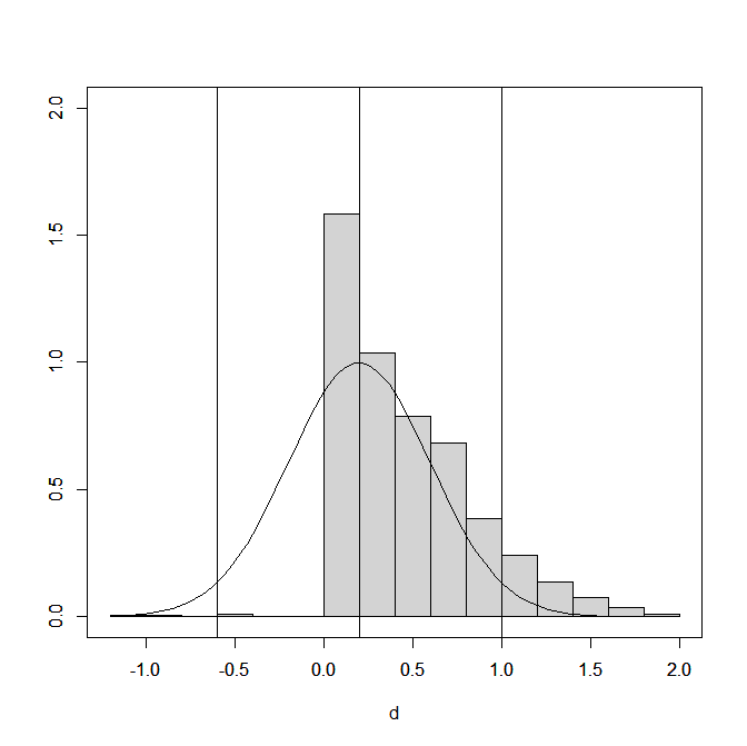
Figure 1 shows the distribution of the effect size estimates (extreme values below d = 1.2 and above d = 2 are excluded). The influence of p-hacking is visible

Histograms of effect sizes do not show the proportion of significant and non-significant results. This can be examined by computing the ratio of effect sizes over sampling error and treat these as approximate z-scores. Alternatively, the sample sizes can be used to compute t-values, and use the corresponding p-values to convert t-values into z-values.

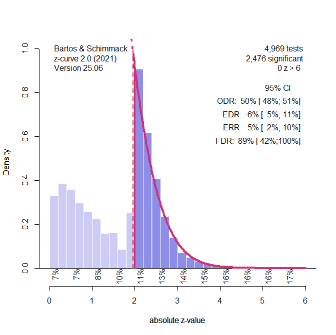
Figure 2 shows the plot of the z-values and the analysis of the z-values with z-curve, using the standard selection model that fits the model to all statistically significant z-values. The plot shows clear evidence of selection bias. Z-curve’s estimate of average power for the significant results is 5% (compared to the true value of 2.5% because the ERR takes the sign of replication results into account). The confidence interval includes the true value of 2.5%. Thus, the model does not reject the null hypothesis that all significant results are false positive results. The estimated average power for all positive results (i.e., the expected discovery rate, EDR) is estimated at 6%, while the true value is 5%. The 95%CI includes the true value. Incidentally, z–curve uses this result to estimate that 89% of the significant results are false positives, but the confidence interval includes the true value of 100%.

The simulation study shows the performance of z-curve with just 100 studies and a much smaller set of significant results that are used for model fitting. This will only widen the CI and is unlikely to change the result that z-curve performs well in this scenario.

Model Specifications

The specification of the z-curve model was explained and justified above.

Carter et al. (2019) observe conversion issues with the default (3PSM) selection model in some conditions. This is one of these conditions. However, the problem is that the 3PSM model assumes heterogeneity and has problems when all population effect sizes are the same. This does not mean that selection models cannot be used with those data. A solution is to test the random model and when it fails to run the fixed effects model. I used this approach and obtained usable results in all simulations.

The specification of the selection model remains the same as in the previous simulations and differed from Carter et al.’s default 3PSM model. First, I added steps to model different selection for positive and negative results. Second, I added a step to allow for different selection of non-significant and significant negative results. Third, I added a step to identify p-hacking that produces too many just significant results. The range of just significant results was defined as p-values between .05 and .01, two-sided. The one-sided p-value steps are c(.005,.025,.050,.500,.975).

P-uniform and PET-PEESE do not require thinking and were used as usual.

Selection Model (weightr)

The random-effects model failed to converge in 43% of the simulations. Actually, this is the better result because it implies zero heterogeneity, which is actually the true heterogeneity. In the other 57% of the cases, the random effects model estimated non-zero heterogeneity, average tau = ..01, average 95%CI = .00 to .08, 98% of confidence intervals included the true value of 0. Therefore, the selection model provides valuable information about heterogeneity and shows that there is very little or no heterogeneity. This is important because it implies that all sets of studies have the same average effect size and the estimate for all studies is the same as for sets selected for significance.

The fixed and the random effects model had difficulties estimating the selection weights for a model with several steps. However, the model with a single step that distinguishes significant positive and all other effect size estimates worked well. Therefore, I reran the simulation with a fixed effect model and a single step at p = .025 (one-tailed).

The average effect size estimate for all studies was d = -.03, average 95%CI = -.06 to .00, and 67% of the confidence intervals included the true value of zero. Moreover, the other confidence intervals implied a small negative effect. The reason is that p-hacking introduces a negative bias in selection models because p-hacking produces more just significant results than really significant results, but the selection model assumes that they are just as likely to be selected as really significant results when the null-hypothesis is true. However, the bias is really small. Thus, the selection model provides the correct information about the effect size for all studies and because it shows that there is no heterogeneity, the results also imply that even the subset of studies with positive and significant results contains only false positive results.

The selection model also detected bias, although it was not able to distinguish between selection and p-hacking. The average selection weight for non-significant results was d = .10, average 95% = .03 to .18, and none of the confidence intervals included a value of 1 that would indicate no bias.

To summarize, the main problem for the selection model was that the model had to be reduced to a two-component model (2PSM), without a random parameter for heterogeneity, tau fixed at 0, and a single step to distinguish significant and non-significant results. This model fit well and correctly revealed that the 100 studies lack evidential value.

PET-PEESE

PET regresses effect sizes on the corresponding sampling errors. The average estimate was d = -.05, 95%CI = .-.13 to .03, and 78% of the confidence intervals included the true value of zero. Thus, PET also shows a negative bias due to p-hacking, but the bias is also small.

PEESE regresses the effect sizes on the sampling variance (i.e., the squared sampling error). It is only relevant, if PET shows a positive and significant result. This was not the case in this simulation. PEESE results also show no effect, d = -03, 95%CI = -.07 to .02, and 83% of confidence intervals included the true value.

In short, PET-PEESE performs well in this simulation, but it does not perform better than the selection model. .

P-Uniform

P-uniform also has a bias test, but it detected bias in only 8% of the simulations. Thus, the selection model has a better bias test.

The average effect size estimate for the set of studies with positive and significant results was d = -.15. Thus, the model is more strongly biased than the other models. The reason is that it does not use the non-significant results and p-hacking has a stronger influence on the small subset of studies with significant results. The small sample size of significant results also implies that the confidence interval is very wide, average CI = -1.07 to .25. While 95% of confidence intervals included the true value of 0, 65% of confidence intervals also included a value of d = .2, which is considered a small effect size. Thus, the model makes it more difficult to rule out that a set of studies has evidential value. In short, p-uniform does not add useful information in this simulation.

Z-Curve

One way to test selection bias with z-curve is to fit the model to all positive results, non-significant and significant results, and to test for the presence of excessive just significant results (z = 2 to 2.6 ~ p = .05 to .01). This test was only significant in 67% of all simulations. Thus, the selection model has more power to detect bias.

Z-curve did show that the studies lacked evidential value. That is, confidence intervals always included power of 5%, but this information was also provided by the selection model.

Conclusion

The main conclusion from this specific simulation study is that it was necessary to specify a fixed-effect selection model with a single step. This model always converged, always showed evidence of bias, and slightly underestimated the true effect of zero. PET-PEESE performed as well. P-uniform and z-curve did not do well because they rely on significant results and on average only 30% of the results were significant, limiting the sample size to about 30 studies, while the other models could use all 100 studies.

The high percentage of non-significant results also has other implications. First, this simulation of p-hacking is mild. Stronger p-hacking would turn more non-significant results into significant results. The high percentage of non-significant results is also not representative of many research areas in psychology because success rates in psychology journals are 90% or higher. Z-curve and p-uniform were developed to deal with situations of strong bias.

Finally, the simulation of mild p-hacking and no selection bias implies that a meta-analysis that does not assume bias would also produce reasonable estimates. The weighted mean of the observed effect size estimates is d = .03. Thus, p-hacking has a weak influence on the results. A simple correction for bias is to use only the non-significant results. The estimated effect size is d = -.01. This correction has a negative bias because positive and significant estimates are excluded, but the effect is very small. The comparison of the two estimates shows that the true average is close to zero. Of course, using the selection model is better, but the point here is that the simulated condition is not particularly interesting. There was never a lot of bias to correct here. This is very different from real data, where naive meta-analyses show effect sizes of d = .6 and bias-corrected estimates range from 0 to .3 (Carter et al., 2019). Future studies need to examine more severe p-hacking scenarios.

In short, this condition is not particularly interesting, but it also does not pose a challenge for the selection model. Thus, the selection model remains the model to beat, and Simulation 100 (d = 0, tau = 0, & high selection bias) remains the most problematic scenario for the selection model.