You can find links to the other chapters on the post with Chapter 1.

Chapter 2 shows the use of z-curve.3.0 with the Open Science Collaboration Reproducibility Project (Science, 2015) p-values of the original studies.
zcurve3.0/Tutorial.R.Script.Chapter2.R at main · UlrichSchimmack/zcurve3.0

Introduction to Chapter 2

Z-curve was developed to examine the credibility (publication bias, replicability, false positive risk) of articles that report statistical results, typically null-hypothesis significance tests. The need for such a tool became apparent in the early 2010s, when concerns about replication failures and high false positive risks led to a crisis of confidence in published results.

Another remarkable investigation of the credibility of psychological science was the Reproducibility Project of the Open Science Collaboration (Science, 2015). Nearly 100 results published in in three influential journals were replicated as closely as possible. The key finding that has been cited in thousands of articles was that the percentage of significant results in the replication studies was much lower, and that effect sizes were much smaller as well.

In line with the emphasis on transparence, the project also made the data from this study openly available. The data provide a valuable learning tool to illustrate the use of z-curve.3.0. The data from this project are unique in that z-curve results based on the original results can be compared to the results of the replication studies. Normally, the “truth” is unknown or simulated with simulation studies. Here, the replication studies serve as an approximation of the truth. For example, the replicability estimate based on the p-values of the original studies can be compared to the actual outcome of the replication studies. Chapter 2 analyzes the original data. These analyses serve as a blueprint for typical applications of z-curve. Chapter 3 shows how z-curve analysis of replication studies can also provide useful information.

2.0 First Examination of the Z-curve Plot

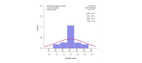
The first step is to run a quick z-curve analysis with the fast density function and no bootstrap and then change parameters to adjust the y-axis and the width of the histogram bars to make the figure visually appealing.

Visual inspection of the plot suggests that there is selection bias, as there are many more just significant results than non-significant results. By default, the model is fitted to the significant results only. The model then predicts the distribution of non-significant results. The actual data show 91% significant results. This is the observed discovery rate (ODR). The model estimates an expected discovery rate of only 41%. This also suggests publication bias, but point estimates are inconclusive.

Z-curve.3 provides a simple test of bias. This test assumes that there is no bias (the null-hypothesis). Under this assumption, z-curve is fitted to all z-values, not just significant ones. Bias will produce too many just significant results, like the bar with z-values between 2 and 2.4 in Figure 1. The default range for just significant results is 2 to 2.6 (about p = .05 to .01).

Figure 2 shows that z-values between 2 and 2.4 cannot be fitted by the model. The test of Excessive Just Significance (EJS) is significant with p = .0025. This confirms that bias is present in this dataset, but it does not tell us whether it is selection bias (not reporting non-significant results) or p-hacking (analyzing data in multiple ways until a significant result is found).

The next analysis examines p-hacking. P-hacking tends to produce more p-values that are just significant compared to actual power of studies. To test this, z-curve is fitted to the “really” significant results, z > 2.6, and the percentage of observed just significant results is compared to the prediction by the model.

Figure 3 shows the results. There are too many significant results between 2 and 2.4, but not between 2.4 and 2.6. The significance test is not significant, p = .1324. However, the selection model does not explain the excess of z-values between 2 and 2.4. We can now respecify the model and define “just significant” as 2 to 2.4.

Now the test is significant with p = .0009. But we tested twice. Did we just p-hack a p-hacking test? Not really. We can adjust alpha to take into account that we tested twice. Even with alpha = .025, the p-value of .0009 is significant.

The next test examined heterogeneity by comparing a model with a single component with a free mean and a fixed SD of 1 against (a) model with a single component free mean and free SD, and (b) a model with two components with free means and fixed SD of 1. Neither test showed evidence of heterogeneity.

Now we face a decision problem. Assuming no bias would lead to inflated estimates of power, but using a selection model when p-hacking was used leads to underestimation of power, especially, the estimate of power for all z-values, including non-significant ones. Both results should be reported, but I prefer to use the selection model and treat the downward bias due to p-hacking as a p-hacking penalty. Having access to the data and the z-curve program makes it possible for everybody to make their own decisions.

The final model is fitted with the “EM” algorithm and 500 bootstraps implemented in the z-curve.2.0 package. The EM algorithm is slower, but slightly superior to the density approach.

The final model confirms the presence of bias and quantifies it. The ODR is 91%, while the EDR is only 20%. Although the 95%CI is wide, it does not include the ODR. The Expected Replication Rate is 60%, with a 95%CI ranging from 44% to 74%. Chapter 3 will compare this to the actual results. Based on the EDR, it is possible to quantify the false positive risk; that is, the probability that a significant result was obtained without an effect (the null-hypothesis is true). The risk is 21%, but the 95%CI is wide and allows for 88% false positive results. This does not mean that many results are false positives, but it does mean that the evidence is weak and that many results could be false positives. Chapter 3 examines the false positive risk based on the actual replication results.

Although the heterogeneity test did not find evidence of heterogeneity, the local power results below the x-axis suggest that there is some heterogeneity. Non-significant results are estimated to have low power ranging from 20% to 32%. Significant results are estimated to have modest power for z-scores of 2 to 4. The value of 80% that is recommended for a priori power-analysis is only reached at z = 4 and very few studies have z-values greater 4. Thus, one clear finding is that the studies were underpowered. To avoid false negatives in replication studies, sample sizes would have to be increased considerably for most studies.