In this series of blog posts, I am reexamining Carter et al.’s (2019) simulation studies that tested various statistical tools to conduct meta-analysis. The reexamination has three purposes. First, it examines the performance of methods that can detect biases to do so. Second, I examine the ability of methods that estimate heterogeneity to provide good estimates of heterogeneity. Third, I examine the ability of different methods to estimate the average effect size for three different sets of effect sizes, namely (a) the effect size of all studies, including effects in the opposite direction than expected, (b) all positive effect sizes, and (c) all positive and significant effect sizes.

The reason to estimate effect sizes for different sets of studies is that meta-analyses can have different purposes. If all studies are direct replications of each other, we would not want to exclude studies that show negative effects. For example, we want to know that a drug has negative effects in a specific population. However, many meta-analyses in psychology rely on conceptual replications with different interventions and dependent variables. Moreover, many studies are selected to show significant results. In these meta-analyses, the purpose is to find subsets of studies that show the predicted effect with notable effect sizes. In this context, it is not relevant whether researchers tried many other manipulations that did not work. The aim is to find the one’s that did work and studies with significant results are the most likely ones to have real effects. Selection of significance, however, can lead to overestimation of effect sizes and underestimation of heterogeneity. Thus, methods that correct for bias are likely to outperform methods that do not in this setting.

I focus on the selection model implemented in the weightr package in R because it is the only tool that tests for the presence of bias and estimates heterogeneity. I examine the ability of these tests to detect bias when it is present and to provide good estimates of heterogeneity when heterogeneity is present. I also use the model result to compute estimates of the average effect size for all three sets of studies (all, only positive, only positive & significant).

The second method is PET-PEESE because it is widely used. PET-PEESE does not provide conclusive evidence of bias, but a positive relationship between effect sizes and sampling error suggests that bias is present. It does not provide an estimate of heterogeneity. It is also not clear which set of studies are the target of this method. Presumably, it is the average effect size of all studies, but if very few negative results are available, the estimate overestimates this average. I examine whether it produces a more reasonable estimate of the average of the positive results.

P-uniform is included because it is similar to the widely used p-curve method,but has an r-package and produces slightly superior estimates. I am using the LN1MINP method that is less prone to inflated estimates when heterogeneity is present. P-uniform assumes selection bias and does not test for it. It also does not test heterogeneity. Importantly, p-uniform uses only significant results and estimates the average effect size of the set of studies with positive and significant results. It does not provide estimates for the set of only positive results (including non-significant ones) or the set of all studies, including negative results.

Finally, I am using these simulations to examine the performance of z-curve.2.0. Using exactly the simulations that Carter et al. (2019) used prevents me from simulation hacking; that is, testing situations that show favorable results for my own method. I am testing the performance of z-curve to estimate average power of studies with positive and significant results and the average power of all positive studies. I then use these power estimates to estimate the average effect size for these two sets of studies. I also examine the presence of publication bias and p-hacking with z-curve.

Simulation 296

I focus on a sample size of k = 100 studies. Many meta-analyses have smaller sets of studies, but some do have 100 studies or more. Fewer studies will mainly lower the power to detect bias and produce wider confidence intervals in estimates.

The first simulation examines how the methods perform when no biases are present. For bias tests, this condition examines the false positive risk. With alpha = .05 or 95%confidence intervals, bias should be detected in no more than 5 out of 100 simulations.

The key parameters of this simulation are an average effect size of d = .2 and large heterogeneity, tau = .4. This simulation assumes that 95% of effect sizes are in the range from -.6 to 1 and that most effect sizes are small. The percentage of results with a negative sign in this simulation is a bit implausible, but it helps to see the differences between the three sets of studies.

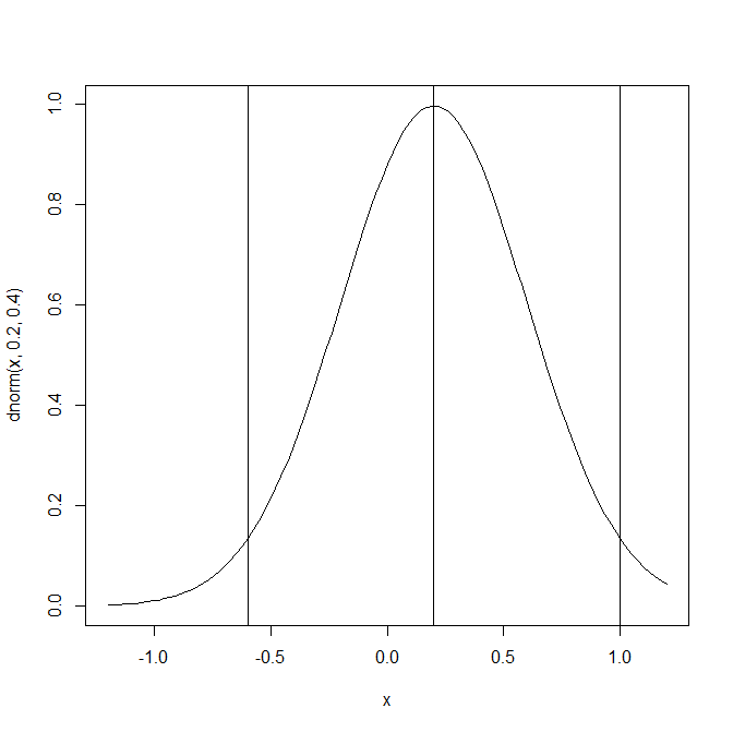
The average effect size for all studies is of course d = .2. Selecting only positive results produces an average effect size of d = .38. The set of positive results with significant results depends on the sample sizes of the studies. Sample sizes in the Carter et al. (2017) simulation varied widely from N = 10 to N = 3124 with a mean of N = 134 and a median of N = 52. Running a large simulation produced a rate of 9% significant results with a negative sign and 24% significant results with a positive sign. The power of producing a significant result for only the positive results was 38%. The average effect size for studies with positive and significant results was d = .57. Thus, this simulation implies that expected significant results are obtained with strong effect sizes that are stronger than most actual effect sizes in psychology.

Selection Model (weightr)

Carter et al. (2019) observe conversion issues with the selection model in some conditions. In this simulation, no problems were encountered. The estimated effect size for all studies was d = .19, average 95%CI .04 to .35. 93% of the CI included the true value of .20. I consider this an acceptable performance. The estimated heterogeneity was close to the true value, tau = .39, average 95%CI = .28 to ..47, but coverage was a bit lower than the 95%CI suggests, 88%. Based on these mean and tau estimates, I computed an effect size estimate for the positive results of d = .37, average 95%CI = .18 to .53, 96% coverage. This is also a good performance. The estimated mean for the positive and significant results was d = .57, average 95%CI = .36 to .73 with 96% coverage.

Selection for significance would produce too few non-significant results. This is tested with the selection weight for p-values between .025 (one-sided) and 1. A value of 1 implies no selection bias. The average estimate was 1.16, average 95%CI = .04 to 2.28. 87% of confidence intervals included the true value. The other 13% showed false evidence of selection bias.

To test for p-hacking, I specified a model with a step at p = .005 (one-sided). The model then computes a weight for the proportion of p-values in the range between .025 (one-sided) and .005 (one-sided) that corresponds to two-sided p-values between .01 and .05. P-hacking would produce too many significant results in this range. The weight for p-values between .01 and .05 (two-sided) was 1.19, average 95%CI = .08 to 2.30. 91% of CIs included a value of 1, indicating no evidence of p-hacking. The other CIs produced values less than 1. Thus, none of the confidence intervals suggested p-hacking.

In sum, the selection model performed flawlessly in this condition.

PET-PEESE

PET regresses effect sizes on the sampling error. The average estimate was close to the average for all studies, d = .19, 95%CI = .05 to .33. However, only 62% of confidence intervals included the true value. When PET produces a positive and significant result, it is recommended to run a second regression with the variance (sampling error squared) as predictor. This is called the PEESE model. In the absence of any bias, the results are practically the same.

In this specific condition, the selection model is clearly preferable to the PET-PEESE approach. First, it produces more accurate estimates of the average effect size (better coverage of the confidence interval). Second, it produces an estimate of heterogeneity that can be used to compute averages for subsets of studies with positive results or positive and significant results. Third, it tests for the presence of bias and can provide evidence that bias is not present or small. In this case, it is also possible to run normal meta-analytic models, but the results would be no different from the selection model. The only reason to use PET-PEESE would be that the model performs better in other situations, when the selection model fails (Carter et al., 2019).

P-Uniform

The p-uniform estimate is d = .42, 95%CI = .31 to .50. It is often stated that p-uniform overestimates effect sizes in the presence of heterogeneity. However, this claim is based on the comparison of p-uniform estimates to the true average for all studies, d = .2. This is not a plausible comparison because p-uniform estimates are based on the subset of significant results and the method estimates the average effect size of this subset. This average is always going to be higher than the overall average when heterogeneity is present. What is more disturbing is that the p-uniform method is not even able to estimate the average effect size of the positive and significant results correctly. Compared to the true average of d = .57, the estimate is too low and only 25% of the confidence intervals include the true value. P-uniform also does not provide information about the presence of bias or estimate heterogeneity. In short, the method fails in this specific condition.

Z-Curve

The estimated average power of positive and significant results was 66%, 95%CI = 58% to 73%. All confidence intervals included the true value. This overperformance is explained by the conservative confidence intervals implemented in z-curve. The average power before selection for significance was estimated to be 40%, 95%CI = 31% to 48%. The coverage was 100%. Based on the average power of studies selected for significance, z-curve estimated an average effect size of d = .56, 95%CI = .46 to .68. The 95%CI included the true parameter 92% of the time. This is clearly better than p-uniform, but not better than the selection model that also provides information about heterogeneity in effect sizes. The estimate for the average effect size for all positive results (based on the estimated power before selection for significance) was d = .40; 95%CI = .31 to .50 with 91% coverage. This is not a bad performance, but the selection model did better.

To test for bias, the model compared the observed percentage of z-values between 2.0 and 2.4 with the predicted percentage of just significant results in this range. The average observed percentage was 23.4%. The average predicted percentage was 23.0%. Only 3% of the significance tests showed false evidence of bias with alpha = .05. Thus, the test has the intended error rate.

Conclusion

Based on this single condition from Carter et al.’s (2019) meta-analysis, the selection model is clearly superior to all other models. It provides information about the presence of bias and heterogeneity and it provides good estimates and confidence intervals for the estimates of the overall average and heterogeneity. These values can be used to get good estimates of the average effect size for subsets of studies with only positive results or only positive and significant results.

The information about heterogeneity is particularly important. An estimate of tau = .4 shows large heterogeneity. It is implausible that such big differences could be observed in a meta-analysis of direct replication studies. Evidence of such large heterogeneity should trigger a careful examination of the data to see whether coding mistakes or other errors produced unexpected heterogeneity.

Large heterogeneity, however, is to be expected in psychological meta-analysis that combine apples, oranges, grapes, and other fruits in one salad. In these ‘fruit-salad’ meta-analyses, the overall effect size is meaningless and easily misinterpreted. For example, with a median effect size of N = 52 and an average effect size of d = .2, a study has virtually no power to detect an effect. This might lead to the conclusion that the entire literature is underpowered. However, an analysis of the subset of studies with positive and significant results shows an effect size of d = .57 that can be detected even with small samples of N = 52. A focus on the subset of studies with positive and significant results would produce a tasty salad of studies that can be replicated. This was the idea behind p-curve, but p-curve and p-uniform are not the best tools to look for tasty fruit. As noted by McShane et al., selection models can do a better job.

If you found this post interesting, you probably want to know how the selection model (and other models) perform when selection bias and p-hacking produce too many significant results. Well, stay tuned for the next post that examines p-hacking.